The Reproduction Ability of a Numerical Model for Simulating the Outflow Rate of Backfilling Materials from a Coastal Structure

Abstract

In very shallow areas, the frequency by which coastal structures (like dikes and seawalls) are directly broken by large wave forces is low because large waves are broken in deeper areas. The main cause for such destruction is ground scour in front of the structures and outflow of backfilling materials by middle-scale waves; therefore, the scour and the outflow should be considered when designing a coastal structure in a very shallow area. In this paper, a numerical model consisting of CADMAS-SURF, which can calculate fluid motion in porous media, and empirical equations for simulating the outflow phenomena are introduced; thereafter, practical calculations on field cases in Thailand and Japan are demonstrated. Additionally, since the effects of wave periods and water depth to the outflow rate have never been clarified, hydraulic model experiments, empirical calculations using an existing formula, and numerical simulations are performed in order to examine these effects on the outflow rate. The simulated results using the numerical model align well with the experimental results. Moreover, both results show that the outflow rate is proportional to the wave period and inversely proportional to water depth.

1. Introduction

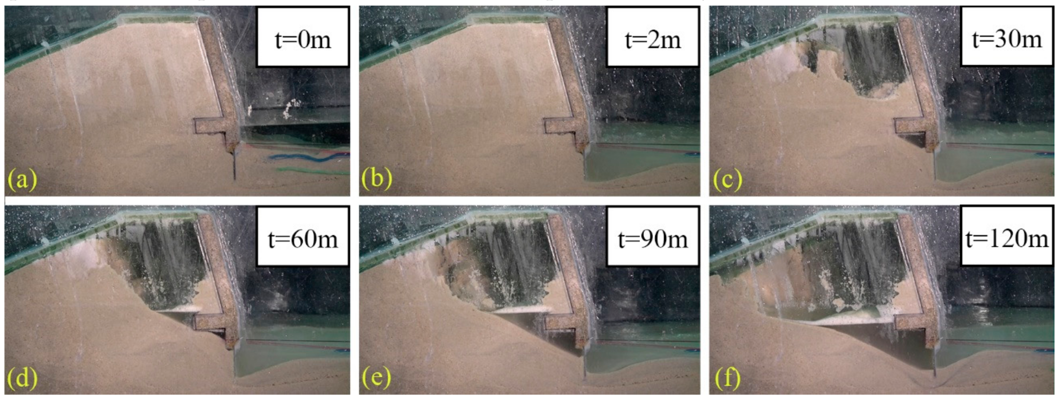
Many coastal dikes and seawalls constructed in very shallow areas in our surveys were seen to be damaged or destroyed by waves smaller than the designed waves. This resulted from scour in front of the structures and the outflow of backfilling materials from their bodies. Scour is the process by which bed materials around coastal structures are removed by hydrodynamic forces, which diminish the soil stability in front of the structures and can cause damage or failure to the structures, e.g., a slide of the armor surface or a complete overturn. To visualize outflow, an example hydraulic model experiment is introduced. In this experiment, a 1/30 dike model filled with sand (median grain size = 0.2 mm) was continuously hit by irregular waves, during which the significant wave height was 0.223 m, and the significant wave period was 2.65 s. This experiment uses a dike in the Hirono Coast in Shizuoka Prefecture, Japan and the wave conditions of Typhoon No. 9 from 1997 (H_1/3 = 6.69 m, T_1/3 = 14.5 s) as a prototype. The direction of the outflow is the offshore direction. When the effects of wave diffraction or shaded areas are not considered (e.g., the effects of detached breakwaters or breakwaters), the mechanism of outflow phenomena can be analyzed in two dimensions. Since the generated waves were uniform in the alongshore direction, the alongshore transportation in the experiment can be neglected. The experimental result is shown in Figure 1. In a coastal dike or a seawall filled by granular materials (e.g., Figure 1a), when the scour depth in front of the structure reaches the lowest edge of the structure (e.g., a sheet pile) (Figure 1b), incident waves can penetrate under the body of the structure. Thereafter, when the shear resistance at the lowest edge of the structure becomes smaller than the shear force generated by the return flow, the backfilling materials flow out via the return flow through the edge of the structure. When the materials at the lowest edges flow out, the remaining materials are moved to fill the void by the gravity until the slope becomes stable. In this way, the formation of a cave occurs (Figure 1c–f). This motion of backfilling materials is called the outflow (or suction). When the structure loses its backfilling materials, the stability and the protective ability of the structure become weaker than their designated values. Then, when middle-scale waves hit the structure, the possibility that the structure will be destroyed is high.

There are many methods for evaluating scour depth in front of coastal structures induced by waves. Fowler [1], for example, proposed an empirical equation to evaluate the maximum scour depth in front of a vertical seawall induced by irregular waves by using midscale experiments. Another method uses a numerical model to simulate scour; for example, the model of Ca et al. [2] can reproduce scour depths on various coasts with acceptable accuracy.

However, there are few predictive methods for the outflow rate. For empirical methods to determine the outflow rate, Yamamoto and Minami [3] studied the mechanism of outflow phenomena by using experiments with a wave flume and a dike model. They were able to reproduce the outflow from a concrete-covered dike in Hirono Coast, Japan, which was damaged by Typhoon No. 9 in 1997. After they confirmed the reliability of their experimental methodology, they used their method to examine the effects of various parameters on the outflow rate. The results show that shear resistance decreases when the sand layer thickness in front of the structure becomes thinner and the outflow rate increases when the median grain size becomes finer. Due to these results, the authors proposed an empirical method for predicting the failure of a dike or a seawall induced by outflow. Ioroi and Yamamoto [4] performed many experiments in order to determine the relationship between the outflow rate and the pore water pressure, the return flow velocity, and the median grain size of backfilling materials. They proposed an empirical outflow formula that could consider the effects of the median grain size, the sand layer thickness at the front of the structure, the maximum pore water pressure, and the maximum return flow velocity. Kuisorn et al. [5] performed field surveys on many coasts in Thailand and reported outflow damage on these coasts. They calculated the outflow rates by using Ioroi and Yamamoto’s formula; the results show that the formula could be applied to field cases with acceptable accuracy.

Maeno et al. [6] and Kotani et al. [7] reported that the cyclic action of water pressure on the sand layer precipitated the formation of a cave inside a structure and caused the failure of the structure. The authors proposed a numerical model for simulating cyclic water pressure, based on the poro-elastic theory, which could simulate the cyclic pressure under a simple seawall. Nakamura et al. [8] proposed a simulation model based on the Volume of Fluid technique and the Biot model. Their model could simulate the outflow rate from the lowest edge of a rubble revetment. These models are limited by the shapes of structures. Following this, Silarom et al. [9] proposed a numerical model consisting of CADMAS-SURF (Super Roller Flume Computer-Aided Design of Maritime Structure) and empirical equations for calculating the time change of the outflow rates from coastal dikes and seawalls with arbitrary shapes.

In this paper, the authors reproduced the outflow phenomenon in field cases—the coasts of Oarai–Isohama, Ishikawa–Komatsu in Japan, and Suan Son in Thailand—by using Silarom et al.’s model in order to confirm the reliability of the model and examine the outflow damage of each coast. The effects of wave heights, median grain sizes, uniformity, and dry density have been studied by Ioroi et al. [10]. However, the effects of water depth and wave periods on the outflow rate are still unclear. Since wave periods and water depth influence wave breaking criteria, which affect sediment transportation in the adjacent area of the structures, and pore water pressure inside the structures attenuates when water depth becomes deeper, the effects of these parameters must be clarified. Thus, some experiments were performed in order to examine the effects of these parameters on the outflow. In the present examinations, a hydraulic model, the numerical model of Silarom et al. [9], and the empirical formula of Ioroi et al. [10] were used.

2. The Concept of the Model

2.1. The Sediment Transport Model

The outflow of backfilling materials can be understood as a sheet flow of a layer of materials. It is believed that bedload particles are moved by the shear force acting on the surface layer of the bed, and this movement is resisted by the shear strength of the bed. Typically, a formula, Equation (1), for calculating the bedload transport rate, has a form proportional to the 1.5th power of the difference between the shear force and the critical shear force according to the assumption that this rate is proportional to the power generated by the shear force:

$$\frac{q}{w_s{D}_{50}}=m{(\left|\theta \right|-{\theta }_c)}^{1.5}\frac{\theta }{\left|\theta \right|},$$

(1)

where q is the bedload transport rate (volume) per unit width; w_s is the settling velocity of the bed particle; D₅₀ is the median grain size of the bed materials; m is the proportional coefficient (unitless); θ is the Shields parameter (dimensionless shear stress); and θ_c is the critical Shields parameter (dimensionless critical shear strength).

However, when the region of the outflow is the inner side of a structure, which is semi-enclosed or enclosed by the structure, the movement of the sediment is mainly controlled by excess pore water pressure (=”the total pore water pressure” - “the static pore water pressure”). Thus, the outflow rate should be considered as a function of this pressure. The critical shear strength on the outflow layer can be calculated by using the Coulomb–Terzaghi shear strength equation, shown in Equation (2), and the shear force acting on the outflow layer can be calculated by using the fluid force equation shown in Equation (3). Since the outflow occurs when a soil layer in front of the structure is entirely scoured, the critical shear strength in front of the structure must be a function of the excess pore water pressure. Moreover, since the fluid pressure is proportional to the square of the flow velocity, the shear stress must be a function of this pressure as well. Therefore, the outflow rate should be proportional to the difference between the Shields parameter (dimensionless shear stress) and the critical Shields parameter (dimensionless critical shear strength), which can be calculated using Equations (4) and (5), respectively, by considering that the rate is a function of the excess pore water pressure. In summary, when the inflow rate is very small compared to the outflow rate, the flow velocity of Equation (3) can be specified as the return flow velocity, and thus the outflow rate formula can be expressed as shown in Equation (6). For the proportional coefficient, β, Silarom et al. [9] proposed an empirical equation, Equation (7), to calculate the coefficient by using experiments and simulation tests.

$${\tau }_r=(({\rho }_s-{\rho }_w)g{d}_t-p)\tan \varphi ,$$

(2)

$${\tau }_f=\frac{f}{2}{\rho }_{{}_w}{u}^2,$$

(3)

$$\theta =\frac{{\tau }_f}{({\rho }_s-{\rho }_w)g{D}_{50}},$$

(4)

$${\theta }_c=\frac{{\tau }_r}{({\rho }_s-{\rho }_w)g{D}_{50}},$$

(5)

$$\frac{q}{w_s{D}_{50}}=\beta (\theta -{\theta }_c),$$

(6)

$$\beta =0.321\exp \left(-0.25\left(\frac{D_{50}}{0.2}\right)\right),$$

(7)

where τ_r is the critical outflow force (the shear resistance due to the critical shear strength on the outflow layer to the return flow); ρ_s is the density of the backfilling materials; ρ_w is the density of water; g is the gravitational acceleration; d_t is the layer thickness of the backfilling materials; p is the excess pore water pressure; ϕ is the internal friction angle of the backfilling materials; θ_c is the dimensionless critical outflow force; τ_f is the outflow force (the shear stress due to the return flow); f is the outflow force coefficient (=1); u is the flow velocity; θ is the dimensionless outflow force; β is the proportional coefficient; q is the outflow rate (including porosity); and the unit of D₅₀ in Equation (7) is “mm”.

2.2. CADMAS-SURF

CADMAS-SURF [11] is a numerical wave flume for maritime structural design, which was developed by the Coastal Development Institute of Technology, Japan. This model can simulate wave dynamics, wave-structure interactions, and, especially, fluid motion in a porous medium, which can be used for outflow calculation. In the 2D version, hydrodynamics is simulated mainly by the continuity equation, Navier–Stokes motion equations, and the Volume of Fluid technique. The flow in a porous medium that can be treated by using two methods—one is the drag force coefficient method, and the other is the Dupuit–Forchheimer (D–F) method. The D–F method can adequately consider the effects of pressure attenuation due to either precast concrete armor units (e.g., hollow tetrahedrons, tetrapods, and hexapods), spherical or cubic concrete blocks, stones, or pebbles.

By using this model, the time history of the pressure and velocity inside the backfilling materials of a structure can be calculated and then used for the outflow rate calculation; however, the calculated pressure distribution inside a covered coastal dike (the front slope and a crown part are covered by concrete, and a leeward slope is covered by asphalt or concrete) and a covered seawall (the front slope and the crown part are covered by concrete) filled by very fine materials seems to be overestimated because this model cannot sufficiently consider the effects of fine grains (D₅₀ < 1 mm) [9,10]. The reasons for this limitation are as follows:

1) Since the suitable value for the drag force coefficient for very fine materials is very large, and this value is a value depending on the Reynolds number, it is difficult to use the drag force coefficient method.

2) The Dupuit–Forchheimer method was derived from a steady flow stage and empirical coefficients are required for each material. Although there are recommended values of these coefficients for precast concrete blocks, stones, and pebbles, which can be used with reasonable accuracy, there is no such a value for very fine materials. Moreover, the smaller value of the median grain size affects the stability of the calculation; thus, it is difficult to use this method for various cases with different material characteristics, especially in coastal areas, which consist of fine sand.

To handle this problem, Silarom et al. [9] studied the pore water pressure distribution inside a dike model and the changing of the pore water pressure for the dimensions of a cave by using pore pressure meters installed in the dike. The positions of the pore pressure meters include a dimensionless inner horizontal length (the inner horizontal length/the horizontal length at the lowest edge of the dike) of 0, 0.067, 0.2, and 0.677. Then, the authors proposed empirical equations for obtaining reduction coefficients to improve the pressure calculated by CADMAS-SURF. These empirical equations are as follows:

1) The empirical equation, Equation (8), for determining the reduction coefficient of the inner length inside a structure: the experimental results show that the (dimensionless) pore water pressure decreases when the inner length inside the dike increases, and the layer thickness becomes thinner. This empirical equation was obtained by using the best matching function for the diagram of the experimental results when there is no thinned layer. Thus, the equation can be used to improve the horizontal pressure distribution inside the structure.

$$C_x={0.00022}^{x/x_{\max }},$$

(8)

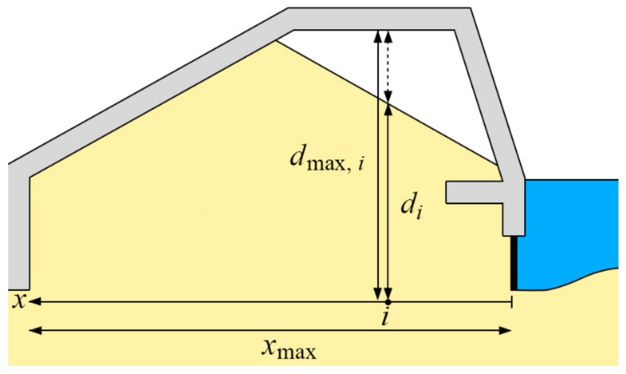
where C_x is the reduction coefficient for the inner length inside the structure; x is the inner horizontal length at the lowest edge from the front of the structure (refer to Figure 2); and x_max is the total horizontal length at the lowest edge of the structure.

2) The empirical equation, Equation (9), for obtaining a reduction coefficient by the backfilling layer becoming thin: since Equation (8) can consider pressure attenuation only when there is no cavity inside the structure, this empirical equation is proposed to consider cases where the pressure decreases when the backfilling layer is thinned by the outflow. The experimental results show that pressure attenuation due to the formation of a cave is not only a function of the thickness of the backfilling materials but also a function of the inner length inside the dike. Thus, by analyzing a diagram of the pressure changes due to the thinned heights at some inner lengths inside the dike, Equations (9) and (10) were obtained.

$$C_d=\left\{\begin{array}{ll}\exp \left(0.269-\frac{0.263}{d/d_{\max }}+\chi \ln (d/d_{\max })\right)& \mathrm{when} C_d\le 1\\ 1\hfill & \mathrm{when} C_d>1\end{array}\right.,$$

(9)

$$\chi =45.0-23.7\exp \left(\frac{-(x/x_{\max })-3.265}{4.953}\right),$$

(10)

where C_d is a reduction coefficient by the backfilling layer becoming thin; d is the thickness of the backfilling layer at the inner length of x; and d_max is the maximum thickness of the backfilling layer at the inner length of x.

3) The empirical equation, Equation (11), for obtaining a coefficient for the median grain size: the experimental results show that the pore water pressure decreases when the median grain size of the backfilling materials becomes larger. Since the actual size of the median diameter of the very fine backfilling materials cannot be set in CADMAS-SURF due to the reasons mentioned above, this equation was proposed to improve the calculated pressure. Some trial simulations were performed and compared to the experimental results in order to find the suitable value of this coefficient for various diameters (0.2, 0.66, and 5 mm). By using the relation between this coefficient and the median grain size, Equation (11) was obtained.

$$C_{D_{50}}=0.65{\left(\frac{0.2}{D_{50}}\right)}^{0.85}+0.35,$$

(11)

where the unit of D₅₀ is “mm”.

By using these empirical equations, the effect of pore water pressure attenuation due to fine backfilling materials and the formation of a cave can be considered, as expressed in Equation (12).

$$p_{\mathrm{MOD}}=C_x{C}_d{C}_{D_{50}}\left(p_{\mathrm{CAD}}-{\rho }_{w}gh\right),$$

(12)

where p_MOD is the modified pressure; p_CAD is the pressure calculated by CADMAS-SURF; and h is the local static water depth.

2.3. The Simulation Procedure

By using CADMAS-SURF and the empirical equations, the outflow rate and the outflow volume (the time integral of the outflow rate) can be calculated using the outflow force and the critical outflow force calculated from the modified pressure and calculated velocity in each time step. The following steps outline the procedure of the simulation:

1) Set the dimension of the obstacles (impermeable structures), porous media, and wave conditions in CADMAS-SURF.

2) Determine the measuring line at the lowest edge of the structure. This line should be around 1 to 3 meshes below the lowest edge of the structure. The vertical length from this line to the elevation of the backfilling surface in each mesh is defined as d_max,i for the initial time and d_i for the other, where i is the mesh number in the horizontal direction. This line is also used as the datum line to calculate the static water pressure in Equation (12).

3) Calculate the proportional coefficient, β, using Equation (7).

4) Calculate the reduction coefficients, C_x, C_d, and C_D50, using Equations (8)–(11).

5) Calculate the pressure and velocity in each mesh on the measuring line using CADMAS-SURF, then modify the calculated pressure using Equation (12).

6) If the direction of the flow velocity is out of the structure, calculate the outflow resistance and the outflow force on each mesh using Equations (13) and (14). Then calculate the Shields parameter, the critical Shield parameter, and the outflow rate using Equations (4)–(6).

$${\tau }_r=(({\rho }_s-{\rho }_w)gd-p_{\mathrm{MOD}})\tan \varphi ,$$

(13)

$${\tau }_f=\frac{f}{2}\rho U_{{}_{\mathrm{CAD}}}^2,$$

(14)

where U_CAD is the calculated return flow velocity in the horizontal direction from CADMAS-SURF.

7) Calculate the thinned height of the backfilling materials in each mesh by using the continuity equation for sediment transport, Equation (15).

$$\frac{\mathsf{\Delta }{q}_i}{\mathsf{\Delta }x}=\frac{\mathsf{\Delta }{d}_i}{\mathsf{\Delta }t},$$

(15)

where Δt is the time step, and Δd_i is the thinned height of the backfilling materials.

8) Subtract the backfilling layer thickness by the thinned height, calculated using Equation (16), in each mesh.

$$d_i^{t+\mathsf{\Delta }t}=d_i^t-\mathsf{\Delta }{d}_i^t.$$

(16)

9) Check the slope stability by using the assumption that the slope of the backfilling materials must not exceed the repose angle of the materials. This argument is shown in Equation (17). If the calculated slope does not agree with Equation (17), the thickness of the calculated mesh and the next mesh are adjusted until they satisfy the argument.

$$\frac{d_{i+1}^t-d_i^t}{\mathsf{\Delta }x}\le \tan {\theta }_{\mathrm{repose}},$$

(17)

where θ_repose is the angle of repose (≈30° for wet sand).

10) Compute the next time step.

3. Outflow Rate Simulation in Field Cases

Practical simulations were performed to validate the reliability of the model and examine outflow damage of the target coasts. The outflow damage on the coasts of Oarai–Isohama and Ishikawa–Komatsu in Japan, and Suan Son in Thailand was reproduced. The simulation conditions, including the structural dimensions, initial backfilling materials volumes, median grain size, and wave conditions for each case are shown in

Table 1. Wave conditions and structural information in the simulations.

Names of Coasts	Significant Wave Height, H1/3 (m)	Significant Wave Period, T1/3 (s)	Front Bottom Depth, ht (m)	Tidal Level (m)	Median Grain Size, D50 (mm)	Initial Backfilling Materials Volume (m3/m)	Measured Outflow Volume, Qm (m3/m)	Calculated Outflow Volume, Qc (m3/m)	Percentage Error (%)
Oarai–Isohama	5.1	10.8	–3.5	0.45	0.2	145	20	10.1	49.5
Ishikawa–Komatsu	6.0	10.5	–2.5	0.58	0.6	71.2	16	12.0	25.2
Suan Son	3.0	6.0	–0.3	-	0.2	7.8	3.0	3.77	25.7
Hirono	4.45	13.9	0	0.70	0.4	74.2	28	31.5 *	12.5
Khlong Wan	3.5	6.2	0.1	1.30	2.0	4.5	3.5	2.20 *	37.4
South Patong	3.0	7.2	0.8	0.80	1.0	5.4	3.2	2.54 *	20.6

*: The calculated outflow volumes were extracted from the report of Silarom et al. [9].

(the wave conditions of the Hirono Coast extracted from Silarom et al. [9] are the wave conditions of Typhoon No. 18 from 1997). The duration times of these simulations were set to 6 h, according to the report of Yamamoto and Minami [3], who mentioned that the duration of strong wind by a typical typhoon is about 10 h, which can be separated into 4 h of scour and 6 h of outflow. Detailed information on each case is given below.

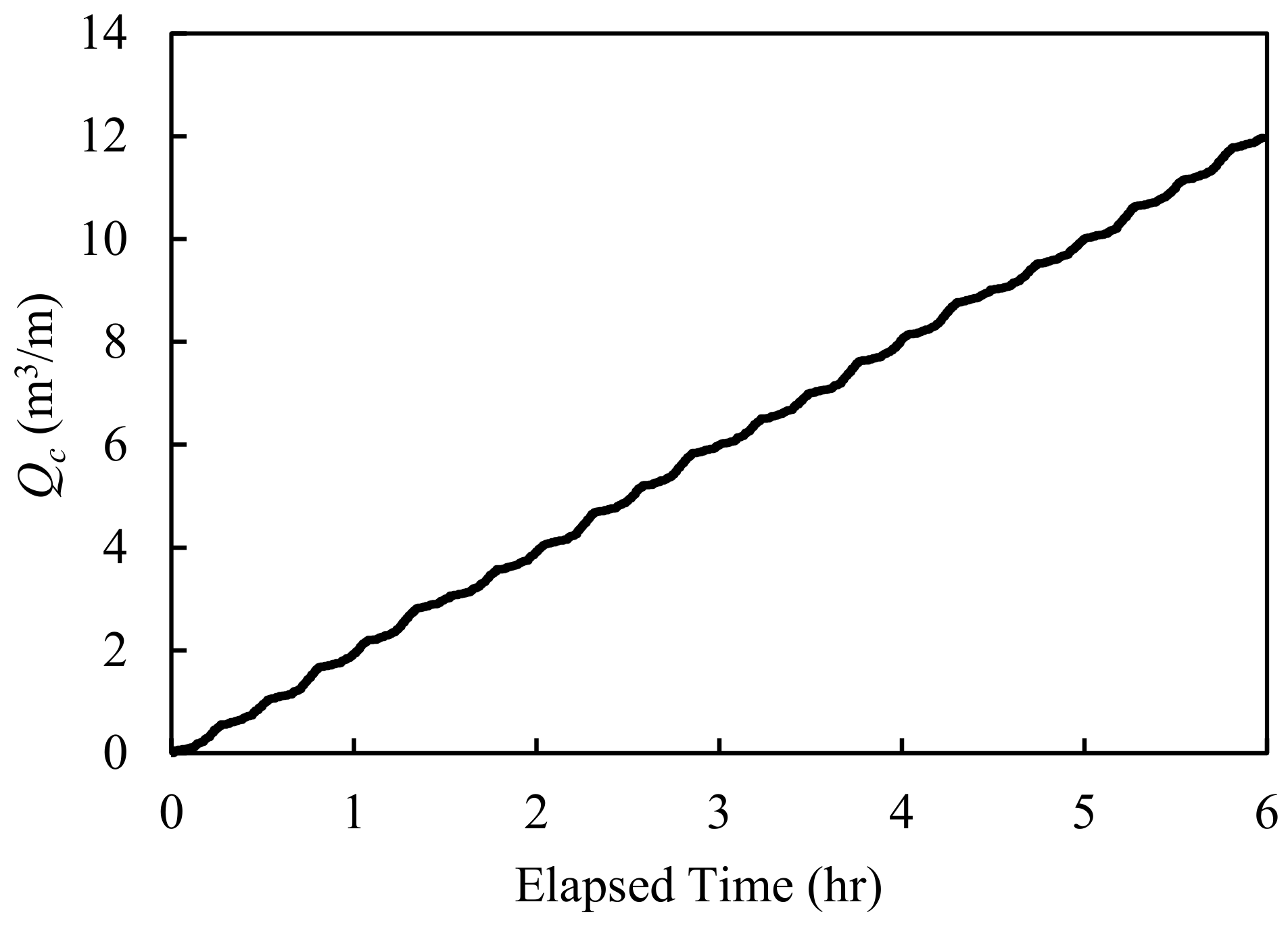
3.1. Oarai–Isohama Coast

The study case is a seawall constructed in an extended sandy beach in front of Oarai Aquarium located on the Oarai–Isohama coast in Ibaraki Prefecture, Japan (the Pacific Ocean side). This beach has suffered heavy erosion since it was constructed in the 1960s. The seawall has been gradually exposed to waves, and a cavity inside the seawall has formed since October of 2015. In order to calculate the outflow rate, the dimension of the seawall and the wave characteristic of Typhoon No. 23 in 2015 were extracted from the report of Uda et al. 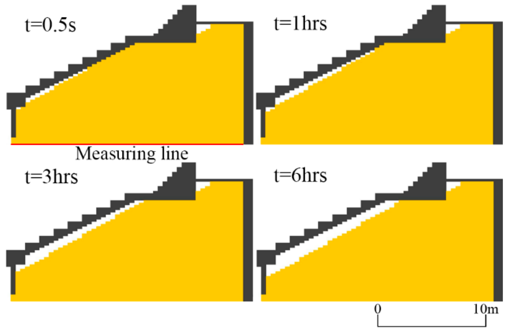[12], as shown in Table 1. The maximum outflow volume per unit width was estimated from the field survey’s photographs. 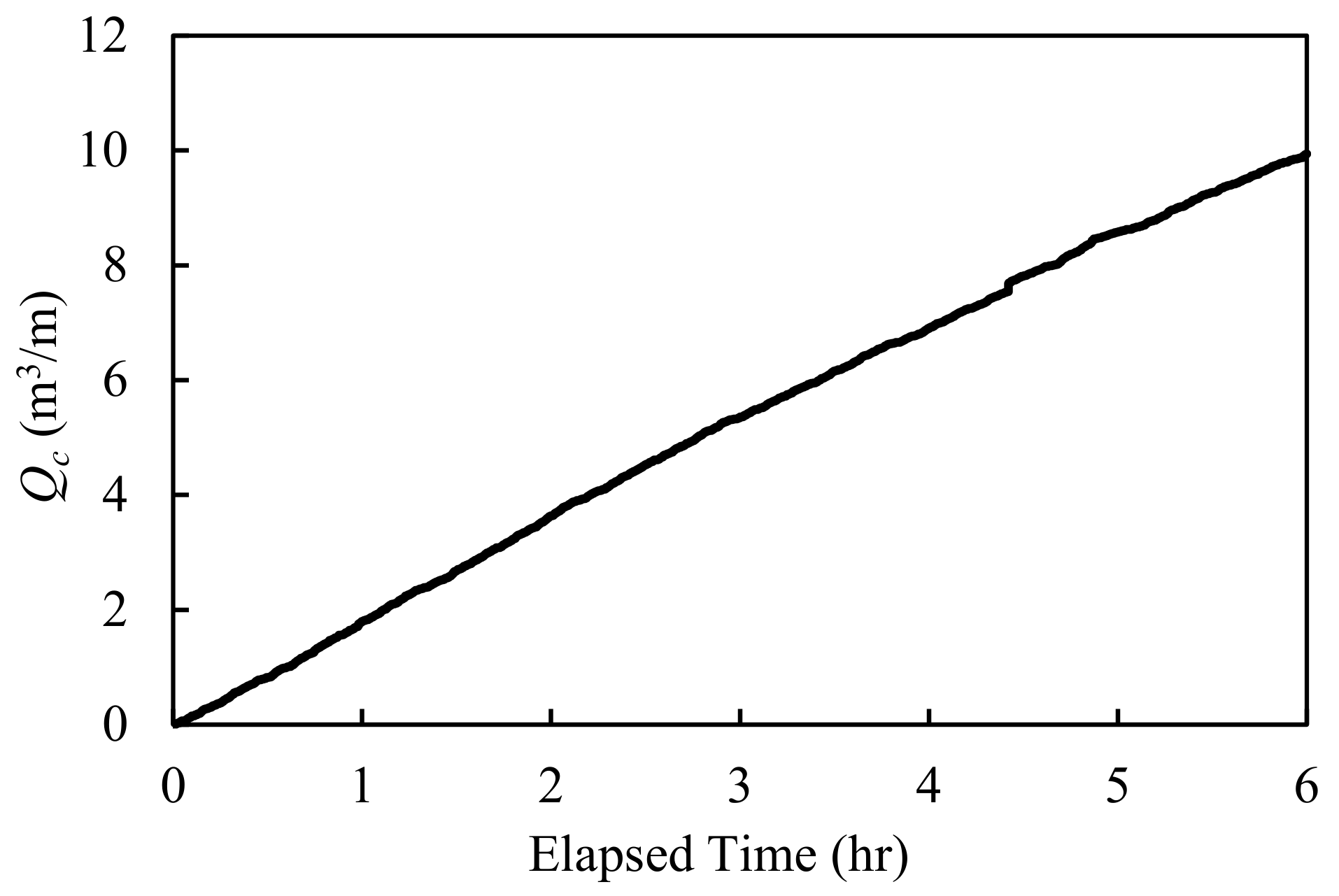The simulated results are shown in Figure 3 and Figure 4.

The results show that the outflow rates were a constant value, regardless of the simulation time. This is because the total amount of the outflow volume was small compared to its size. According to Equations (9) and (10), the reduction coefficient, C_d, depends on changing the layer thickness of the backfilling materials. At the front of the structure, where x/x_max = 0, the coefficient is a constant value of 1 when the parameter d/d_max is greater than 0.14. Therefore, since changes in the thickness were small, the coefficient became a constant value, resulting in constant outflow rates.

The calculated volume is underestimated compared to the measured volume because the model cannot consider cracks on the structure. The percentage error is 49.5%. In the field, incident waves infiltrated into the body of the structure through these cracks, resulting in the additional leakage of backfilling materials. The measured outflow volume is small compared to the size of the seawall. Even though the calculated volume is underestimated, since the both of measured and calculated outflow volumes are small compared to the size of the seawall, the results are practical when using the calculated result to examine the degree of damage induced by the outflow. The calculated cave shows that there is no supporting material below the front slope of the seawall. Thus, the calculated results show that the stability of the structure must be weaker than its design value.

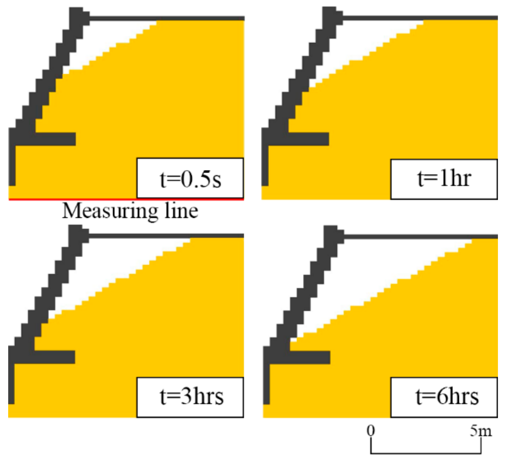
3.2. Ishikawa–Komatsu Coast

This coast is located in Komatsu city, Ishikawa Prefecture, Japan (the Japan Sea side). According to the heavy erosion in the area, the local government decided to construct a concrete dike and detached breakwaters in order to prevent coastal hazards on the seaside. However, the concrete dike was damaged by Typhoon No. 15 in 2001, during which a cavity was found in the body. The dimension of the dike and the wave conditions were extracted from the report of Yamamoto and Minami [3] in order to simulate the outflow. The simulated results are shown in Figure 5 and Figure 6.

The calculated outflow rate was also a constant value for the same reason as the Oarai–Isohama Coast. The calculated result was underestimated because the model cannot consider the effects of cracks. Like the Oarai–Isohama Coast, the calculated outflow rates were large enough to remove the support materials from the front slope of the dike, which has a significant effect on the stability of the dike.

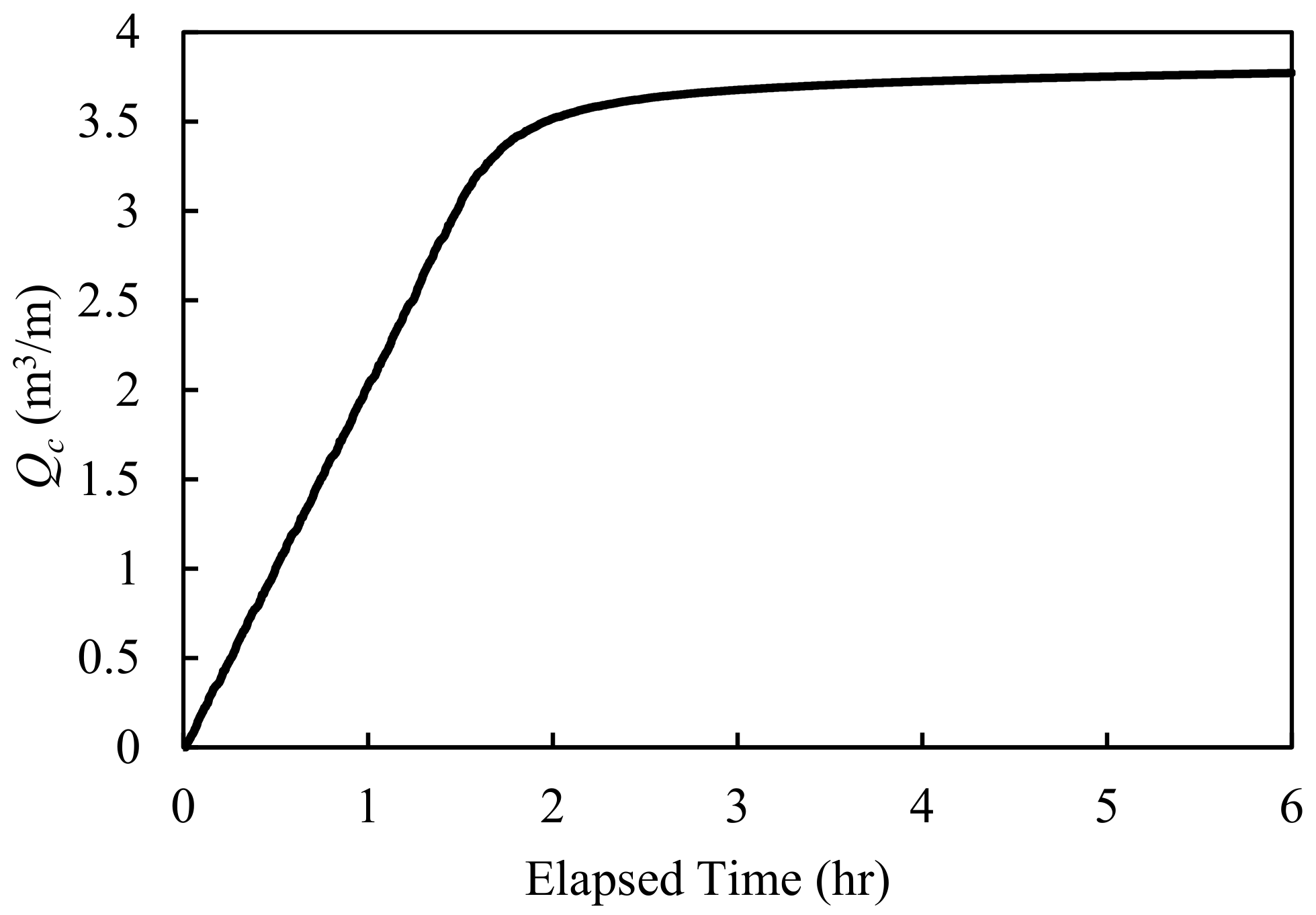
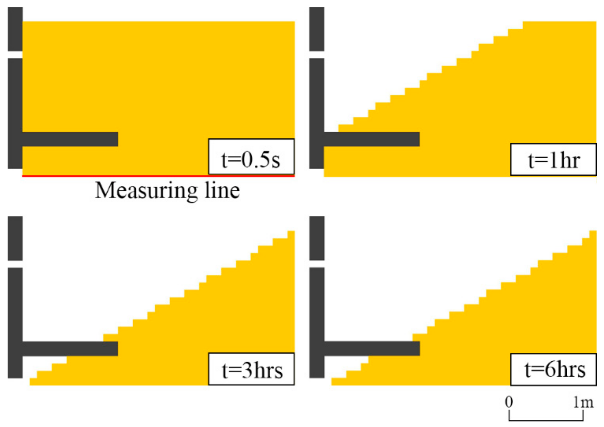
3.3. Suan Son Coast

The Suan Son Coast is located in Rayong Province, on the eastern portion of the Gulf of Thailand. This coast is a famous beach for tourists and a recreational area for local people due to its wide sandy beach and mild slope. A vertical seawall was constructed by the local government to protect the seaside road and the coastal area of the province. Based on the field surveys of Kuisorn et al. [5], the seawall was damaged by leakage of the backfilling materials induced by wave overtopping and the outflow. The outflow rates were simulated by using the crown height, bottom depth, and wave conditions extracted from their survey report. The simulated results are shown in Figure 7 and Figure 8.

The time series of the outflow volume shows that there are two stages of the outflow rate. The first stage is the constant stage, which occurred from the starting time to the elapsed time of about 1.5 h. At this stage, the outflow rates were constant (the same as those of previous coasts discussed above). During the second stage the outflow volume entered equilibrium, which occurred after an elapsed time of about 1.5 h. The outflow rates of this stage were significantly lower than those of the constant stage. The reason for using two stages was that the calculated outflow volume (≈3.7 m³/m) was large compared to the total amount of the backfilling materials (≈7 m³/m); thus, coefficient C_d in front of the seawall could be changed during the simulation when the parameter d/d_max was smaller than 0.14. This change resulted in a transformation of the outflow rate to the elapsed time. The calculated results show that a huge amount of the backfilling materials was removed; thus, the seawall is easily destroyed by middle-class waves (wave height = 2–3 m).

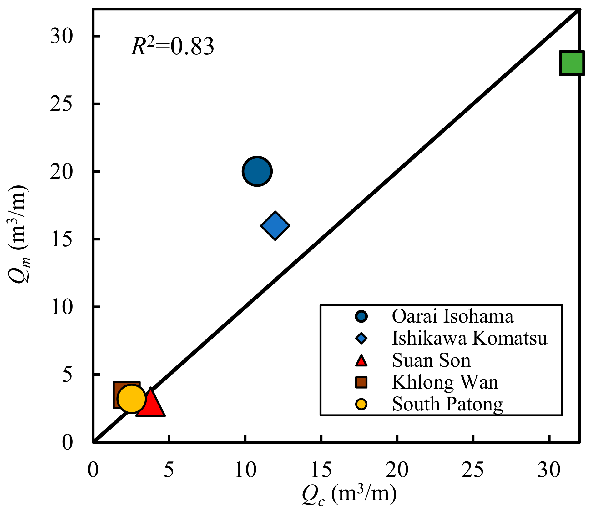
A comparison between the measured outflow volumes and calculated outflow volumes of all cases is shown in Figure 9. Moreover, in order to improve the reliability of the correlation coefficient, the simulated results from the report of Silarom et al. [9], as shown in Table 1, were added to the correlation graph. The accuracy of the calculated results on the Oarai–Isohama Coast is not good. However, the outflow volume of this coast is small when comparing the measured and the initial amount of the backfilling materials. Thus, whether using the calculated results or measured results, the degree of damage is not significantly different. The accuracies on the other coasts seem to be acceptable. Therefore, even though the accuracy is not perfect, since the correlation coefficient is good (R² = 0.83), this model can be used to examine the degree of damage induced by the outflow.

4. Examination of the Effects of Water Depth and Wave Periods on the Outflow

The effects of many parameters on the outflow rate have been elucidated by some researchers. For example, Ioroi and Yamamoto [4] and Ioroi et al. [10] performed many experiments and proposed an empirical outflow formula that can consider the effects of pore water pressure, return flow velocity, median grain size, the dry density, and the uniformity coefficient. However, there is no available information on the effects of water depth and wave periods. Since the wave period and water depth influence the flow velocity, the wave steepness, Iribarren number, and so on (which in turn affect the coastal sediment processes, and thus the outflow rate), it is important to examine these parameters to elucidate their effects on the outflow rate. In this section, the authors performed hydraulic model experiments to determine the relation between these parameters and the outflow. Moreover, the authors conducted examinations to check whether the empirical formula of Ioroi et al. or the numerical model of Silarom et al. can consider the effects of wave periods or water depth.

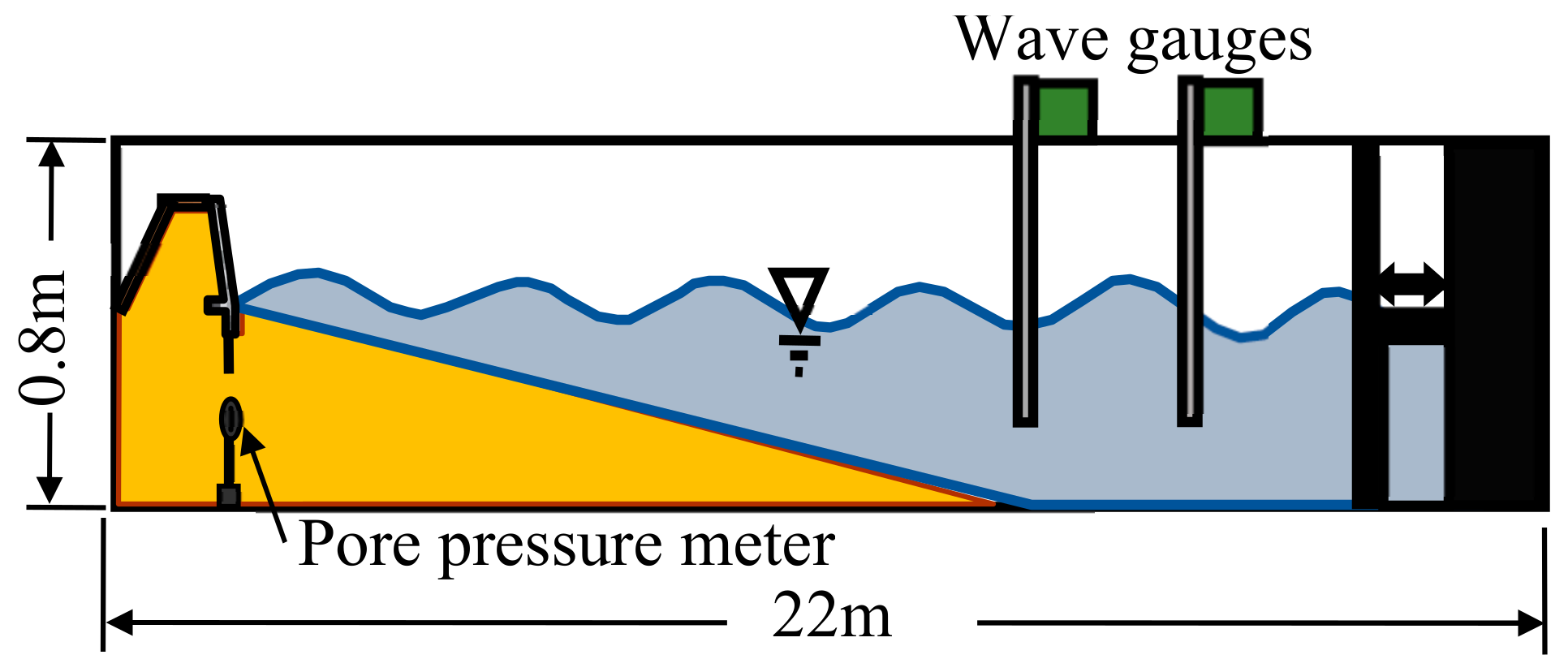
A dike model with a scale of 1/30 was set in a wave flume, with a width of 0.5 m, a height of 0.8 m, and a length of 22 m, as shown in Figure 10. The seaward slope of the dike was made of concrete, the crown part and the leeward slope were made of acrylic plates, and all joints were sealed with silicone. The dike model represents a typical dike in Japan in which the face is made of concrete, and the crown part and leeward slope are made of concrete or asphalt. The initial backfilling materials was about 0.12 m³/m. According to the stable beach slope formula of Yamamoto et al. [13], the stable beach slope for the experiments is from 1/30 to 1/16. However, in order to reproduce the heavy scour and outflow rate, the front beach slope of 1/15 was used. This slope is the average slope for eroded beaches in Japan. Irregular waves were generated by a ball-screw-driven wave generator and measured with wave gauges. The Bret–Schneider wave spectrum was used. The wave reflection was controlled by software of wave generator. Some testing experiments were performed in order to verify the accuracy of the input signals for the wave generator. A pore pressure meter was set under the sheet pile of the dike. The geometry, significant wave height, and significant wave periods were scaled using Froude’s law of similitude. For the median grain size, Ito and Tsuchiya [14] studied the grain size ratio of the model as a prototype by using small- and large-scale model experiments and proposed a diagram for obtaining the grain size ratio. By using this diagram, an accurate scale of the grain size can be obtained. Thus, the median grain size of the backfilling materials was scaled by using the similarities of the beach profiles by Ito and Tsuchiya. This methodology can be used to reproduce outflow phenomena on the Hirono Coast as shown in Figure 1. The significant wave height and median grain size of the backfilling materials were set to 0.12 m and 0.2 mm, respectively. The experimental conditions and external forces used in the experiments are shown in

Table 2. Experimental conditions and external forces.

Case	Significant Wave Height, H1/3 (m)	Significant Wave Period, T1/3 (s)	Wave Steepness in Deep Water	Water Depth, h0 (m)	Water Depth at the Toe of the Dike, ht (m)	Measured Outflow Volume Qm (m3/m)
E-1	0.12	2.00	0.0192	0.35	0.05	0.052
E-2	0.12	2.00	0.0192	0.40	0.10	0.038
E-3	0.12	2.00	0.0192	0.50	0.20	0.005
E-4	0.12	1.50	0.0342	0.50	0.20	0.003
E-5	0.12	2.50	0.0123	0.50	0.20	0.018

.

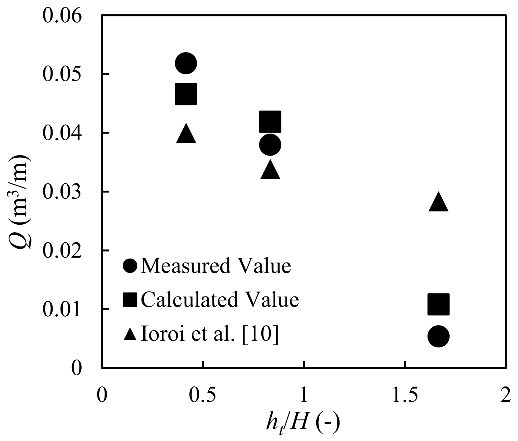
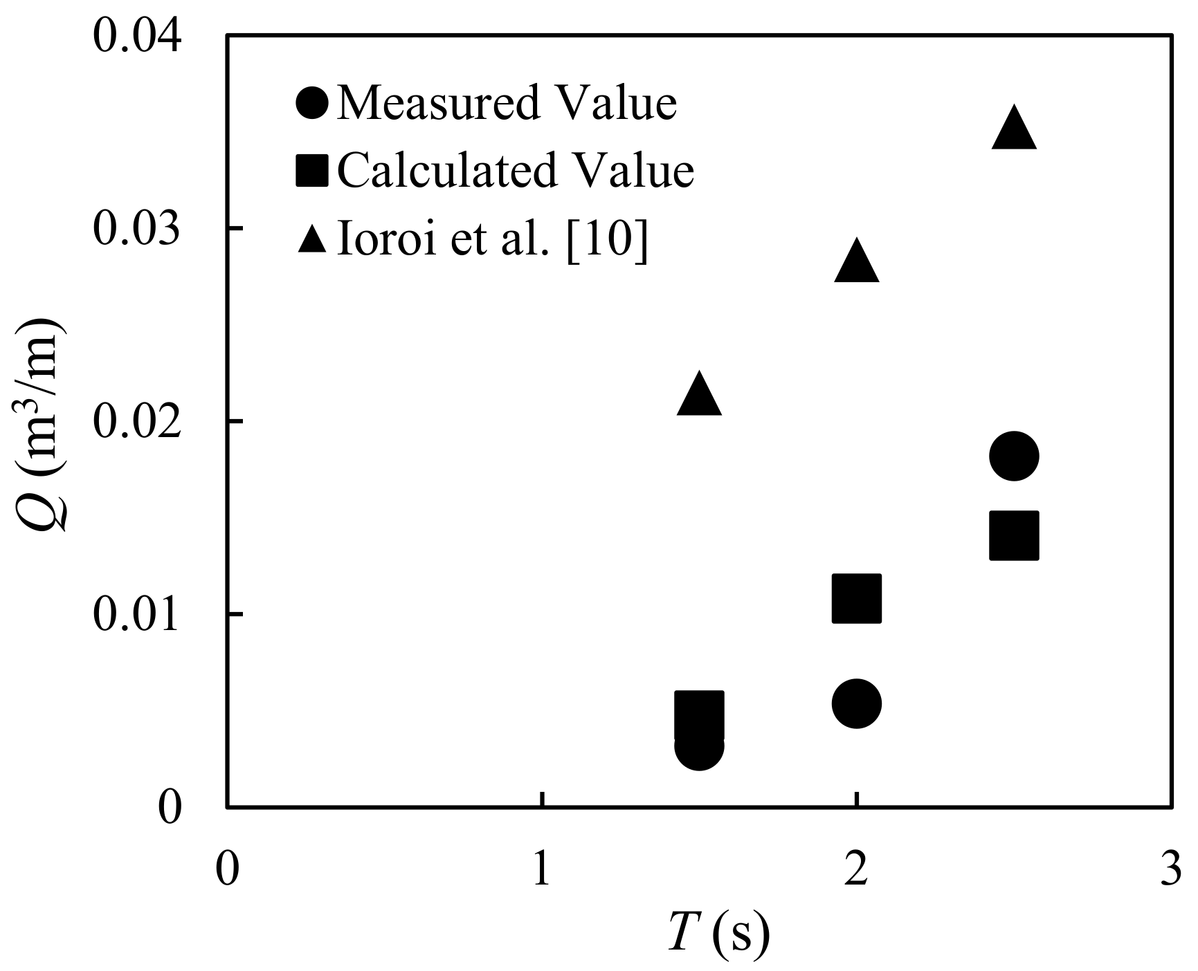
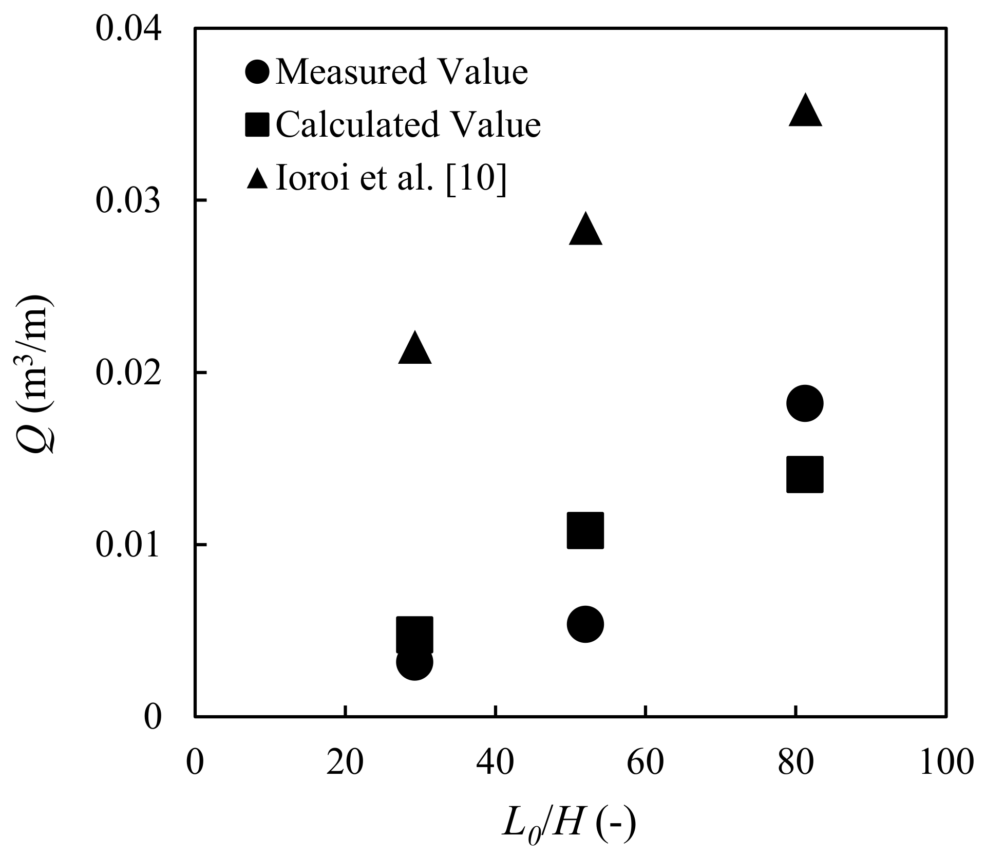
The experimental results are shown in Figure 11 and Figure 12. The results indicate that the outflow volume increases when the wave period increases and decreases when the water depth increases. These trends are similar to those of the maximum scour depth in front of a seawall (e.g., in [15,16]). By considering the wave periods in terms of wavelengths in deep water, the results shown in Figure 13 were obtained. The results show that the outflow rate is proportional to the wavelength in deep water, which is a function of T² (L₀ = gT²/2π).

To confirm that the same trends can be calculated by using the numerical model consisting of CADMAS-SURF and the empirical equations, simulations on the same wave conditions were implemented. The wave conditions in the front of the dike are the same as those of the experimental ones. However, water depth in the offing area was increased by 25 cm because the wave-generation method cannot work when the water depth is insufficient. When the conditions in the adjacent area of the dike (e.g., the front beach slope and the water depth at the front of the dike) and the wave conditions in the offing area are the same, the wave breaking point and the wave breaking criteria must be the same, and thus, the incident wave conditions in front of the dike must be the same. Therefore, this technique can be used. The simulation conditions are shown in

Table 3. Simulation conditions and external forces.

Case	Significant Wave Height, H1/3 (m)	Significant Wave Period, T1/3 (s)	Wave Steepness in Deep Water	Water Depth, h0 (m)	Water Depth at the Toe of the Dike, ht (m)	Calculated Outflow Volume Qc (m3/m)	Percentage Error (%)
S-1	0.12	2.00	0.0192	0.60	0.05	0.047	10.12
S-2	0.12	2.00	0.0192	0.66	0.10	0.042	10.30
S-3	0.12	2.00	0.0192	0.75	0.20	0.011	101.61
S-4	0.12	1.50	0.0342	0.75	0.20	0.005	49.80
S-5	0.12	2.50	0.0123	0.75	0.20	0.014	22.71

, and the calculated results are shown in Figure 11 Figure 12 Figure 13 Figure 14. A comparison between the results from the experiments and the simulations shows the same trend for the outflow volume. Even the absolute errors of cases S-3 and S-4 were not significantly different from those of other cases, but the relative errors of these cases were not good. It must be mentioned that the accuracy of the model is not good when the total outflow volume is very small. However, the results could show that the accuracy of the simulated relationship between the concerned parameters and the outflow rates is better than that of the existing empirical formula. When the outflow damage is a ratio between the total outflow volume and the initial backfilling materials, the significance of the difference between the measured outflow volume (E-3 and E-4) and the calculated outflow volume (S-3 and S-4) is small because these values were very small compared to the initial backfilling materials. Therefore, the results can be useful to evaluate the effects of the parameters or even a degree of damage.

Ioroi et al.’s formula, Equations (18)–(26), introduced empirical equations, Equations (23)–(26), for calculating the maximum pore water pressure and the maximum return flow velocity, which can be used to calculate the shear force and the shear resistance at the lowest edge of a dike by using Equations (21) and (22). These shears are used to calculate the outflow rate subject to the time rearrangement part (=0.5(1 + cos(αt/T))) of Equation (18), which can take the incident wave period into account. In this particular section, the validity of the wave period and the maximum elapsed time depends on the rearrangement coefficient, α, which can be expressed as t/T≤α/π. The time rearrangement coefficient depends on the median grain size. Thus, the validity of the maximum elapsed time is limited by the wave period and the median grain size. In other words, the accumulated sand outflow rate is directly affected by the wave during the maximum duration of the outflow. Moreover, since the wave period affects the shoaling coefficient, which affects the incident wave height, this formula can indirectly account for the effect of the wave period by considering the incident wave height in Equation (23) to be affected by the wave period. This formula can also consider the effects of water depth on the maximum return flow velocity by using Equation (26). When the water becomes deeper, the incident wave height becomes larger, and the pressure at the toe of a structure becomes smaller. However, the empirical equation for calculating the maximum pore water pressure, Equation (23), cannot consider the pressure attenuation due to water depth. Thus, the calculated maximum pore water pressure must be overestimated when applying this formula in deeper areas.

The examination of the formula was implemented using the maximum elapsed time for the imposed incident wave periods when the median grain size equals 0.2 mm, and the offing wave height was set to a constant value of 0.12 m. The parameters used in this examination are shown in

Table 4. Conditions used in the examination of Ioroi et al.’s formula.

Case	Significant Wave Height, H1/3 (m)	Significant Wave Period, T1/3 (s)	Wave Steepness in Deep Wate.	Water Depth, h0 (m)	Water Depth at the Toe of the Dike, ht (m)	Calculated Outflow Volume Qc (m3/m)	Percentage Error (%)
I-1	0.12	2.00	0.0192	-	0.05	0.040	22.74
I-2	0.12	2.00	0.0192	-	0.10	0.034	10.84
I-3	0.12	2.00	0.0192	-	0.20	0.028	429.70
I-4	0.12	1.50	0.0342	-	0.20	0.021	577.98
I-5	0.12	2.50	0.0123	-	0.20	0.035	94.01

. The calculated results are shown in Figure 11, Figure 12 and Figure 13.

The trends of the outflow volume are the same as those of the hydraulic model and the numerical model; thus, the outflow volume increases when the wave period increases. One reason is that the maximum elapsed time is proportional to the wave period. Thus, even this parameter cannot affect the shear force, the shear resistance, or the maximum outflow rate; when the elapsed time becomes longer, the accumulated outflow rate must become bigger. Another reason is that in the surf zone, the incident wave height becomes higher when the wave period becomes longer (refer to Goda’s estimation of wave height in the surf zone diagrams [17]). Thus, the outflow force becomes larger. However, the accuracy is not good when water depth becomes deeper. For the effect of water depth, this parameter affects the maximum return flow velocity, as expressed in Equation (26). However, this formula cannot consider pressure attenuation due to an increase in water depth. Thus, the calculated maximum pore water pressure and the calculated outflow rate must be overestimated when the water becomes deeper. Moreover, since this formula cannot consider the effects of wave breaking types, which have strong effects on the sediment transport in very shallow areas, but the wave period and water depth influence the wave breaking criteria, the accuracy of the formula is lower than expected. The reason that the accuracy of the numerical model is higher than that of the empirical formula is because CADMAS-SURF can simulate wave dynamics with higher accuracy, especially wave breaking and wave motion in front of a structure. Thus, the calculated pressure and velocity must be more accurate than those of the empirical formula, which considers the maximum pressure and the maximum velocity calculated by the empirical equations.

$$\frac{q}{w{D}_{50}}=\beta (\theta -{\theta }_c)\frac{1}{2}\left(1+\cos \left(\frac{\alpha t}{T}\right)\right),$$

(18)

$$\left.\begin{array}{cc}\alpha =-9.0\times {10}^{-5}(D_{50}/0.2)+0.0031\hfill & \hfill [1\le D_{50}/0.2\le 25]\\ \alpha =-3.39\times {10}^{-5}(D_{50}/0.2)+0.0017\hfill & \hfill [25\le D_{50}/0.2\le 50]\end{array}\right\},$$

(19)

$$\beta =0.028\exp \left(-0.35\left(\frac{D_{50}}{0.2}\right)\right) ,$$

(20)

$${\tau }_r=(({\rho }_s-{\rho }_w)g{d}_t-P_{ob\max })\tan \varphi ,$$

(21)

$${\tau }_f=\frac{f}{2}{\rho }_w{V}_{\max }^2,$$

(22)

$$\frac{P_{ob\max }}{{\rho }_{w}gH}=a\tanh {\left(\frac{0.03H}{d_t}\right)}^b,$$

(23)

$$a=0.37{(0.2/D_{50})}^{0.85}+0.30,$$

(24)

$$b=0.55{(0.2/D_{50})}^{0.78}+0.05,$$

(25)

$$V_{\max }=\sqrt{\frac{2P_{ob\max }}{{\rho }_w{\left(\frac{h_t}{H}+1.0\right)}^{1.11}}},$$

(26)

where α is the time rearrangement coefficient; P_obmax is the maximum pore water pressure during the return flows; V_max is the maximum return flow velocity; a and b are the coefficients calculated by Equations (24) and (25); h_t is the water depth at the toe of the dike; H is the incident wave height; and the unit of D₅₀ in Equations (19), (20), (24), and (25) is “mm”.

5. Conclusions

The examinations on the outflow damage on the coasts of Oarai–Isohama, Ishikawa–Komatsu, and Suan Son were implemented by using a numerical model consisting of CADMAS-SURF and empirical equations. The wave conditions, median grain sizes, and structural dimensions used in the simulations were extracted from the reports of Yamamoto and Minami [3] and Kuisorn et al. [5], as shown in Table 1.

The simulated results of the Oarai–Isohama Coast show that the total outflow volume is about 10 m³/m. The calculated formation of the cave inside the seawall shows that there is a cavity between the front slope and the backfilling materials, which has a strong effect on the stability of the seawall. The simulated results of the Ishikawa–Komatsu Coast indicate that the total outflow volume is about 12 m³/m. The formation of the cave shows that the supporting materials for the front slope and the crown part flowed out. Thus, the stability of the dike must be very low. The simulated outflow volume on the Suan Son Coast is about 3.7 m³/m. This amount is very large for its size, as there are no supporting materials for the wall. Thus, the seawall can be easily destroyed by middle-scale waves.

The reliability of the model is confirmed by comparing these simulated results to the measured values from the same reports. A correlation graph consisting of the simulated results of the authors and Silarom et al. [9] was created, as shown in Figure 9. This graph shows that the present model could calculate the outflow rates with acceptable accuracy (R² = 0.83). The simulated results for the Oarai–Isohama Coast and Ishikawa–Komatsu Coast were underestimated because the effect of cracks on these structures were not considered.

Moreover, the authors proposed the effects of water depth and wave periods on the outflow volume by using hydraulic model experiments. These experiments were performed by varying the water depth in front of the dike and the wave periods, as shown in Table 2. The results show that the outflow volume increases when the wave period increases and decreases when the water depth increases. It can be concluded that the outflow must be proportional to the wavelength and inversely proportional to the water depth.

The simulations using the simulation model and the calculations using Ioroi et al.’s formula (with the same conditions as the experiments, as shown in Table 3; Table 4) were carried out to ensure the reliability of the numerical model and the formula for these effects; the simulated results align well with the experimental results. Even though the accuracies when the total outflow volume is very small were not good, this model can be used to evaluate the relationship between concerned parameters and the outflow. For Ioroi et al.’s formula, the results show the same trend, but the accuracy when the water becomes deeper or when the wave period becomes longer is not good. The reason for this result is that Ioroi et al.’s formula cannot sufficiently account for the effects of these parameters on the pore water pressure and return flow velocity.

In the future, larger-scale experiments for cases E-3 and E-4 should be implemented to improve the accuracy of the model. In addition, more experiments using other parameters and conditions such as the uniformity coefficient, dry density, and cracked concrete (or a structure that has voids) should be performed to improve the consideration ability of the model. Lastly, more simulations in field cases with variable conditions (e.g., wave conditions and different shapes of the structures) need to be done to statistically improve the accuracy of the correlation coefficient of the model.