Assessment of Sea Level Rise at West Coast of Portugal Mainland and Its Projection for the 21st Century

Abstract

Based on the updated relative sea level rise rates, 21st-century projections are made for the west coast of Portugal Mainland. The mean sea level from Cascais tide gauge and North Atlantic satellite altimetry data have been analyzed. Through bootstrapping linear regression and polynomial adjustments, mean sea level time series were used to calculate different empirical projections for sea level rise, by estimating the initial velocity and its corresponding acceleration. The results are consistent with an accelerated sea level rise, showing evidence of a faster rise than previous century estimates. Based on different numerical methods of second order polynomial fitting, it is possible to build a set of projection models of relative sea level rise. Applying the same methods to regional sea level anomaly from satellite altimetry, additional projections are also built with good consistency. Both data sets, tide gauge and satellite altimetry data, enabled the development of an ensemble of projection models. The relative sea level rise projections are crucial for national coastal planning and management since extreme sea level scenarios can potentially cause erosion and flooding. Based on absolute vertical velocities obtained by integrating global sea level models, neo-tectonic studies, and permanent Global Positioning System (GPS) station time series, it is possible to transform relative into absolute sea level rise scenarios, and vice-versa, allowing the generation of absolute sea level rise projection curves and its comparison with already established global projections. The sea level rise observed at the Cascais tide gauge has always shown a significant correlation with global sea level rise observations, evidencing relatively low rates of vertical land velocity and residual synoptic regional dynamic effects. An ensemble of sea level projection models for the 21st century is proposed with its corresponding probability density function, both for relative and absolute sea level rise for the west coast of Portugal Mainland. A mean sea level rise of 1.14 m was obtained for the epoch of 2100, with a likely range of 95% of probability between 0.39 m and 1.89 m.

1. Introduction

After almost two decades of continuous observations of the digital acoustic Cascais tide gauge (TG), operated under the responsibility of the actual national authority, the Directorate-General for Territorial Development (DGT), it is now possible to estimate sea level rise rates with lower uncertainties and increased reliability. From November 2003 to present, the acoustic TG has recorded sea level, initially with a rate of 6 min, and since 2010 with an updated rate of 3 min. A daily mean sea level data set, created from the combination of these data and data acquired, from 2000 to 2003, by the previous analogical TG installed at Cascais (Figure 1), has been used to monitor mean sea level interannual variations, due to storm surge, other oceanic and atmospheric forcing factors, and mainly due to sea level rise (SLR) caused by regional eustatic changes. To guaranty the reliability of the results, spirit-leveling observations relative to a reference benchmark and to the Cascais EUREF (Regional Reference Frame Sub-Commission for Europe) permanent GNSS (Global Navigation Satellite Systems) station of Cascais (CASC) have been periodically performed (annually or once in two years) for monitoring vertical displacements of the TG site and respective benchmark.

The effects of climate change due to global warming are mostly recognized as the main driving force for global SLR [1]. The eustatic component of SLR is driven mainly by two forcing factors, the thermal expansion, due to the increase of ocean heat content (nowadays measured mainly by the ARGO float network, http://www.argo.net), and the ocean mass change, due to the melting of glacier and ice sheets and the discharge of land water reservoirs. Data collected by the GRACE (Gravity Recovery and Climate Experiment) mission satellites and by the ARGO float network, from 2005 onwards, have been used to quantify and validate these two forcing factors of eustatic SLR, showing a strong agreement with Topex/Poseidon and Jansen I & II satellite altimetry data series [2].

The variation of relative mean sea level (MSL) depends, mainly, on the eustatic variation of the global mean sea level (GMSL), on regional ocean dynamic effects (such as heat flux and wind-driven currents), and on regional vertical movements of the crust (tectonic and post-glacial isostatic adjustment). To transform relative into absolute SLR, or to adjust tide gauge rates to regional satellite altimetry data rates, the absolute vertical land velocity must be evaluated, usually, from reliable GNSS time series from a nearby permanent station combined with precise spirit-leveling data. However, through the direct comparison of relative MSL time series obtained from TG data with data resulting from satellite altimetry and secular GMSL series, or alternatively, from available neo-tectonics studies, one might also obtain vertical velocity estimations. Since for the Cascais TG, all these types of data are available, so the results can be easily compared to convert relative to absolute SLR.

While relative SLR is mostly important to coastal risk assessment and land management, the respective absolute SLR rate is important to improve sea level rates estimation models. Coastal absolute vertical velocities are important parameters to convert GMSL rates, such as a projection from climate change scenarios, for instance, the Representative Concentration Pathways (RCP) form the Fifth Assessment Report (AR5) of the Intergovernmental Panel on Climate Change (IPCC), into local SLR for coastal vulnerability and risk assessment.

Cascais TG data have been used to assess regional SLR because of its long continuity and reliability, and mainly, due to the low rates of the West Coast of Portugal Mainland (WCPM) vertical velocity. Cascais TG data have shown very similar SLR rates when compared with the ones retrieved by GMSL models, either by considering global network TG or satellite altimetry models, denoting very low tectonic and post-glacial isostatic adjustment (GIA) velocities and low ocean dynamics on a decadal scale.

Instead of a single estimation of SLR velocity and acceleration for Cascais, as proposed in [3,4], the present work provides an ensemble of SLR projections estimated and combined to assess the probability density function (PDF) of relative SLR from the present up to 2100. Such PDF is intended to be used for the estimation of the probability of a certain level of SLR being exceeded and for the evaluation of the probability of a certain projection model. Knowing, or assuming, a certain value for the vertical velocity of the region and disregarding residual ocean dynamics, the present projections might be compared with other estimations, such as the RCP scenarios from IPCC or from other authors.

Rather than calculating each individual SLR based on historical data analysis and other estimation methods, a probabilistic range was considered for each estimation to retrieve an ensemble of probabilistic projections. Each individually estimated projection comprised the respective parameter uncertainties, both for SLR initial velocity and the corresponding acceleration. Taking advantage of the uncertain estimates, a set of projections for intervals of 5% of probability, ranging from 5 to 95% with additional tail limits of 1 and 99%, was calculated for each individual projection. Combining all sets of individual SLR estimated projections, an ensemble of 147 probabilistic projections was obtained.

The additional extreme probability of 99% was included in the ensemble to represent the probability of the extreme limit scenarios of Greenland’s and Antarctica’s fast-flowing outlet glaciers [2,5,6,7], due to possible positive feedbacks, amplification processes and ice shelves dynamics uncertainties, as well as, to consider a wider range of probability. Additionally, the possibility of greater global warming than expected [8] must also be considered.

2. Data and Methods

2.1. Sea Level Data

The present work considers three main sea level data sets: (1) Cascais TG data divided in two subsets, the secular monthly MSL series and the annual daily MSL series; (2) satellite MSL anomaly composed of three subsets, MSL anomaly from the NASA (National Aeronautics and Space Administration) Sea Level Change Portal, MSL anomaly from the AVISO + CNES (Centre National d’Études Spatiales) Data Centre, and MSL anomaly from the CSIRO (Commonwealth Scientific and Industrial Research Organization) Data Centre; and (3) two GMSL models from [9,10].

Figure 2 shows the Cascais TG monthly MSL secular time series, from 1882 to 2017, with a few data gaps due to TG malfunction or out of order. This series is a combination of old TG data, up to 2003, and new acoustic TG data from 2003 onwards. Both TG benchmarks were well referenced, and monthly average observations validation was carried out for a common period at the beginning of the acoustic TG series. TG benchmarks are, in principle, affected by the same amount of coastal uplifting at a regional scale.

A 10-year period moving average (Figure 2, in blue) is superimposed to the main series (Figure 2, in red), from which sea level rates and velocities for different time periods can be evaluated. From 1920 to 2000, a mean rate of 1.94 mm/year was estimated for the Cascais SLR (155 mm in 80 years), while a rate of 1.6 mm/year (±0.02 mm/year) was estimated by linear regression (LR). The later estimation is compliant with the global SLR (GSLR) rate estimation generally proposed for the 20th century [11]. After the decade of 1970, the SLR rate at Cascais TG exhibited a constant increase, reaching the 2.1 mm/year in the century transition. This increase in SLR rate has continued and, based on the satellite altimetry data series, one can observe a global mean rate of 3.3 mm/year, from 1992 to 2016 [2,12], with a slight rate increase over the past years, mainly since 2007 (Figure 3), denoting the beginning of an SLR accelerating process [13]. For the same period (1992–2016), a 3.1 mm/year rate was observed for the Cascais TG and a 3.0 mm/year rate for the North Atlantic MSL anomaly obtained by CNES data center.

Table 1. SLR rates and respective standard deviation (SD) for different periods (in mm/year), 1992 to 2004 from secular monthly mean series, and 2000 to 2016 from decadal daily mean series.

Period	1992–2004	2000–2016	2001–2016	2003–2016	2005–2016
SLR rate	2.2	3.0	3.2	3.4	4.1
Standard Deviation	0.07	0.09	0.10	0.11	0.14

resumes the different sets of SLR rates estimates since 1990. All sets show a progressive increase, exhibiting always rate values higher than 1.6 mm/year for the 20th century. Through an increasing time-sequential rate (bootstrapping technique) or by the Cascais TG second MSL numerical derivative trend series (Figure 4), it was demonstrated that an accelerated model, such as the 2nd order polynomial, could be used to model SLR. Such model can fit past data or future projections, on the assumption that acceleration is preserved. Figure 4 shows the SLR change (MSL first derivative), with a rate of 0.127 mm/year² (±0.0095 mm/year²) for 1970 to 2008 (second derivative of MSL), given by linear regression estimation. A similar acceleration estimate was retrieved by [14] from the GMSL series using the same approach. The same procedure applied over the GMSL satellite-based series (in Figure 3) returns identical results, with an MSL acceleration of 0.18 mm/year² from 2006 onwards.

From the secular time series, an SLR rate of 2.1 mm/year was estimated for the century transition, which can be assumed as the rate at the beginning of the 21st century. However, other rates can be estimated from different numerical methods and different ranges of data, namely, from a sequential numerical velocity computed through a numerical running differentiation.

Using a different data set, such as the acoustic Cascais TG daily MSL observations with higher acquisition rates (6 min until 2010 and 3 min afterward), recent SLR rates can be estimated to demonstrate the increased rate of change and, therefore, enabling the SLR acceleration evaluation [4]. Figure 5 shows a refined series obtained from the decadal time series of daily MSL, from which known effects were modeled and removed, namely, the barometric inverse effect, the vertical displacement of the site, and the mean seasonal oscillation [4].

These two sea level time series, shown in Figure 2 and Figure 5, can be used to estimate MSL rate and acceleration to model SLR empirical projections for the current century. Based on their uncertainties, the projection uncertainty estimation can also be derived to model the probability distribution error and the respective confidence intervals.

To derive absolute projections from relative SLR, for the sake of tectonic dynamics and glacial GIA, the vertical velocity of the region must be estimated. There are two sources of information that can be used to perform such transformation, data from the Cascais EUREF permanent GNSS station and estimations resulting from the comparison between global and local MSL rates. However, because of different rate values retrieved from GPS time series, due to its short data series (only 17 years), the most reliable estimate comes from the rate difference obtained relatively from the GMSL models when neo-tectonic studies are considered as a reference.

By accessing the web, two regional data series were obtained for this study. Data for a region near Cascais was downloaded from the NASA Sea Level Change Data Analysis Tool (DAT), while data for a region in the North Atlantic Ocean was downloaded from the AVISO + CNES Data Centre website. Both data sets were also used to estimate empirical models for the ensemble of SLR projections after vertical land velocities had been removed.

The reason not to include data from other TG, with longer time series, available in the region, namely, Lagos in south Portugal and Vigo and La Coruna in northern Spain, was related with the lack of data reliability and continuity, as well as the lack of other types of data that are required for time series analysis. However, in future studies, efforts should be made to allow its use.

2.2. Methods of MSL Projection

To derive a projection model for the 21st century, the SLR was assumed to be accelerated, by observing an increasing rate of SLR (Figure 4) starting from the initial velocity at reference time (Table 1). Therefore, a 2nd order polynomial function was used for the purpose, by the Equation (1), where t represents the time interval in years, starting from 2000 (considered the reference year, t₀).

$$MSL\left(t\right)=\frac{1}{2}a\Delta t^2+v_0\Delta t+MSL\left(t_0\right)$$

(1)

Equation (1) defines any accelerated model of SLR, from which the independent parameters (a, v₀), initial velocity (or rate) and acceleration, must be determined using numerical estimation methods based on MSL data series. Therefore, the empirical models will only depend on the data used and on the method applied for the parameter’s estimation. Since these parameters are unknowns of an undetermined problem, due to data redundancy, any estimation returns a possible solution for the SLR projection models, depending on the method, type of data, time scale, and resolution. Hence, the final SLR projections are probabilistic rather than deterministic models based on physical basics.

2.2.1. Method One

The first numerical method is based on the application of linear regression to a certain time domain of the MSL data series, through a linear equation system represented by the generic Equation (2). This method returns the estimation of average SLR rates (r) for a certain time domain, given by the slope or first derivative of the linear function and represents the linear trend of a time series for a certain period.

$$MSL\left(t_i\right)=\widehat{r}{t}_i+\widehat{b}; \left(i=1,\dots , n\right)$$

(2)

Considering two time period intervals (Δt₁, Δt₂), from two consecutive times series (e.g., Table 1), and applying an LR to both, two slope estimations are obtained, corresponding to the two consecutive rates of an accelerated SLR (r₁, r₂). Then, by applying a numerical derivative by finite differences to the estimated rates, the SLR acceleration is then obtained by Equation (3).

$$a=2\times \frac{r_2-r_1}{\Delta t_2+\Delta t_1}$$

(3)

The initial velocity of Equation (1) is determined by LR applied to an interval of time centered at the reference year 2000. For this specific case, the time interval for the initial velocity estimation is the same as the first interval (Δt₁) used for the estimation of the acceleration (Equation (3)), which means that v₀ = r₁.

Since both rates (r₁, r₂) are estimated by a Least Square Adjustment (LSA), it has its own standard deviation estimated by the respective stochastic model. Thereby, by applying the variance propagation law, the variance of the acceleration in Equation (3) is also estimated.

2.2.2. Method Two

The second method is the direct application of LSA to a 2nd order equation system of the following type (Equation (4)), applied to an MSL data series using a certain time interval.

$$MSL\left(t_i\right)=\frac{1}{2}\widehat{a}{t}_i^2+{\widehat{v}}_0{t}_i+\widehat{b}; \left(i=1,\dots , n\right)$$

(4)

LSA requires the linearization of the equation system (Equation (4)), that after normalization allow the estimation of the two unknown parameters $\left(\widehat{a}, {\widehat{v}}_0\right)$, the acceleration and the velocity of SLR, and their respective uncertainties.

2.2.3. Method Three

The third method results from the numerical computation of the SLR velocity time series, where the numerical velocity at each time t_k is computed continuously using a 10-year baseline through Equation (5).

$$v\left(t_k\right)=\frac{MSL\left(t_i+10yr\right)-MSL\left(t_i\right)}{10yr}; \left(k=1,\dots , n\right)$$

(5)

Applying a smoothing moving average to the obtained SLR velocity time series, a linear regression enables the estimation of the acceleration by its own first derivative.

Since the different SLR accelerated methods, applied to different MSL data sets, returned different possible solutions of the same undetermined problem, an inter-independent set of 2nd order models were obtained for the 21st century SLR projection, with respective uncertainties.

The application of the LSA, both to the linear regression and to the 2nd order polynomials, with its stochastic model, returns the parameters’ uncertainty estimation. The respective uncertainties can be propagated through the variance propagation law to any future sea level value, in this case, until the end of this century (the year 2100). These uncertainties must then be used, either to be combined in probability density functions (PDF) or to determine the conditional probability function for each projected SLR model.

3. Numerical Estimations

The combined vertical velocity estimation of a site or region, based on neotectonics and post-glacial isostatic adjustment, is fundamental to compare relative with absolute SLR on a regional basis. Nowadays, the commonly used information to calculate uplifting or subsidence, when no neo-tectonic observations are available, is the vertical velocity from permanent station time series of the Global Navigation Satellite System (GNSS) located near the TG. GNSS (or just GPS) solutions do not always result in consistent values when compared to different sources of solutions or even with neo-tectonics characterization (when available), which is the case of Cascais demonstrated below.

The basic principle of the relationship between coastal vertical velocities and relative SLR is ruled by the fact that if the land is moving up (uplifting), the relative SLR is slower and if the land is moving down (subsidence), the relative SLR is faster than absolute rates. Knowing, by geological hypothesis, that Iberia Peninsula southwest coast is uplifting, relative SLR at Cascais should be lower than absolute SLR given by global models or regional satellite altimetry anomalies.

3.1. Uplift Rate

In the last decade, GPS solutions have shown different values for the vertical velocity estimation at the Cascais permanent station (CASC), ranging from −1.3 to +2.1 mm/year [3], while the most recent solution from ITRF2014, EUREF, and URL6 from SONEL (http://ww.sonel.org), show mostly subsidence with values varying between −0.4 and −0.05 mm/year. These solutions have been changing as new data are incremented, being highly dependent on the time span of the data series, the reference frame, and the type of solution adopted, exhibiting uncertainties of the same order of magnitude (tens of mm). These are good reasons to evaluate different approaches for the estimation of such important parameter, even when its order of magnitude is much lower than the SLR itself.

References [15,16] presented neo-tectonics studies that proved the existence of an uplifting of the southwest coast of Portugal mainland with an estimated velocity of 0.1 to 0.2 mm/year. The ICE6G model of GIA shows an SLR effect at Cascais of around −0.01 mm/year [17]. Therefore, the combination of both vertical velocity components produces a very small effect, with a negligible value, for a time span of 100 years, with an SLR of just a couple of centimeters (1 to 4 cm maximum). This value corresponds to an error estimation magnitude lower than the SD of the empirical projection models individually, and much lower than the SD of the obtained ensemble.

The difference between the relative SLR series of Cascais TG and a reliable GMSL, obtained either from a global TG network or from satellite altimetry data, must return reliable vertical velocity estimates for Cascais. Assuming the good quality of the data, the estimation of the vertical velocity was obtained, firstly by adjusting the MSL of Cascais to fit the GMSL of [9] and of [10], and then by comparing Cascais SLR rates to different SLR rates obtained from recent satellite altimetry data. Figure 6 shows the comparison between the Cascais TG MSL and the GMSL of [9], and between Cascais TG and the GMSL of [10]. For the first case (left), a rate of 0.43 mm/year was applied to Cascais TG time series to fit the relative MSL to the GMSL for the recent decades. For the second case (right), a value of 0.2 mm/year was applied to fit the most recent period, from 1990 to 2010. Earlier periods, previously to 1960, have different adjustment rates for both cases. Comparing with [9], the rate of 0.3 mm/year can be estimated, while with [10], the adjusted rate is negative. Since we are mostly interested in recent uplifting rates to transform actual absolute into relative SLR, or vice-versa, the rate for the 1990–2010 period is the most important for the future empirical SLR projections.

The decade-scale base vertical velocity estimation for the study region was more compatible with recent neo-tectonic studies than the vertical velocities obtained by GPS data series. Furthermore, an identical vertical rate can be found by comparing recent Cascais relative SLR with sea level anomalies from satellite altimetry. Using the sea level anomaly average rates taken from the data of the three-international data centers, NASA, CNES, and CSIRO (Figure 3), for the period of 1993 to 2016, an SLR average rate of 3.28 mm/year was obtained. By comparing the three rates obtained from satellite altimetry MSL anomaly series with the respective Cascais TG rate of 3.10 mm/year, corresponding to the period of 1990 to 2016, the uplift rates of 0.19, 0.28, and 0.08 mm/year were obtained.

Assuming uplifting estimates, from 0.08 to 0.43 mm/year, obtained from the comparison with the GMSL times series (TG and satellite sources), an average rate of 0.24 mm/year was obtained from 1990 to the present date. This rate has an order of magnitude close to the one reported in neo-tectonics studies of the region [15,16].

3.2. SLR Rates

The current SLR rate estimation can be derived from most recent Cascais MSL data, by using data shown in Figure 2 or Figure 5. Due to the high MSL annual variability, the monthly mean series must be smoothed, for instance, by a low pass filter or a moving average operator. A smoothing moving average of 10-year baseline generated an SLR rate of 2.2 mm/year (±0.07 mm/year) by linear regression for the period of 1992 to 2004.

Using the refined daily MSL series from 2000 to 2016 (Figure 5), corrected from the inverse barometric effect and local vertical displacement observed by spirit leveling, and additionally reduced from mean seasonal oscillation, different SLR rates can be estimated by linear regression. Applying the bootstrapping technique, SLR rates for five time periods applied to Cascais MSL series, from 1992 to 2004, and from 2000, 2001, 2003, and 2005 to 2016, are obtained (Table 1). The increasing rate values obtained for the successive periods, ranging from 2.2 mm/year (±0.07 mm/year) to 4.1 mm/year (±0.14 mm/year), show evidence of an accelerated relative SLR observed at Cascais TG, which was also demonstrated by [13] with satellite altimetry data.

Considering satellite GMSL data series from the three international satellite altimetry data centers, NASA, CNES, and CSIRO, a weighted average SLR rate of 3.26 mm/year (±0.01 mm/year) was obtained for the period of 1993 to 2016 and of 4.28 mm/year (±0.04 mm/year) for the recent period of 2007 to 2016 [18]. Based on the satellite altimetry MSL anomaly calculated from 1993 to 2009, a global SLR of 3.4 ± 0.4 mm/year was obtained. Other authors have used these values as a reference [2,13], however, [18] refers that the obtained error is mostly due to the uncertainty in the altimeter drift TG calibration, and that formal errors based on point-to-point uncertainty, or the variance of residuals, are typically lower than 0.1 mm/year, which is in agreement with the errors obtained in the study (

Table 2. Global SLR rates and respective standard deviation (SD) for two different periods (in mm/year), obtained with satellite altimetry MSL anomalies from three international data centers.

Series	1993–2016	SD	2007–2016	SD
NASA	3.16	0.02	4.37	0.07
CNES	3.27	0.01	4.17	0.06
CSIRO	3.36	0.03	4.46	0.11

).

3.3. SLR Acceleration

Based on the methods presented in Section 2, the acceleration is obtained from three numerical estimations methods. First, by finite differences using two consecutive time period rates, the acceleration is obtained by Equation (3); second, by adjusting a second order polynomial to the data series, the acceleration is obtained by the double of the second order coefficient; and third, computing an SLR velocity time series, the original series or a smoothed one, the 1st order coefficient of an LR being the derivative of the linear SLR velocity, returns the acceleration estimation.

The datasets used for the acceleration estimations, listed in

Table 3. List of SLR accelerations and respective standard deviation (SD) obtained with different methods, using the relative Cascais TG MSL and the satellite altimetry MSL anomalies of near the WCPM.

Series & Period	Method	Model	Acceleration (mm/year2)	SD (mm/year2)
Cascais MSL (2007–2016)	Linear Regression	Mod.FC_0	0	-
Cascais MSL (1980–2017)	2nd order polynomial	Mod.FC_1	0.100	0.030
Cascais MSL (1976–2016)	LR of SLR Velocity	Mod.FC_2a	0.127	0.031
Cascais MSL (1992–2016)	Finite Differences	Mod.FC_2b	0.152	0.032
NASA-NearCASC (1995–2017)	Finite Differences	Mod.FC_2c	0.186	0.038
CNES-North Atl. (1996–2017)	Finite Differences	Mod.FC_3a	0.209	0.038
NASA-WCPM (1995–2017)	Finite Differences	Mod.FC_3b	0.263	0.038

, were: (1) Cascais TG MSL (monthly and daily MSL series); (2) MSL anomaly from NASA (East North Atlantic and near Cascais); and, (3) MSL anomaly from CNES (North Atlantic satellite altimetry series). All SLR rates obtained from satellite altimetry were corrected from the estimated uplift rate of 0.24 mm/year² to be compatible with WCPM relative SLR rates.

4. The Ensemble of Empirical SLR Projections for the 21st Century

The different acceleration estimations, presented in Table 3, along with the respective rates (initial velocities in

Table 4. Set of relative empirical SLR models for the WCPM, velocity and acceleration parameters, MSL projections for the middle (2050) and the end of the century (2100), and the respective exceeding probability at epoch 2100.

SLR Model	Initial Velocity (mm/year)	Acceleration (mm/year2)	MSL 2050 (m)	MSL 2100 (m)	Exceeding Probability
Mod.FC_0	4.10	0	0.34	0.54	94%
Mod.FC_1	2.72	0.100	0.39	0.90	72.9%
Mod.FC_2a	3.35	0.127	0.46	1.10	53.7%
Mod.FC_2b	2.20	0.152	0.43	1.11	52.7%
Mod.FC_2c	1.98	0.186	0.46	1.26	37.5%
Mod.FC_3a	2.49	0.209	0.52	1.43	22.4%
Mod.FC_3b	2.08	0.263	0.56	1.65	8.8%

) were used to model relative SLR projections for the 21st century through the model described, on an equation basis, by Equation (1).

The set of empirical relative SLR projections for the WCPM was obtained by assuming an initial MSL value, in the year 2000, of 13 cm, as the regional reference inferred from the smoothed trend of the Cascais TG secular MSL series (Figure 2) and a mean uplift rate of 0.24 mm/year (Section 3.1) for the projections were obtained from the regional satellite altimetry MSL anomalies.

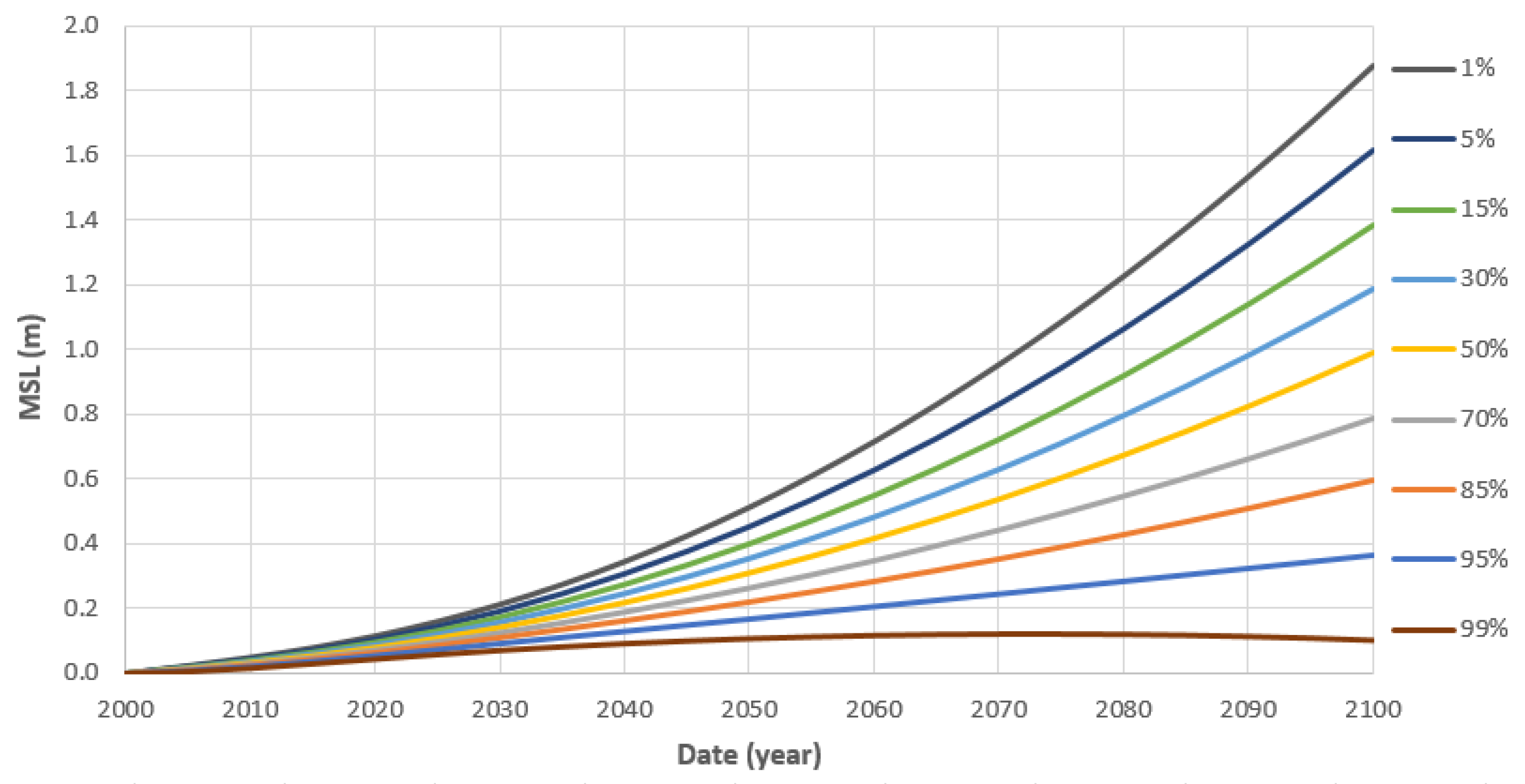
4.1. Relative SLR Models for the West Coast of Portugal Mainland (WCPM)

The Cascais and WCPM projections were denominated as FCUL (Faculty of Science of the Lisbon University) models and represented by the acronyms Mod.FC_0, Mod.FC_1, Mod.FC_2, and Mod.FC_3 (Figure 7). They were obtained by estimation models applied to Cascais TG data and, additionally, to East North Atlantic satellite altimetry MSL anomaly (NASA data center), near the WCPM, and to North Atlantic region (CNES), reduced with the estimated uplift velocity. Based on the observed regional MSL series and on different SLR acceleration estimates, these projections can be considered as the best relative SLR estimates for this region.

Mod.FC_0 was the only linear model (no acceleration) in which the rate of 4.1 mm/year was obtained from the most recent corrected daily MSL data series for the period from 2005 to 2016 (Table 1). Mod.FC_1 was estimated by a second order polynomial adjusted to a smoothed annual mean series for the period from 1980 to 2017 (acceleration in Table 3). Mod.FC_2 was divided into three sub-models: a model (a) in which the acceleration was estimated by a linear regression of an SL velocity series of Cascais MSL from 1976 to 2016; a model (b) in which the acceleration was estimated by finite differences of two consecutive SLR rates; and a model (c) in which the acceleration was estimated by finite differences from two consecutive rates of MSL anomalies of a region near Cascais, downloaded from NASA DAT (in Table 3). Finally, the Mod.FC_3 was divided into two sub-models: a model (a) in which the acceleration was computed by finite differences of two consecutive SLR rates estimated by linear regression applied to MSL anomaly from CNES satellite altimetry for the North Atlantic region; and a model (b) in which the acceleration was computed by finite differences of two consecutive SLR rates estimated by linear regression applied to MSL anomaly from NASA satellite altimetry for the East North Atlantic region near WCPM (in Table 3).

Table 4 lists the set of relative SLR empirical models for the region of the WCPM with the MSL projections for the middle (year 2050) and end (year 2100) of the 21st century, ordered by the increasing values of SLR at epoch 2100 and based on the accelerated model of Equation (1), with the initial velocity and acceleration parameters listed in the same table. The probability of each projection being exceeded at epoch 2100, computed from the normalized and adjusted PDF of the ensemble (in next section), is listed in the last column of Table 4.

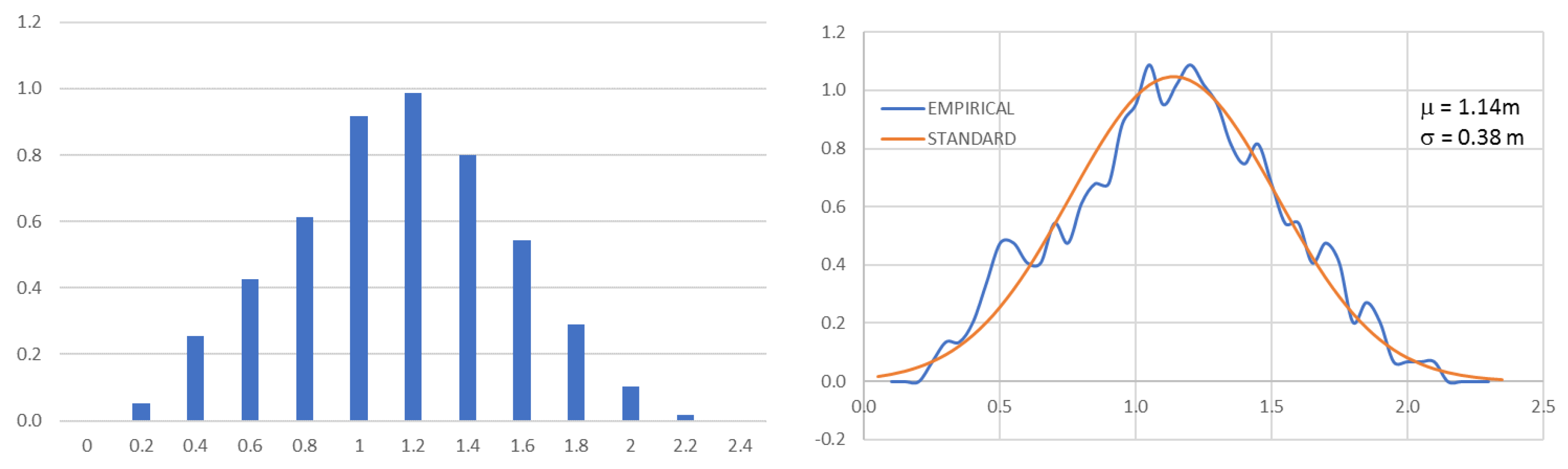
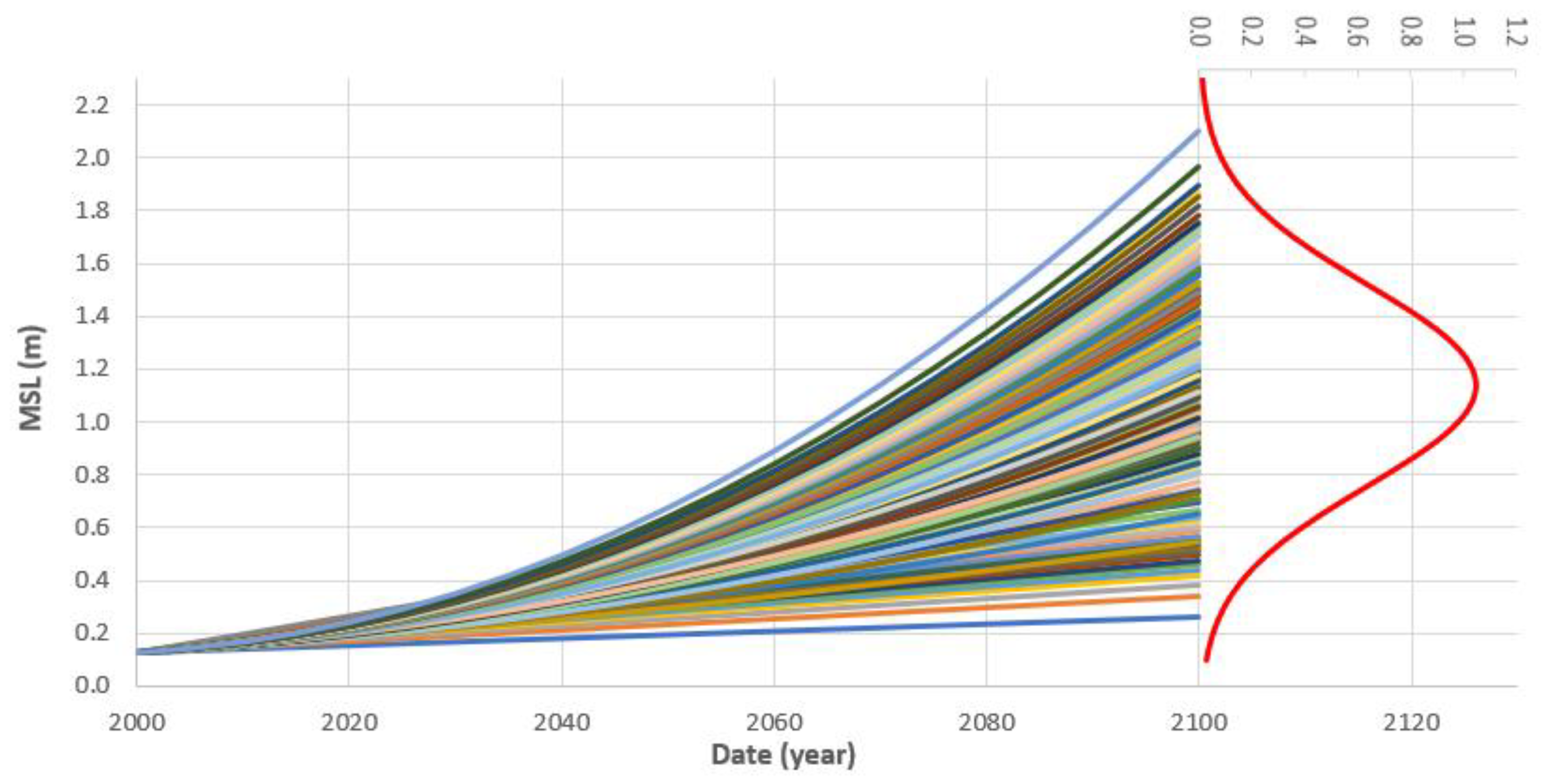
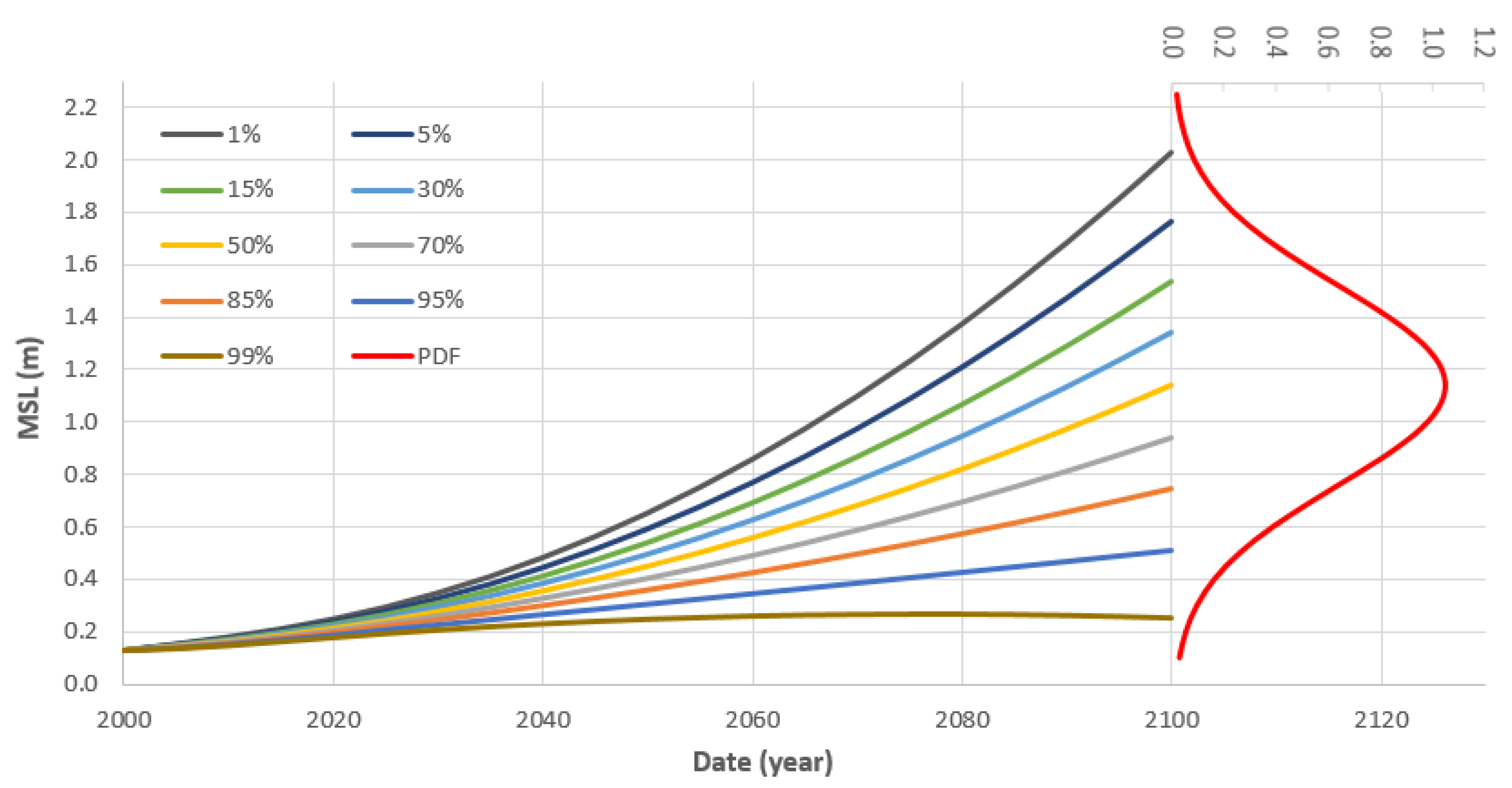
4.2. Probabilistic Ensemble of Empirical SLR Projections and Respective PDF

The objective of building up a probabilistic ensemble of SLR empirical models for the 21st century was based on the idea of defining a PDF for the 2100 projections, based on a considerable number of empirical estimations from MSL time series combined through a probabilistic ensemble. Due to this fact, each empirical model estimation has an associated uncertainty, specifically a certain probability to occur or a certain probability to be exceeded. Furthermore, given a PDF for the 2100 SLR, one can determine the exceeding probability of a certain SLR projection by its cumulative density function (CDF, the percentile function).

Considering all the acceleration estimations listed in Table 3 and the respective initial SLR velocities in the year 2000 (Table 4), a set of central SLR estimation can be derived, and the projection can be calculated from 2000 to 2100. Based on the general uncertainty propagation, the probability range of each centered estimation may be applied to any future time period, such as epoch 2100. Figure 8 shows the case of model Mod.FC_2b with extreme limits of probability (95% of confidence interval), superimposed with the respective PDF at epoch 2100 estimated by the uncertainty propagation. As shown in Figure 8, with a 2.5% and a 97.5% probability propagation, this calculation can be done for the propagation of any level of probability.

From each of the seven estimated projection models (Figure 7), an ensemble of n projected SLR probability curves, with a 5% of the interval, varying from 5 to 95%, with additional tail probabilities of 1 and 99%, can be generated. In total, an ensemble of 147 probabilistic projections was obtained, from which the relative frequency was analyzed and fitted to a normal probability density function (Figure 9). Based on the histogram of the relative frequency of MSL ensemble projections for 2100, it was possible to adjust a PDF function to the empirical relative frequency of the SLR projections ensemble for 2100. Figure 9 shows the histogram of the ensemble distribution (left) and the PDF adjusted to the empirical relative frequency (right).

Figure 10 shows the projection of relative SLR for the WCPM with the probabilistic ensemble of 147 runs. Superimposed to Figure 10 (plotted in vertical) is the PDF curve of the relative MSL distribution (from Figure 9) for the 2100 probabilistic ensemble.

Based on the PDF for the projected MSL at epoch 2100, the exceeding probability for each central projection can be computed. Table 4 lists the exceeding probability of empirical SLR projections, ranging from 94% for the lowest hazard projection of Mod.FC_0 to 8.8% for the highest hazard projection of Mod.FC_3b. The empirical projection with the highest probabilistic density was the model Mod.FC_2b, with 52.7% of exceeding probability.

Concerning to the PDF for MSL at epoch 2100 (Figure 11), the limits of 5% and 95% percentiles of the CDF corresponded to the values of 0.51 m and 1.77 m, and the 50% percentile, corresponding to the MSL ensemble average at epoch 2100, was estimated to be 1.14 m.

Table 5. Intervals of confidence for the WCPM relative SLR at epoch 2100 based on the cumulative density function of the PDF in Figure 9.

Confidence Level	Lower Limit (m)	Upper Limit (m)
30%	0.94	1.34
60%	0.74	1.54
90%	0.51	1.77
95%	0.39	1.89
99%	0.16	2.12

lists the lower and the upper limits for the confidence intervals of 30%, 60%, 90%, 95%, and 99% for the relative SLR at the WCPM. There was a 95% confidence that SLR at the WCPM might reach, at epoch 2100, any value in a range of 0.39 and 1.89 m.

To convert the ensemble of relative SLR to absolute SLR, to be comparable with IPCC RCP scenarios or with any other global or regional absolute model, the 2000 relative MSL for the local datum must be subtracted (13 cm relative to the national vertical reference of Cascais 1938) and reduced for the estimated uplift rate of 0.24 mm/year for the region applied to the initial SLR velocity at epoch 2000. The respective PDF must be shifted and scaled to be adjusted to the histogram of the respective relative frequency of the absolute SLR ensemble. Figure 12 shows the absolute SLR ensemble of the WCPM for the 21st century, relative to 2000 MSL; in this case, with an average absolute SLR of 0.99 m at epoch 2100, corresponding to the exceeding probability of 50%.

The probabilistic SLR projections, shown in Figure 12, can be compared to any global or regional model in order to estimate the respective exceeding probability. For instance, the SLR of RCP4.5 and RCP8.5 [1] at epoch 2100, in this probabilistic projection, corresponded to an exceeding probability of 88.4% and 74.5%, respectively, while the RCP2.6, concerning closely to Mod.FC_0, corresponded to a 92.5% of exceeding probability. On the other end, the used NOAA (National Oceanic and Atmospheric Administration) GSLR high-end projection models [19] (2 and 2.5 m of SLR), concerning to the presented PDF of the absolute SLR, corresponded to very low values of exceeding probability, 0.4% and 0.004%, respectively.

5. Conclusions

The present idea of running an ensemble of SLR projections for the West Coast of Portugal Mainland until the end of the 21st century, instead of projecting the best estimates based on empirical analyses or on global warming scenarios, intends to assess the probability and the respective cumulative density functions of an SLR ensemble. With such achievement, and through an adjusted PDF with a normal distribution, it is possible to estimate the exceeding probability of each SLR projection for 2100 based on MSL data, both relative and absolute SLR, as well as the limits of confidence intervals for a certain probability.

All the central projections of the empirical estimates were obtained by fitting a second order polynomial to the MSL data, running it for different data sets, different time period intervals, and by applying different numerical parametrization methods. The MSL present data is not yet influenced by the eventual collapse of the Greenland and Antarctica glaciers and ice caps. A future possibility of extreme ice melting acceleration, mainly from the West Antarctic Ice Sheet (WAIS), can only be represented by process-based models or semi-empirical projections. Therefore, extreme projections, such as those from the NOAA 2017 assessment report, which represent the possibility of such high-end GSLR scenarios at the end of the 21st century, have been pointed out by some authors as possible scenarios with higher probabilities as new data and new research have been published [5,19,20,21,22,23,24]. However, based on this current PDF estimation, those extreme scenarios still show very low exceeding probabilities, less than 1%.

With a different approach and based on the RCP8.5 scenario [25], it reached a similar PDF result for a GSLR projection for 2100. On comparing the high-end probability results of [25], the GSLR of 1.8 m obtained for the 5% of exceeding probability is very similar to 1.77 m obtained in this study. While in the present study, such absolute SLR of 1.8 m corresponded only to 1.7% of exceeding probability.

Reference [25] also provides a complete probability distribution of GSLR projection under the representative concentration pathways of IPCC and present a global set of local SLR projections. From their map representation of the medium RCP8.5 GSLR projection for 2100 (of 0.79 m), a value around 0.75–0.8 m for WCPM could be observed, denoting a low local vertical velocity, as it was calculated in this study. For the GSLR under RC8.5, the authors presented a very likely range of 0.52 to 1.21 m (90% of probability) and the respective high-end 99.9% percentile of 2.45 m. The 99.5% and 99.9% percentiles of GSLR projection from [26] resemble the percentiles of 98.8% (1.76 m) and 99.994% (2.45 m) of the present study, respectively.

Based on the values listed in Table 5 and on the PDF model of absolute SLR ensemble, there is 60% confidence that sea level at the WCPM will rise between 0.74 and 1.54 m with 50% of chance to reach 1.14 m at the end of the 21st century. Higher SLR, based on the right-end tail of the PDF, has lower probabilities for exceeding, with a 0.4% chance to reach 2 m (NOAA High scenario) until 2100 and only 0.004% chance to reach 2.5 m (NOAA Extreme scenario). These are SLR equivalent to [26] and higher than [25].

The present probability distribution, with a higher SLR range by the end of the 21st century as the projection made by [25,26], shows consistency with the most recent observations that show the polar ice melting acceleration [21,23,24] and with the possibility of extreme scenarios of [5,19].

The projections calculated in this study assume that SLR changes will be similar in the future, meaning that the acceleration estimates will not change until the end of the century. If SLR changes more rapidly in the future, showing higher acceleration values, due to rapid changes in the ice sheet dynamics, for instance, then these extrapolation-based projections will probably represent a conservative lower bound on future SLR. With such extreme scenarios, the second order polynomial models adjusted to current data will not fit future SLR estimations and different approaches, such as exponential, rather than accelerated, must then be applied.

References

1. IPCC. Climate Change 2013: The Physical Science Basis. Contribution of Working Group I to the Fifth Assessment Report of the Intergovernmental Panel on Climate Change; Stocker, T.F., Qin, D., Plattner, G.K., Tignor, M., Allen, S.K., Boschung, J., Nauels, A., Xia, Y., Bex, V., Midgley, P.M., Eds.; Cambridge University Press: Cambridge, UK; New York, NY, USA, 2013; 1535p. [Google Scholar]
2. Leuliette, E.W.; Nerem, R.S. Contributions of Greenland and Antarctica to global and regional sea level change. Oceanography 2016, 29, 154–159. [Google Scholar] [CrossRef]
3. Antunes, C.; Taborda, R. Sea level at Cascais Tide Gauge: Data, Analysis and Results. J. Coast. Res. 2009, SI 56, 218–222. [Google Scholar]
4. Antunes, C. Subida do Nível Médio do Mar em Cascais, revisão da taxa actual. In Actas das 4.as Jornadas de Engenharia Hidrográfica; Instituto Hidrográfico: Lisboa, Portugal, 2016; ISBN 978-989-705-097-8. [Google Scholar]
5. Hansen, J.; Sato, M.; Hearty, P.; Ruedy, R.; Kelle, M.; Masson-Delmotte, V.; Russell, G.; Tselioudis, G.; Cao, J.; Rignot, E.; et al. Ice melt, sea level rise and superstorms: evidence from paleoclimate data, climate modeling, and modern observations that 2 °C global warming could be dangerous. Atmos. Chem. Phys. 2016, 16, 3761–3812. [Google Scholar] [CrossRef] [Green Version]
6. Kopp, R.E.; DeConto, R.M.; Bader, D.A.; Hay, C.C.; Horton, R.M.; Kulp, S.; Oppenheimer, M.; Pollard, D.; Strauss, B.H. Evolving Understanding of Antarctic Ice-Sheet Physics and Ambiguity in Probabilistic Sea-Level Projections. Earth’s Future 2017, 5. [Google Scholar] [CrossRef]
7. Scambos, T.A.; Bell, R.E.; Alley, R.B.; Anandakrishnan, S.; Bromwich, D.H.; Brunt, K.; Oppenheimer, M.; Pollard, D.; Strauss, B.H. How much, how fast?: A science review and outlook for research on the instability of Antarctica’s Thwaites Glacier in the 21st century. Glob. Planet. Chang. 2017, 153, 16–34. [Google Scholar] [CrossRef]
8. Brown, T.P.; Caldeira, K. Greater future global warming inferred from Earth’s recent energy budget. Nature 2017, 552, 45–50. [Google Scholar] [CrossRef] [PubMed]
9. Jevrejeva, S.; Moore, J.C.; Grinsted, A.; Matthews, A.P.; Spada, G. Trends and acceleration in global and regional sea levels since 1807. Glob. Planet. Chang. 2014, 113, 11–22. [Google Scholar] [CrossRef] [Green Version]
10. Church, J.A.; White, N.J. Sea-level rise from the late 19th to the early 21st Century. Surv. Geophys. 2011, 32, 585–602. [Google Scholar] [CrossRef]
11. Church, J.A.; White, N.J. A 20th century acceleration in global sea-level rise. Geophys. Res. Lett. 2006, 33, L10602. [Google Scholar] [CrossRef]
12. Beckley, B.D.; Callahan, P.S.; Hancock, D.W.; Mitchum, G.T.; Ray, R.D. On the “Cal-Mode” Correction to TOPEX Satellite Altimetry and Its Effect on the Global Mean Sea Level Time Series. J. Geophys. Res. Oceans 2017, 122, 8371–8384. [Google Scholar] [CrossRef]
13. Nerem, R.S.; Beckley, B.D.; Fasullo, J.T.; Hamlington, B.D.; Masters, D.; Mitchum, G.T. Climate-change-driven accelerated sea-level rise detected in the altimeter era. Proc. Natl. Acad. Sci. USA 2018, 115, 2022–2025. [Google Scholar] [CrossRef] [PubMed]
14. Rhamstorf, S.; Foster, G.; Cazenave, A. Comparing climate projections to observations up to 2011. Environ. Res. Lett. 2012, 7, 044035. [Google Scholar] [CrossRef] [Green Version]
15. Cabral, J. Neotectónica em Portugal Continental. Inst. Geol. Min. Mem. 1995, 31, 265. [Google Scholar]
16. Figueiredo, P.M.; Cabral, J.; Rockwell, T.K. Recognition of Pleistocene marine terraces in the Southwest of Portugal (Iberian Peninsula): Evidences of regional Quaternary uplift. Ann. Geophys. 2013, 56. [Google Scholar] [CrossRef]
17. Peltier, W.R.; Argus, F.F.; Drummond, R. Space geodesy constrains ice-age terminal deglaciation: The global ICE-6G_C (VM5a) model. Annu. Rev. Earth Planet. Sci. 2015, 32, 111–149. [Google Scholar] [CrossRef]
18. Nerem, R.S.; Chambers, D.P.; Choe, C.; Mitchum, G.T. Estimating mean sea level change from the TOPEX and Jason altimeter missions. Mar. Geod. 2010, 33, 435–446. [Google Scholar] [CrossRef]
19. Sweet, V.W.; Kopp, R.E.; Weaver, P.C.; Obeysekera, J.; Horton, M.H.; Thieler, E.R.; Zervas, C. Global and Regional Sea Level Rise Scenarios for the United States; NOAA Technical Report NOS CO-OPS 083; NOAA: Silver Spring, MD, USA, 2017; 77p.
20. Seo, K.W.; Wilson, C.R.; Scambos, T.; Kim, B.M.; Waliser, D.E.; Tian, B.; Kim, B.-H.; Eom, J. Surface mass balance contributions to acceleration of Antarctic ice mass loss during 2003–2013. J. Geophys. Res. Solid Earth 2015, 120, 3617–3627. [Google Scholar] [CrossRef] [PubMed]
21. Martín-Español, A.; Zammit-Mangion, A.; Clarke, P.J.; Flament, T.; Helm, V.; King, M.A.; Luthcke, S.B.; Petrie, E.; Rémy, F.; Schön, N.; et al. Spatial and temporal Antarctic Ice Sheet mass trends, glacio-isostatic adjustment, and surface processes from a joint inversion of satellite altimeter, gravity, and GPS data. J. Geophys. Res. Earth Surf. 2016, 121, 182–200. [Google Scholar] [CrossRef] [PubMed] [Green Version]
22. Gardner, A.S.; Moholdt, G.; Scambos, T.; Fahnstock, M.; Ligtenberg, S.; van den Broeke, M.; Nilsson, J. Increase West Antarctic and unchanged East Antarctic ice discharge over the last 7 years. Cryosphere 2018, 12, 521–547. [Google Scholar] [CrossRef]
23. DeConto, R.M.; Pollard, D. Contributions of Antarctica to past and future sea-level rise. Nature 2016, 531, 591–610. [Google Scholar] [CrossRef] [PubMed]
24. Derksen, C.; Brown, R.; Mudryk, L.; Luojus, K.; Helfrich, S. Terrestrial Snow Cover. Arctic Report Card 2017. Available online: http://www.artic.noaa.gov/Report-Card (accessed on 5 March 2019).
25. Jevrejeva, S.; Grinsted, A.; Moore, J.C. Upper limit for sea level projections by 2100. Environ. Res. Lett. 2014, 9, 104008. [Google Scholar] [CrossRef] [Green Version]
26. Kopp, R.E.; Horton, R.M.; Little, C.M.; Mitrovica, J.X.; Oppenheimer, M.; Rasmussen, D.J.; Strauss, B.H.; Tebaldi, C. Probabilistic 21st and 22nd century sea-level projections at a global network of tide-gauge sites. Earth’s Future 2014, 2, 383–406. [Google Scholar] [CrossRef] [Green Version]
Figure 1. Location of Cascais tide gauge (TG). The old analog TG is operating since 1882, and the new acoustic TG with the digital record and with an internet connection is working since November 2003.
Jmse 07 00061 g001
Figure 2. Cascais TG secular series of monthly MSL, from 1882 to 2017, relative to the national vertical datum, and a moving average (MovAver) of the 10-year base period.
Jmse 07 00061 g002
Figure 3. Satellite altimetry GMSL anomalies from three international data centers, NASA, CNES (global and North Atlantic region), and CSIRO, superimposed to the Cascais MSL trend adjusted to 2000 reference.
Jmse 07 00061 g003
Figure 4. SLR rate of the 10-year moving average over the Cascais TG secular series (Figure 2).
Jmse 07 00061 g004
Figure 5. Daily mean sea level series (in meters) at Cascais TG, from 2000 to 2016, relative to the national vertical datum (in red), corrected from inverse barometric effect, vertical displacement, and mean seasonal oscillation, with a 6-months base period moving average (in blue). Analog TG data from Jan/2000 to Nov/2003 and from new acoustic TG data from Nov/2003 to Dec/2016.
Jmse 07 00061 g005
Figure 6. MSL of Cascais (in mm), modeled by a 20-years moving average of the secular series (Figure 2), adjusted to the GMSL from [9] by a rate of 0.43 mm/year (left graph) and fitted to the GMSL from [10] by a rate of 0.2 mm/year (right graph), both with rotation points at epoch 2000 and an adequate vertical shift to overlay the curves.
Jmse 07 00061 g006
Figure 7. Relative SLR projection models for the WCPM (in meters), superimposed with observed MSL at Cascais TG.
Jmse 07 00061 g007
Figure 8. Relative SLR projection of Mod.FC_2b (in meters) with probability limits of 95% confidence, superimposed with a PDF at epoch 2100 (fitted to the MSL y-axis) and observed MSL at Cascais TG, relative to the national vertical datum of Cascais 1938 (13 cm at epoch 2000).
Jmse 07 00061 g008
Figure 9. Histogram of the relative frequency of the ensemble projections at epoch 2100 (left) and the standard adjusted PDF (right) with a standard deviation of 38 cm.
Jmse 07 00061 g009
Figure 10. The ensemble of 147 relative SLR projections (in meters) for the 21st century of the WCPM, superimposed with PDF for 2100 (fitted to the MSL y-axis) and relative to the national vertical datum of Cascais 1938 (13 cm at epoch 2000).
Jmse 07 00061 g010
Figure 11. Relative SLR projections (in meters) for the 21st century of the WCPM, corresponding to a discrete set of percentiles, from 1 to 99% (probability of not being exceeded). The PDF curve is fitted to the MSL y-axis.
Jmse 07 00061 g011
Figure 12. Absolute SLR projections (in meters) for the 21st century of the WCPM, relative to 2000, and with the local vertical velocity removed, corresponding to a discrete set of percentiles, from 1 to 99%, or the probability of not be exceeded.
Jmse 07 00061 g012