Automatic Shoreline Detection from Eight-Band VHR Satellite Imagery


1
Department of Civil, Construction-Architecture and Environmental Engineering, University of dell’Aquila, 67100 L’Aquila, Italy
2
Department of Civil Construction and Environmental Engineering, Sapienza University of Rome, 00185 Rome, Italy
3
Department of Engineering, University of Perugia, 06125 Perugia, Italy
*
Author to whom correspondence should be addressed.
J. Mar. Sci. Eng. 2019, 7(12), 459; https://doi.org/10.3390/jmse7120459
Submission received: 12 November 2019
/
Revised: 7 December 2019
/
Accepted: 11 December 2019
/
Published: 13 December 2019
(This article belongs to the Special Issue Remote Sensing in Coastline Detection)
Abstract
:Coastal erosion, which is naturally present in many areas of the world, can be significantly increased by factors such as the reduced transport of sediments as a result of hydraulic works carried out to minimize flooding. Erosion has a significant impact on both marine ecosystems and human activities; for this reason, several international projects have been developed to study monitoring techniques and propose operational methodologies. The increasing number of available high-resolution satellite platforms (i.e., Copernicus Sentinel) and algorithms to treat them allows the study of original approaches for the monitoring of the land in general and for the study of the coastline in particular. The present project aims to define a methodology for identifying the instantaneous shoreline, through images acquired from the WorldView 2 satellite, on eight spectral bands, with a geometric resolution of 0.5 m for the panchromatic image and 1.8 m for the multispectral one. A pixel-based classification methodology is used to identify the various types of land cover and to make combinations between the eight available bands. The experiments were carried out on a coastal area with contrasting morphologies. The eight bands in which the images are taken produce good results both in the classification process and in the combination of the bands, through the algorithms of normalized difference vegetation index (NDVI), normalized difference water index (NDWI), spectral angle mapper (SAM), and matched filtering (MF), with regard to the identification of the various soil coverings and, in particular, the separation line between dry and wet sand. In addition, the real applicability of an algorithm that extracts bathymetry in shallow water using the “coastal blue” band was tested. These data refer to the instantaneous shoreline and could be corrected in the future with morphological and tidal data of the coastal areas under study.
1. Introduction
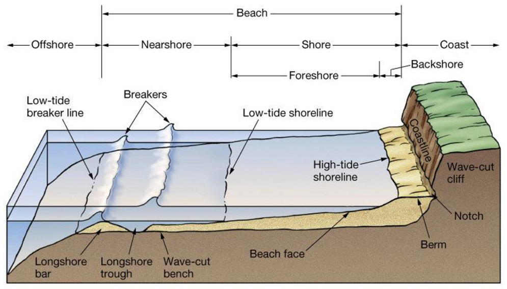
The coastal environment is an extraordinary natural and economic resource that is subject to continuous transformation. The coastal area is a highly dynamic system where erosion and deposition are influenced by various factors, including meteorological, biological, geological, and anthropogenic factors. The theoretical definition of coastline is merely the transition between the sea and the land [1,2,3]. In theory, the concept is very simple and intuitive, but its application is actually a complex task because of the temporal variability of the coastline itself. This variability develops on scales profoundly different, from instantaneous to secular variations, and it depends on various factors including wave motion, tides, winds, erosion, and deposition. It has been noted that the most significant and potentially incorrect assumption in many shoreline investigations is that the instantaneous shoreline represents “normal” or “average” conditions [3]. For this reason, what it is important to underline that what is obtained from survey in the field or remote sensing are generally indicators of the actual coastline [3,4,5]. According to some authors, there are three main subdivisions of coastline indicators: characteristics visible by an operator on an aerial or remote sensing image; intersection between a tidal datum and a digital terrain model or a coastal profile; and characteristics of multispectral images identified by automatic algorithms not necessarily visible to unaided operator [3]. In this work, we assess techniques associated with the third type by comparing them with each other and with those of the first type. The purpose of this work is to assess potentialities of automatic extraction of the coastline in a specific area particularly prone to erosion. In fact, the Abruzzo region (Italy) coastline has a length of 125 km, of which 26 km is high coasts and 75 km is sandy coasts; the latter, therefore, are 80% of the entire coastline, and more than 50% are under erosion effects. The study of this paper was conducted on the sandy coast of Ortona (Abruzzo Region), in which three erosion phenomena have been reported on the coast, four active landslides have effects on the coast, and three landslide crags occur on the sea [6]. For this reason, according to the guidelines for the defense of the coast against erosion and the effects of climate change [7], one of the fundamental elements of a coastal information system is the extraction of the shoreline. A specific assessment on these areas has not yet been carried out and its results will be very useful for the continuation of the research and for the applications that can be implemented. It is important to note that what is extracted are indicators of the coastline and not the coastline itself (Figure 1).
In this work, after a brief illustration of the state of the art on the techniques of extraction of the coastline, we will introduce the materials and methods used for the experiments illustrated. Subsequently, the results obtained by them will be shown in the following specific paragraph, while the conclusions and possible future developments will be discussed together in the last paragraph of the paper.
2. State of the Art of Instant Shoreline Survey
From what has been said previously, it is easy to understand that the relief of the instantaneous shoreline is a complex feature due to the intrinsic dynamism of the shoreline itself. A wide variety of methodologies have been used [7,8,9,10] that can be summarized mainly in the following:
- Photogrammetry/videography from airplane or UAV: In the first case, this is a matter of using the well-known techniques of photogrammetry from single acquisitions of aerial images that are currently almost all digital images; digital cameras can easily acquire films that can be treated with classical photogrammetric algorithms or with new approaches such as structure from motion (SFM) [11,12].
- Terrestrial video systems: These are fixed camera systems which acquire at fixed time-intervals and which are composed of several cameras distributed along the coast with acquisition angles of up to 180 degrees. This technique produces oblique images that must be orthorectified [13].
- Earth and satellite geomatic surveys: These are the classic surveys with instruments such as GPS/GNSS and total stations, levels that have a remarkable accuracy but can detect a limited number of points at different times.
- Terrestrial and aerial lidar survey that can reconstruct both the surfaces of water and ground [12] or penetrate shallow water.
- Remote sensing from satellite: It should be noted that with the development of remote sensing, shoreline detection is mainly achieved by image processing [14]. The availability of multispectral satellite images at very high resolution (VHR) allows, in fact, acquisition in a short time and simultaneously of long stretches of coast. The geometric accuracies of submetric to decimetric order are absolutely compatible with the specific application and the availability of different bands allows semi-automatic or automatic approaches [15,16,17] such as those proposed in this paper.
3. Materials and Methods
3.1. The WorldView-2 Satellite
The WorldView-2 satellite, launched in October 2009, added to the already existing constellation of commercial satellites DigitalGlobe [18], already formed at the time by the satellites WorldView-1 (launched in 2007) and QuickBird (launched in 2001). Its planned mission duration was 7.25 years, but it has just turned 10 years old. WorldView-2 operates at an altitude of 770 km with an inclination of 97.2° for a maximum orbital period of 100 min. It is equipped with instrumentation that allows it to collect high-resolution multispectral images and stereoscopic images.
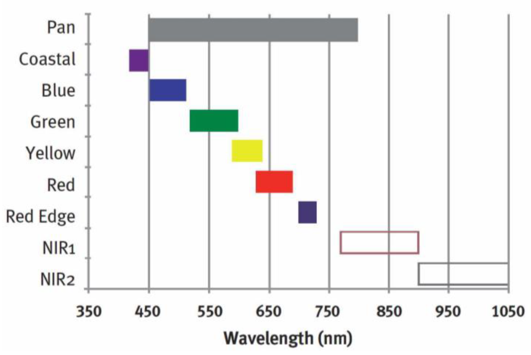
The maximum ground resolution of WorldView-2 in the panchromatic band is 46 cm, while in the multispectral band it is 1.8 m, however the distribution and use of images with a resolution greater than 50 cm in the panchromatic band and 2 meters in the multispectral band is subject to approval by the US government. The high spatial resolution allows discrimination of details, such as vehicles, shallows, and individual trees in an orchard, while the high spectral resolution provides detailed information on different areas, such as road surface quality, sea depth, and plant health. The images are taken in eight spectral bands. In addition to the four standard bands (blue, green, red, and near infrared), WorldView-2 includes four new bands at 1.8 m resolution: coastal blue, yellow, red edge, and near infrared-2 (Figure 2).
3.2. Test Site
The images used in this project are multispectral WorldView-2 images representing a part of the coast of the city of Ortona (Italy) (Figure 3). For this specific project, the tests were performed on a bundle of panchromatic and multispectral images acquired simultaneously in June. To be sure that the variability of the results depended only on the algorithm used in the various tests performed and not on factors due to different inclination of the image or the sun, the tests were all repeated on the same bundle of images. The images were processed entirely on the whole scene, but the results were highlighted on a single profile that was considered significant and representative of the tests on the whole scene. Ortona is a seaside town overlooking the Mediterranean Sea, more specifically, the Adriatic Sea (Figure 4); the coast is high and rocky in the southern part while it is low and sandy in the central northern part. The inner part of the city of Ortona is partly flat and partly hilly.
In order to evaluate the possibilities of automatic extraction of the coastline (understood as an instantaneous shoreline as visible on satellite images), different combinations of algorithms on different spectra of the available images were tested and are illustrated below. The tests were developed in the ENVI 5.5 environment [19].
4. Experimentation and Results
4.1. Analysis of Individual Bands and Band Combinations
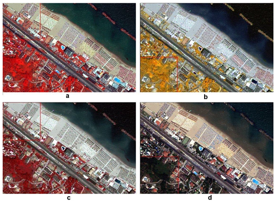
The first step in such an analysis is almost always pansharpening [20]; this operation creates a single multilayer image combining the panchromatic image of higher spatial resolution (in this case 50 cm) with the various multispectral levels (Figure 5) that have more thematic information but lower geometric resolution (in this case 1.8 m). Several algorithms have been developed to optimize pansharpening, and the comparison between them is at the center of a scientific debate [21,22,23].
In this experiment, Graham Smith’s algorithm [24] was used because it has demonstrated to be the most reliable and accurate in previous studies [21,23]. This algorithm first calculates the weights of the single bands with the following equations:
where OT is optical transmittance and SR is the spectral response of the various bands with their wavelengths. Once the specific weights have been calculated, the simulated band is created using the following equation:
Once the pansharpening has been undertaken (Figure 6), it is possible to start to perform operations on the single bands or on combinations of them.
Among the most used indices in the combination of the bands there is undoubtedly the vegetation index (NDVI) and the normalized difference water index (NDWI). Both these indices have been tested because they automatically highlight the instantaneous shoreline, showing a remarkable discontinuity approaching it. The NDVI is a well-known index used to study vegetation, exploiting the different response between the near-infrared band and the red band:
In vegetation studies, it is widely used because it allows to distinguish the plants that correctly perform the chlorophyll synthesis from those that do not. In vegetation applications it provides a dimensionless value between −1 and 1 but can also be usefully used for the coastline studies because the proximity of the shoreline assumes values between –0.5 and −0.1.
The second index, the NDWI, has been studied just to distinguish the areas covered by water from those that are not; it is actually very similar to the NDVI but uses the green band instead of the red one, and its formulation is in fact the following:
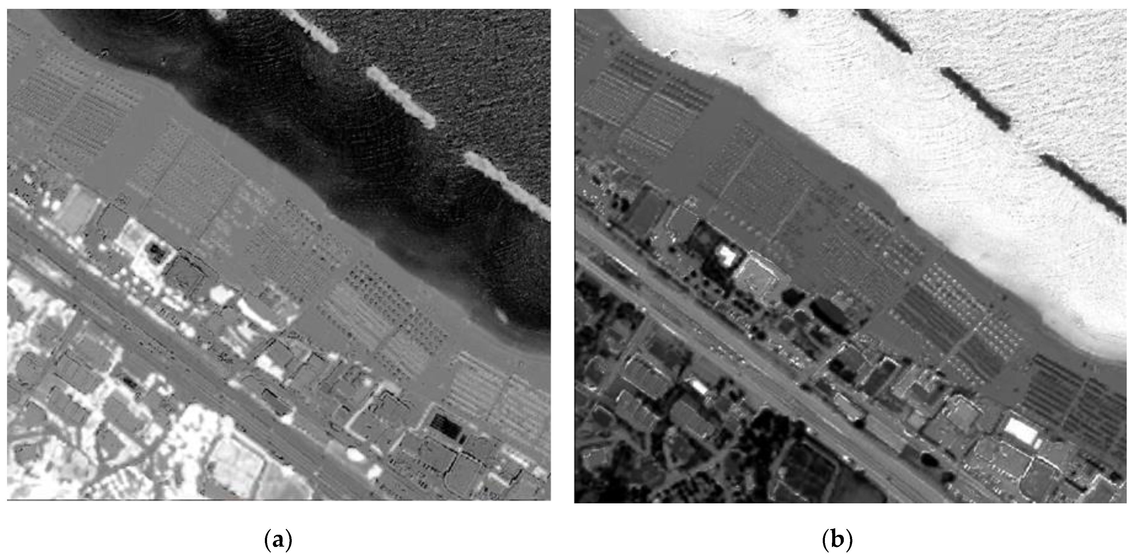
Using the NDWI, the areas covered by water are characterized by positive values of the index while vegetation and bare soil usually show negative values. Dry sand, because of its high reflectance in the green band, usually shows positive values that are close to zero (Figure 7).
4.2. Automatization of Water and Vegetation Detection
Below, we will analyze the results that can be obtained with the various algorithms available by comparing them on a specific profile that showed the characteristic aspects of a high coast and a sandy coast. On the panchromatic image, the sea/beach limits have been vectorized on the screen by an expert photo-interpreter. The purpose of this research is in fact to verify how efficient and accurate the automatic algorithms can be compared to the manual vectorization that is currently used to extract the instantaneous shoreline from satellite images. The ground surveys, already tested in previous researches [14], are certainly more accurate than those obtained from satellite images, but on sandy shores they cannot acquire the entire line of the instantaneous shoreline at the same time as it is visible on a satellite image and, therefore, are not directly comparable with them. The beach/sea and sea/detached-breakwater limits vectorized by the operator on the profile have been considered as reference for all the algorithms tested and are highlighted by the dashed lines in final comparison of the various algorithms tested. Considering that the pixel size in panchromatic is about 50 cm, the differences between the beach/sea limits vectorized by the operator with those extracted automatically equal to or less than 50 cm were not considered significant.
In this way, it will be possible to estimate the accuracy of the various algorithms, both in absolute and relative terms. What was important to observe was the possible discontinuity in the digital numbers of the images after the processing with the various algorithms; in fact, the edge-detector algorithms can easily trace border vector lines in the presence of sharp discontinuities.
The profile executed on the image processed with the NDVI algorithm shows a strong variation in slope at the boundaries of sea/beach and sea/detached-breakwater (Figure 8).
The spectral angle mapper (SAM) and matched filtering (MF) algorithms are very similar to NDVI but use all four bands (R, G, B, IR). SAM determines the spectral similarity between two spectra by calculating the angle between the spectra and treating them as vectors in a space with dimensionality equal to the number of bands. This technique, when used on calibrated reflectance data, is relatively insensitive to illumination and albedo effects [25]. MF, instead, maximizes the response of the known endmember and suppresses the response of the composite unknown background, thus matching the known signature [26] (Figure 9).
The MF/SAM ratio has the characteristic of highlighting the transition from wet to dry sand that is revealed by a rapid change in the slope of the curve that represents it (Figure 10).
The availability of the coastal blue band allowed us to exploit the algorithm called relative depth, developed by Stumpf and Holderied [27]. Using combinations of all bands provided a value of water depth up to about 14 m deep.
As the name of the algorithm says, the depth is relative, and in fact the values vary between 0 and 1; for bathymetric studies, therefore, control points measured to calibrate the model are required (Figure 11 and Figure 12).
Comparing the various algorithms (Figure 13), it can be observed that they all show a marked discontinuity near the actual line of contact between sea and land; it is important to note that values in the y direction are reported for every specific algorithm so are not directly comparable, but what is important to observe is the discontinuity in the different trends. Among them, the most efficient and accurate algorithm seems to be the relative depth, because the discontinuity shown at the passage between water and land is the deepest, showing an almost vertical trend; on the other hand, it can be noted that, at the pier, the deepness algorithm shows more than one discontinuity, making it more difficult to identify the two actual sea/detached-breakwater crossings. For this reason it was decided to deepen the study of this algorithm using the coastal blue band.
4.3. The Coastal Blue Band and the Relative Depth Algorithm
The results obtained using the relative depth algorithm have suggested that it could be further enhanced to deepen the study by using the coastal blue band, although this is not present on all satellite platforms. One can get useful information not only on the coast but also on the first meters of the seabed thanks to its ability to penetrate clear water. For the study of the coastline, we have observed how the algorithm assumes a value of zero in the presence of land emersion (Figure 14) while reconstructing the profile of the seabed moving to the sea.
However, the depth is relative, and therefore some known depths are necessary to transform the relative depths into absolute values. The only official data on the depths in this area are those released by the Military Geographic Institute (IGMI), collected with various techniques and accuracy. The correct calibration of the results of the algorithms would require more accurate measurements taken at the same time as the acquisition of the image. The data provided by the IGM only allow us to make a rough evaluation of the trends of the algorithm itself. In this way, we obtained the absolute depth profile (Figure 15).
The general trend is very similar to the expected one (Figure 16), also highlighting the differences in altitude near the detached breakwater. Despite the use of a median filter, some circular bathymetric curves are observed that might not respond to real morphologies. This could be due to the high detail of the information or to some bias of the algorithm; to be able to evaluate with certainty the performance of the algorithm, it would also be necessary to have a survey with greater accuracy (for example, side scan sonar) performed at the same time as the acquisition of the image.
4.4. Supervised Multispectral Classification
To complete the framework of the experiments, a supervised multispectral classification was also performed using the maximum likelihood algorithm; for this purpose, several regions of interest (ROI) were defined, including four building classes and three vegetation classes (Figure 17).
The result obtained from such a classification was a new raster file in which, in each pixel, the digital number corresponding to the class of land cover to which the pixel itself has been associated is reported (Figure 18). This classification works equally well in the division of the various types of buildings and vegetation as well as with the separation of dry sand and wet sand. We compared the instantaneous shoreline thus obtained with the only official one available, that is the one reported in the regional map scale 1:5000, aware of the shifts due to different period, time, and phase of the waves, however, finding a good agreement that can only confirm that the coastline in this area has not undergone major changes.
5. Conclusions and Further Developments
The purpose of this project was to identify the most efficient procedure for automatically extracting the instantaneous shoreline in sandy coasts of the Abruzzo region that are affected by severe erosion problems. What was important to observe were the possible discontinuities in the digital numbers of the images after treatment with the various algorithms; in fact, once any discontinuities have been identified, the edge-detector functions are able to easily draw border vector lines on the same discontinuities. Therefore, different algorithms have been tested and their trends on the sea/beach passage have been examined, comparing them with the limits identified on the same image by an experienced photogrammetric operator.
The algorithm that showed a trend with more sharp discontinuities and coinciding with those identified by the operator was the relative depth. However, this algorithm showed more discontinuities than those observable on the image at the pier. For this reason, it was subsequently experimented with to see if it was possible to improve the results using the coastal blue band. It has been verified that the costal blue with the relative depth eliminates the problem of the multiple detections. It can be deduced that the most accurate results for this specific application are obtained with the relative depth algorithm using the coastal blue band of the WorldView 2 satellite.
As far as the use of the same algorithm for the evaluation of bathymetry is concerned, it is necessary to have precise, punctual measurements to calibrate it and measurements such as side scan sonar to verify it; both should be carried out at the same time as the acquisition of the image to be significant.
Author Contributions
Supervision, M.A., V.B., R.B. and F.R.; Methodology, M.A., V.B., R.B. and F.R.; Investigation, M.A., V.B., R.B. and F.R.; Writing—Review and editing, V.B., R.B. and F.R.
Funding
This research received no external funding.
Conflicts of Interest
The authors declare no conflict of interest.
References
- Dolan, R.; Hayden, B.P.; May, P.; May, S. The reliability of shoreline change measurements from aerial photographs. Shore Beach 1980, 48, 22–29. [Google Scholar]
- Cervino, R.; Ivaldi, R.; Surace, L. Il ruolo dell’Istituto idrografico della Marina nel monitoraggio costiero. In Proceedings of the 3rd Symposium Il Monitoraggio Costiero Mediterraneo: Problematiche e Tecniche di Misura, Livorno, Italy, 15–17 June 2010. [Google Scholar]
- Boak, E.H.; Turner, I.L. Shoreline definition and detection: A review. J. Coast. Res. 2005, 21, 688–703. [Google Scholar] [CrossRef] [Green Version]
- Aguilar, F.J.; Fernández, I.; Pérez, J.L.; López, A.; Aguilar, M.A.; Mozas, A.; Cardenal, J. Preliminary results on high accuracy estimation of shoreline change rate based on coastal elevation models. Int. Arch. Photogramm. Remote Sens. Spat. Inf. Sci. 2010, 33, 986–991. [Google Scholar]
- Klein, M.; Lichter, M. Monitoring changes in shoreline position adjacent to the Hadera power station, Israel. Appl. Geogr. 2006, 26, 210–226. [Google Scholar] [CrossRef]
- Progetto Preliminare Della Costa Teatina—Fenomeni Erosivi Della Fascia Costiera. Available online: http://www.provincia.chieti.it/flex/cm/pages/ServeAttachment.php/L/IT/D/2%252F4%252F4%252FD.d367c153fd7837fd72ca/P/BLOB%3AID%3D3926/E/pdf (accessed on 28 October 2019).
- MATTM-Regioni. Linee Guida per la Difesa Della Costa dai Fenomeni di Erosione e Dagli Effetti dei Cambiamenti Climatici. Versione 2018—Documento Elaborato dal Tavolo Nazionale sull’Erosione Costiera; MATTM-Regioni con il Coordinamento Tecnico di ISPRA: Rome, Italy, 2018; 305p. [Google Scholar]
- Klemas, V. Airborne Remote Sensing of Coastal Features and Processes: An Overview. J. Coast. Res. 2013, 29, 239–255. [Google Scholar] [CrossRef]
- Costantino, D.; Angelini, M.G. Thermal monitoring using an ASTER image. J. Appl. Remote Sens. 2016, 10, 46031. [Google Scholar] [CrossRef]
- Tarig, A. New Methods for Positional Quality Assessment and Change Analysis of Shoreline Features. Ph.D. Thesis, School of the Ohio State University, Columbus, OH, USA, 2003. [Google Scholar]
- Ullman, S. The Interpretation of Structure from Motion, The Royal Society. University of Southampton. 1979. Available online: https://www.jstor.org/stable/77505 (accessed on 12 December 2019).
- Troisi, S.; Baiocchi, V.; Del Pizzo, S.; Giannone, F. A prompt methodology to georeference complex hypogea environments. Int. Arch. Photogramm. Remote Sens. Spat. Inf. Sci. 2017, 42, 639–644. [Google Scholar] [CrossRef] [Green Version]
- Pugliano, G.; Robustelli, U.; Di Luccio, D.; Mucerino, L.; Benassai, G.; Montella, R. Statistical Deviations in Shoreline Detection Obtained with Direct and Remote Observations. J. Mar. Sci. Eng. 2019, 7, 137. [Google Scholar] [CrossRef] [Green Version]
- Palazzo, F.; Latini, D.; Baiocchi, V.; Del Frate, F.; Giannone, F.; Dominici, D.; Remondiere, S. An application of COSMO-Sky Med to coastal erosion studies. Eur. J. Remote Sens. 2012, 45, 361–370. [Google Scholar] [CrossRef] [Green Version]
- Toure, S.; Diop, O.; Kpalma, K.; Maiga, A.S. Shoreline Detection using Optical Remote Sensing: A Review. Isprs Int. J. Geo. Inf. 2019, 8, 75. [Google Scholar] [CrossRef] [Green Version]
- Dai, C.; Howat, I.; Larour, E.; Husby, E. Coastline extraction from repeat high resolution satellite imagery. Remote Sens. Environ. 2019, 229, 260–270. [Google Scholar] [CrossRef]
- Dominici, D.; Zollini, S.; Alicandro, M.; Della Torre, F.; Buscema, P.M.; Baiocchi, V. High Resolution Satellite Images for Instantaneous Shoreline Extraction Using New Enhancement Algorithms. Geosciences 2019, 9, 123. [Google Scholar] [CrossRef] [Green Version]
- WorldView-2 Satellite Sensor. Available online: https://www.satimagingcorp.com/satellite-sensors/worldview-2/ (accessed on 12 December 2019).
- Available online: https://www.harrisgeospatial.com/Support/Maintenance-detail/ArtMID/13350/ArticleID/23403/Whats-New-ENVI174-55 (accessed on 12 December 2019).
- Maglione, P.; Parente, C.; Vallario, A. Coastline extraction using high resolution WorldView-2 satellite imagery. Eur. J. Remote Sens. 2014, 47, 685–699. [Google Scholar] [CrossRef]
- Baiocchi, V.; Bianchi, A.; Maddaluno, C.; Vidale, M. Pansharpening techniques to detect mass monument damaging in Iraq. Int. Arch. Photogramm. Remote Sens. Spat. Inf. Sci. 2017, XLII-5/W1, 121–126. [Google Scholar] [CrossRef] [Green Version]
- Parente, C.; Pepe, M. Influence of the weights in IHS and Brovey methods for pan-sharpening WorldView-3 satellite images. Int. J. Eng. Technol. 2017, 6, 71. [Google Scholar] [CrossRef] [Green Version]
- Vivone, G.; Alparone, L.; Chanussot, J.; Dalla Mura, M.; Garzelli, G.; Licciardi, A.; Restaino, R.; Wald, L. A critical comparison among pansharpening algorithms. IEEE Trans. Geosci. Remote Sens. 2015, 53, 2565–2586. [Google Scholar] [CrossRef]
- Maurer, T. How to pan-sharpen images using the gram-schmidt pan-sharpen metho—A recipe. Int. Arch. Photogramm. Remote Sens. Spat. Inf. Sci. 2013, XL-1/W1, 239–244. [Google Scholar] [CrossRef] [Green Version]
- Kruse, F.A.; Lefkoff, A.B.; Boardman, J.B.; Heidebrecht, K.B.; Shapiro, A.T.; Barloon, P.J.; Goetz, A.F.H. The Spectral Image Processing System (SIPS)—Interactive Visualization and Analysis of Imaging spectrometer Data. Remote Sens. Environ. 1993, 44, 145–163. [Google Scholar] [CrossRef]
- Ferrier, G. Application of Imaging Spectrometer Data in Identifying Environmental Pollution Caused by Mining at Rodaquilar, Spain. Remote Sens. Environ. 1999, 68, 125–137. [Google Scholar] [CrossRef]
- Stumpf, R.P.; Holderied, K.; Sinclair, M. Determination of water depth with high-resolution satellite imagery over variable bottom types. Limnol. Oceanogr. 2003, 1. [Google Scholar] [CrossRef]
Figure 1.
Indicators of the coastline.

Figure 2.
WorldView-2 spectral bands.

Figure 3.
The test site area on the Adriatic coast (red circle).

Figure 4.
Test site area: the yellow box is the area shown in the following figures.

Figure 5.
Some band combinations: (a) NIR1-G-B; (b) NIR1-Rededge-R; (c) R-G-B; (d) Rededge-R-Y.

Figure 6.
The pansharpening process: (a) MultiSpectral; (b) Panchromatic; (c) PanSharpened.

Figure 7.
(a) Normalized difference vegetation index (NDVI) and (b) normalized difference water index (NDWI) processed images in gray scale.
Figure 7.
(a) Normalized difference vegetation index (NDVI) and (b) normalized difference water index (NDWI) processed images in gray scale.

Figure 8.
NE to SW NDVI profile path on (a) RGB and (b) NDVI processed images; (c) NE to SW NDVI profile, distances on the x-axis are expressed in metres. The profile trend shows sharp discontinuities at sea/land limits.
Figure 8.
NE to SW NDVI profile path on (a) RGB and (b) NDVI processed images; (c) NE to SW NDVI profile, distances on the x-axis are expressed in metres. The profile trend shows sharp discontinuities at sea/land limits.

Figure 9.
NE to SW matched filtering (MF) muddy profile path on (a) RGB and (b) MF muddy processed images; (c) NE to SW MF muddy profile, distances on the x-axis are expressed in metres. The profile trend does not show sharp discontinuities at sea/land limits.
Figure 9.
NE to SW matched filtering (MF) muddy profile path on (a) RGB and (b) MF muddy processed images; (c) NE to SW MF muddy profile, distances on the x-axis are expressed in metres. The profile trend does not show sharp discontinuities at sea/land limits.

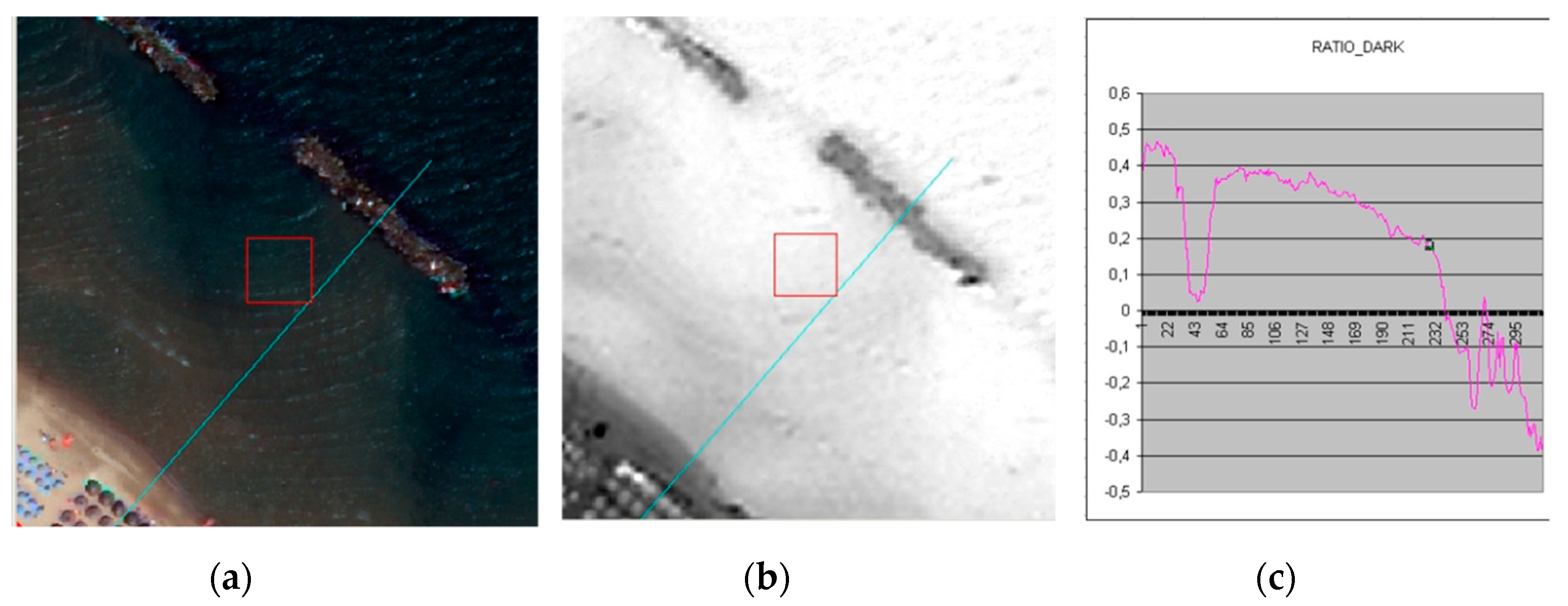
Figure 10.
NE to SW MF/spectral angle mapper (SAM) profile path on (a) RGB and (b) MF/SAM processed images; (c) NE to SW MF/SAM profile, distances on the x-axis are expressed in metres. The profile trend shows visible discontinuities at sea/land limits.
Figure 10.
NE to SW MF/spectral angle mapper (SAM) profile path on (a) RGB and (b) MF/SAM processed images; (c) NE to SW MF/SAM profile, distances on the x-axis are expressed in metres. The profile trend shows visible discontinuities at sea/land limits.

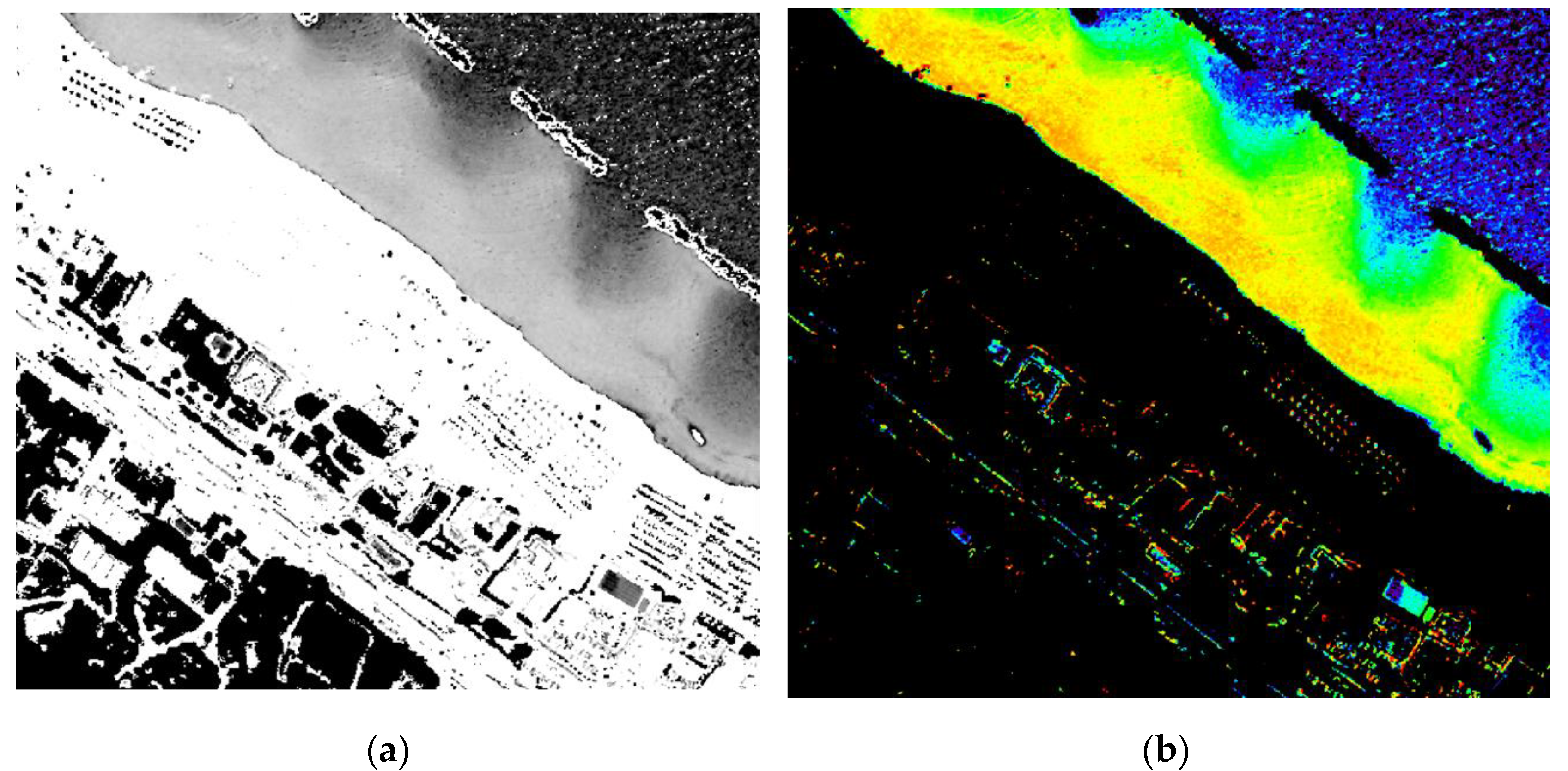
Figure 11.
Relative depth algorithm results represented in (a) gray and (b) pseudocolor scales.

Figure 12.
NE to SW relative depth profile path on (a) RGB and (b) relative depth processed images; (c) NE to SW relative depth profile, distances on the x-axis are expressed in metres. The profile trend shows almost vertical discontinuities at sea/land limits.
Figure 12.
NE to SW relative depth profile path on (a) RGB and (b) relative depth processed images; (c) NE to SW relative depth profile, distances on the x-axis are expressed in metres. The profile trend shows almost vertical discontinuities at sea/land limits.

Figure 13.
Comparison of the different algorithms on the same profile, black dashed lines are the actual water/ground limits (distances in the x direction are in meters along the profile, values in the y direction are reported for every specific algorithm so are not directly comparable).
Figure 13.
Comparison of the different algorithms on the same profile, black dashed lines are the actual water/ground limits (distances in the x direction are in meters along the profile, values in the y direction are reported for every specific algorithm so are not directly comparable).

Figure 14.
Detail of relative depth algorithm results using coastal blue band; on (a) the profile trac, on (b) the resulting profile were open water is on the right, distances in the x direction are in meters along the profile.
Figure 14.
Detail of relative depth algorithm results using coastal blue band; on (a) the profile trac, on (b) the resulting profile were open water is on the right, distances in the x direction are in meters along the profile.

Figure 15.
“Absolute depth” profile: along the y direction is the absolute depth and along the x direction is the progressive distance; all distances are in meters and open water is on the right.
Figure 15.
“Absolute depth” profile: along the y direction is the absolute depth and along the x direction is the progressive distance; all distances are in meters and open water is on the right.

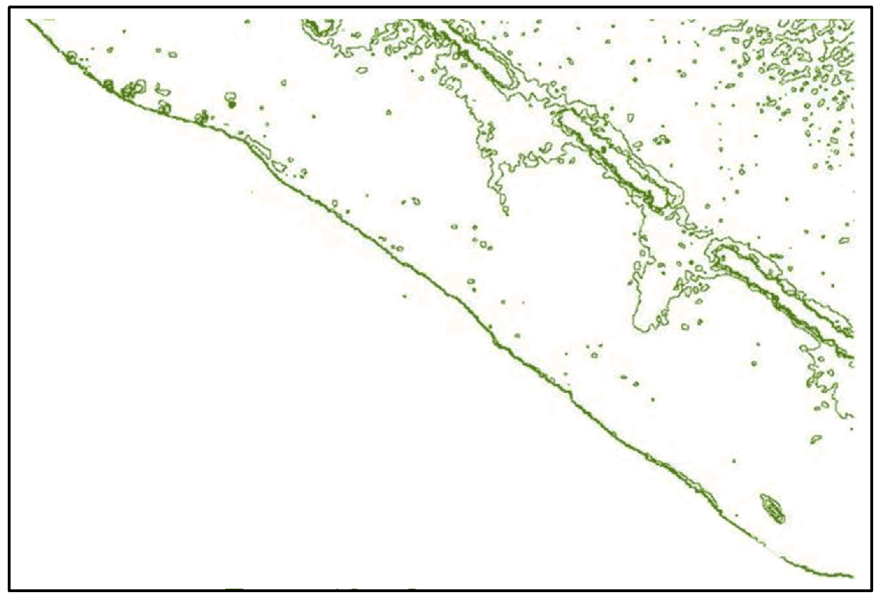
Figure 16.
“Absolute depth” bathymetric lines; open water is on the right.

Figure 17.
Detail of a vegetated area on RGB image on (a) and corresponding classification classes on (b).
Figure 17.
Detail of a vegetated area on RGB image on (a) and corresponding classification classes on (b).

Figure 18.
(a) Pansharpened image; (b) classified image; (c) classes legend.

© 2019 by the authors. Licensee MDPI, Basel, Switzerland. This article is an open access article distributed under the terms and conditions of the Creative Commons Attribution (CC BY) license (http://creativecommons.org/licenses/by/4.0/).
Share and Cite
MDPI and ACS Style
Alicandro, M.; Baiocchi, V.; Brigante, R.; Radicioni, F. Automatic Shoreline Detection from Eight-Band VHR Satellite Imagery. J. Mar. Sci. Eng. 2019, 7, 459. https://doi.org/10.3390/jmse7120459
AMA Style
Alicandro M, Baiocchi V, Brigante R, Radicioni F. Automatic Shoreline Detection from Eight-Band VHR Satellite Imagery. Journal of Marine Science and Engineering. 2019; 7(12):459. https://doi.org/10.3390/jmse7120459
Chicago/Turabian StyleAlicandro, Maria, Valerio Baiocchi, Raffaella Brigante, and Fabio Radicioni. 2019. "Automatic Shoreline Detection from Eight-Band VHR Satellite Imagery" Journal of Marine Science and Engineering 7, no. 12: 459. https://doi.org/10.3390/jmse7120459
Note that from the first issue of 2016, this journal uses article numbers instead of page numbers. See further details here.