Time Domain Modeling of Propeller Forces due to Ventilation in Static and Dynamic Conditions


1
SINTEF Ocean, Otto Nielsens vei 10, 7052 Trondheim, Norway
2
Kongsberg University Technology Centre “Performance in a Seaway” at NTNU, N-7491 Trondheim, Norway
3
Department of Marine Technology, Faculty of Engineering Science and Technology, Norwegian University of Science and Technology, N-7491 Trondheim, Norway
*
Author to whom correspondence should be addressed.
J. Mar. Sci. Eng. 2020, 8(1), 31; https://doi.org/10.3390/jmse8010031
Submission received: 5 November 2019
/
Revised: 19 December 2019
/
Accepted: 23 December 2019
/
Published: 9 January 2020
(This article belongs to the Special Issue Selected Papers from the Sixth International Symposium on Marine Propulsors)
Abstract
:This paper presents experimental and theoretical studies on the dynamic effect on the propeller loading due to ventilation by using a simulation model that generates a time domain solution for propeller forces in varying operational conditions. For ventilation modeling, the simulation model applies a formula based on the idea that the change in lift coefficient due to ventilation computes the change in the thrust coefficient. It is discussed how dynamic effects, like hysteresis effects and blade frequency dynamics, can be included in the simulation model. Simulation model validation was completed by comparison with CFD (computational fluid dynamics) calculations and model experiments. Experiments were performed for static and dynamic (heave motion) conditions in the large towing tank at the SINTEF Ocean in Trondheim and in the Marine Cybernetics Laboratories at NTNU (Norwegian University of Science and Technology). The main focus of this paper is to explain and validate the prediction model for thrust loss due to ventilation and out of water effects in static and dynamic heave conditions.
1. Introduction
Ventilation is the phenomenon by which air is drawn on structures operating below the free surface, such as hydrofoils, rudders, and propellers. Propeller ventilation might happen when the propeller is coming close to the free surface and air is drawn to it, or when the blades are piercing the free surface and the air is sucked down to the below-water parts of the propeller. Propeller ventilation leads to a sudden and large loss of propeller thrust and torque, which might lead to propeller racing and possibly damaging dynamic loads, as well as noise and vibrations. Ventilation typically occurs when the propeller loading is high and the propeller submergence is limited, which is most likely to happen in heavy seas when the relative motions between the free surface and the propeller are large. Propeller ventilation inception depends on different parameters, i.e., propeller loading, forward speed, and the distance from the propeller to the free surface, see for instance Califano [1], Koushan [2], Kozlowska et al. [3], Kozlowska and Steen [4] and Smogeli [5].
Koushan performed extensive model tests on an azimuth thruster with 6 DoF measurements of forces on one of the four blades, as reported in three papers by Koushan [2,6,7]. Koushan [2] described the dynamics of the ventilated propeller blade axial force on the pulling thruster at bollard condition running at several constant immersion ratios and a constant propeller rate of revolution. Koushan [6] presented the dynamics of ventilated propeller blade axial force on a pulling thruster at bollard condition and constant propeller rate of revolution in forced sinusoidal heave motion. Koushan [7] presented the dynamics of ventilated propeller blade and duct loadings at bollard condition and constant propeller rate of revolution.
A difficulty when creating a calculation model to study ventilation is covering all the ventilation regimes and submergences. Kozlowska et al. [8] showed two different ventilation inception mechanisms depending on the level of submergence of the propeller. Either ventilation can start by forming an air-filled vortex from the free surface, and the free surface can be sucked down to the propeller, or it becomes surface piercing, such that air can enter the suction side of the blade directly from the atmosphere.
Free surface vortex ventilation is characterized by severe thrust losses occurring when a vortex appears on the blade surface, funneling a considerable quantity of air from the free surface down to the suction side of the blade. Vortex ventilation happens only for high thrust loadings at low forward speeds. Surface piercing ventilation is characterized by uniform thrust losses during the complete revolution of the propeller. The propeller might be non-ventilated, partially, or fully-ventilated depending on several factors, where submergence and advance number are clearly important. The typical thrust losses are not only a function of ventilation. Even bigger thrust loss is caused by the propeller coming partly out of the water so that the effective propeller disk area is significantly reduced. When the propeller is partly out of the water, thrust loss can be computed from the fraction of the propeller disc area that is above the water. This is typically complemented by adding the loss caused by the so-called Wagner effect [9], which accounts for the dynamic lift effect of the recently immersed propeller blades. Thrust losses due to the out-of-water effect have been studied by Gutsche [10], Faltinsen et al. [11], and Minsaas et al. [12].
The propeller simulation model is a further development of Dalheim’s model, see Steen et al. [13] and Dalheim [14], which was updated by including a physical model for estimating the ventilated blade area based on propeller loading for the vortex ventilation regime. The ventilated blade area ratio is computed using the steady-state vortex ventilation model based on the vortex model by Rott [15] and the propeller momentum theory. It is also discussed in this paper how the dynamic effects, i.e., hysteresis effect and blade frequency dynamics, are included in the existing simulation model PropSim (2018).
2. Calculation Model for Thrust Loss due to Ventilation and Out-of-Water Effects
2.1. Calculation Model
The calculation model predicts the total thrust loss factor where is the actual thrust coefficient and is the time-averaged value of the thrust coefficient at the relevant advance number J obtained from the calm water, deeply submerged non-ventilated propeller. The calculation model also predicts the ventilated blade area ratio since it is required for the calculation of thrust loss in partial ventilation regimes. The formulation of the model depends on the submergence. When the propeller is deeply submerged, it is considered not to experience any ventilation at any advance number. Therefore, and the total thrust loss factor , meaning that there is no thrust reduction due to ventilation or out-of-water effects. In the calculation model, the limit for “deeply submerged” is set to h/R > 3.4; h is the propeller submergence from the shaft centre to the free surface, and R is the propeller radius.
2.2. Submerged, Vortex Ventilation
In this regime of submergence, the propeller is prone to ventilation due to the impact of a free surface vortex. Thrust loss for ventilating fully submerged propellers might be calculated using the idea presented by Kozlowska and Steen [4], where the change in propeller blade lift coefficient due to ventilation is used to calculate the change of .
Minsaas et al. [12] developed an expression for reduced thrust due to ventilation for fully ventilated propellers assuming that the suction side of the propeller blade is fully ventilated and the pressure on the pressure side of the propeller blade section is equal to the static pressure. The thrust loss factor due to vortex ventilation can be expressed as follows:
where g is acceleration of gravity, is the relative velocity at the 70% radius propeller blade section, EAR is the expanded blade area ratio of the propeller, and is the angle of attack of the 70% radius propeller blade section.
Kozlowska and Steen [4] concluded that this formula overestimates the thrust loss for deeply submerged propellers and underestimates the thrust loss for propellers working near the free surface. Kozlowska and Steen [4] proposed a correction to Equation (1) based on the assumption that the thrust loss depends also on how much the blade area is covered by air. Thus, the lift coefficient for a partially ventilated propeller might be approximated from the formulas for a lift coefficient of a non-ventilated flat plate and a fully ventilated flat plate, weighted by the ratios of ventilated and non-ventilated areas.
The resulting formula for the thrust loss due to ventilation is:
where is the propeller disk area (, is ventilated propeller disc area. means that the propeller is fully ventilated. is the lift coefficient of the ventilated propeller, which can be calculated as:
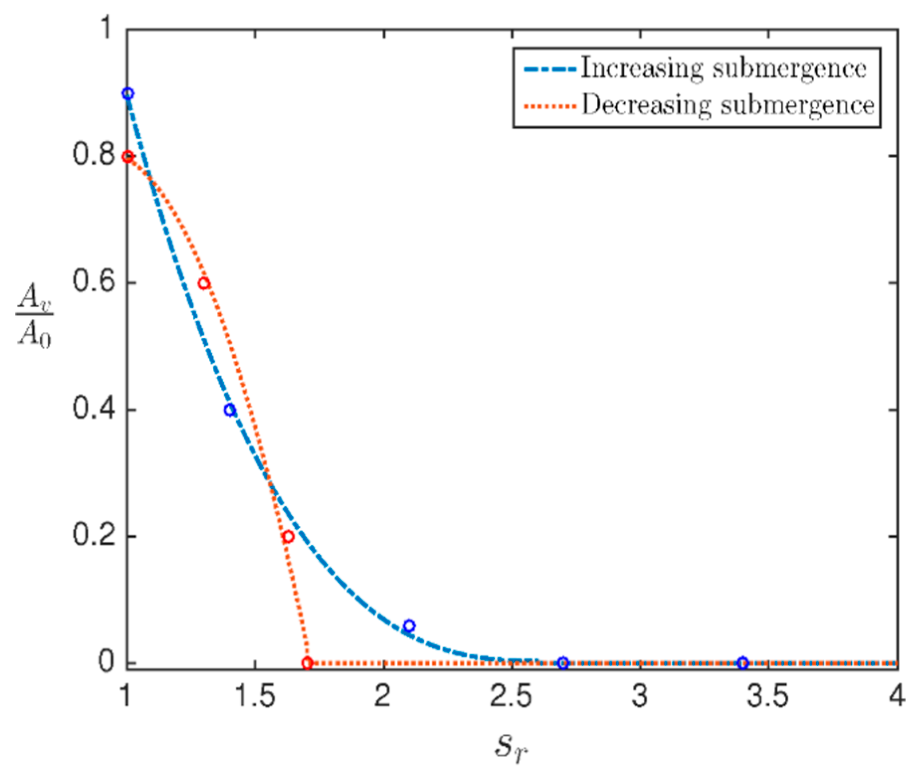
The main problem with using Equation (2) is to estimate the blade area that is covered by air . For bollard and low advance ratio conditions (J < 0.1), a polynomial relation between the ventilated blade area ratio and submergences developed by Dalheim and presented by Steen et al. [13] is used.
By using the steady state vortex ventilation model based on the vortex model from Rott [15] and the propeller momentum theory, it is possible to estimate due to vortex formation for advance numbers . The vortex model depends on two parameters: a source strength, which is related to the propeller loading, and the ambient vorticity; the sink gathers vorticity to form the vortex. The ambient vorticity in the towing tank is partly generated by the propeller wake and, therefore, again related to the propeller load through the circulation. A tuning constant is added to the calculation model in order to account for the effect that not all the propeller blade circulation is converted into ambient vorticity (0.6). The application of the vortex model from Rott [15] is described in Kozlowska et al. [8].
2.3. Thrust Loss due to Ventilation and Out-of-Water Effects
Free surface ventilation occurs for propeller submergences –1 < h/R < 1.2. The dominating thrust losses are, at least in most cases with significant forward speed, not due to ventilation but due to loss of submerged propeller disk area. We can separate the thrust losses as follows: thrust loss due to loss of propeller disc area, thrust loss due to wave making, thrust loss due to ventilation and due to the Wagner effect. For propeller submergence h/R < 1, the thrust has to be corrected for loss of propeller disc area.
The total thrust losses can be divided in loss of propeller disc area , Wagner effect, steady wave motion , and ventilation as follows:
Loss of propeller disc area for h/R < 1 can be estimated using purely geometrical considerations, as in Gutsche [10], as follows:
Dalheim [14], reproduced in Steen et al. [12], gave a more elaborate formula, where the influence of the hub is included, but the difference is not very significant, and the use of the above, much simpler formula is acceptable in most cases. The Wagner effect (Wagner, [9]) accounts for the dynamic lift effect. If the lift of a foil is changed suddenly by a sudden change in geometric angle of attack, the corresponding change in lift is first only half of the final steady value due to the induced angle of attack from the shed vortex formed by the time rate of change of circulation. This effect diminishes gradually, and a curve-fit formula is used in the equation below. It shows that the foil must travel about 20 chord lengths to almost recover full lift. The idea is that a similar effect occurs when a propeller blade is suddenly passing through the surface and into the water. The thrust loss factor is calculated from the average value during the submerged part of the blade rotation. Thus, it will, in general, depend on the propeller radius as well as propeller submergence. For the simplified formula, is modeled at the characteristic section . Therefore, the thrust loss factor due to the dynamic lift effect, which is relevant only for h/R < 1, is calculated as:
where is the local relative velocity at the blade section, which, when ignoring induced velocities, can be calculated as , t is propeller blade thickness, and c is the chord length.
Minsaas et al. [11] proposed an empirical expression for the combined effect of loss of disk area, wave making, and Wagner effect:
2.4. Torque Loss due to Ventilation and Out-of-Water Effects
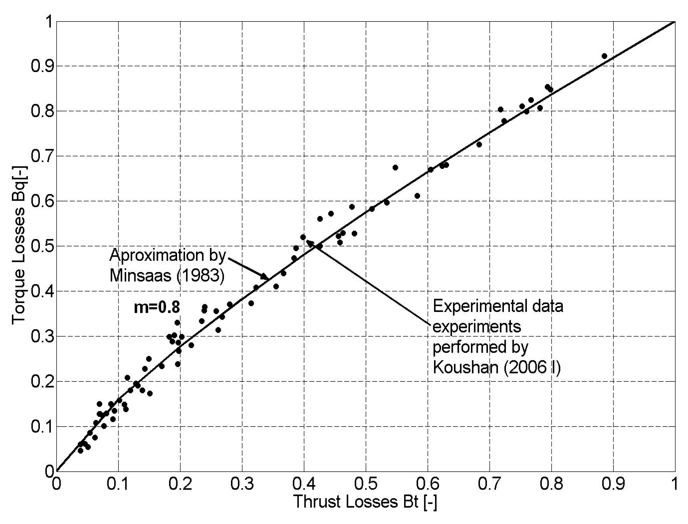
Figure 1 shows a relation between the torque loss factor and the thrust loss factor. As it is observed from Figure 1, the propeller torque has similar behavior as propeller thrust and shows good agreement with experimental results by Minsaas et al. [12],
where m is constant between 0.8 and 0.85 [13].
This means that if the torque is measured, one can also accurately know the thrust in ventilated conditions, and it means that when thrust loss is predicted or simulated, for instance, using the methods in this paper, the corresponding torque loss can easily be determined using Equations (9) and (10) with m = 0.8.
2.5. Time Domain Simulation Model: PropSim (2016) and PropSim (2018)
The propeller simulation model PropSim (2016) was developed by Dalheim [14] and implemented in Simulink. The simulation model generates a time domain solution to the six degrees of freedom propeller forces in varying operating conditions, including change of operating point, unsteady axial and tangential flow field, effect of oblique inflow in manoeuvring condition, Wagner effect, reduced propeller submergence, and ventilation. The time domain simulation model in PropSim (2016) is quasi-static. For ventilation modelling, PropSim (2016) used a formula based on an idea presented in Kozlowska and Steen [4], where the change in lift coefficient due to ventilation is used to compute the change in resulting in the formula for the thrust loss calculations due to ventilation presented in Equation (2).
For the PropSim (2016) simulation model, Dalheim used model tests from Kozlowska and Steen [4] to construct a polynomial relation for the value of the ventilated blade area ratio Figure 2 contains two different curves, one for increasing and one for decreasing propeller submergence, which indicate the propeller hysteresis behavior of the propeller ventilation.
The empirical relation presented in Figure 1 is used for the simulation model PropSim (2016) and can hardly be viewed as generally valid since other factors like forward speed and propeller loading must be expected to matter, Steen et al. [13]. Therefore, the simulation model (PropSim(2018)) has been updated by adding a physics-based model for estimating the ventilated area of the propeller disc based on propeller loading and submergence, outlined in Section 2.3 above. Like PropSim (2016), the simulation model PropSim (2018) is quasi static, since it is assuming that the response is quasi steady and based on the calculation model presented in Kozlowska et al. [8].
3. Results
3.1. Simulation Model Validation
Validation of the simulation model denoted PropSim (2018) is carried out using model experiments performed by Koushan [2] and Kozlowska et al. [8]. These two experimental campaigns are referred to in this article by using acronyms: experiments reported by Koushan [2]—Kou2006_I, and experiments reported by Kozlowska et al. [8]—Koz17.
Kou2006_I experiments were performed on an open pulling propeller exposed to forced sinusoidal heave motion. Carriage speed U and the propeller shaft frequency n were varied in order to obtain different low advance numbers J (around 0.1). In order to obtain more data for validation purposes in higher advance numbers, Koz17 experiments were performed. The testing conditions are listed in Table 1.
The same propeller model (P1374) was used for these experiments: the propeller has a diameter of 250 mm, design pitch ratio of 1.1, and expanded area ratio of 0.595. The propeller hub diameter is 65 mm.
The Kou2006_I experiments were conducted in the Marine Cybernetics Laboratories at the Norwegian University of Science and Technology. The tank is 40 m long, 6.45 m wide, and 1.5 m deep. Ventilation is generated by sinusoidal vertical motion of the propeller with different amplitudes. Blade axial, radial, tangential forces, and moments about all three axes were measured during the experiments. A pulse meter indicating the angular position of the reference blade.
The Koz17 experiments took place in the large towing tank at SINTEF Ocean in Trondheim, with dimensions (length × breadth × depth) of 260 m × 10.5 m × 5.6 m. The tests were performed at different submergence ratios and propeller rotational speeds. For each draught and propeller rotational speed, the propeller was tested at different advance numbers ranging from to . Different advance numbers were obtained at various propeller rotational speeds so that for the same advance numbers, different propeller thrusts were obtained, thus varying the Weber number . A conventional two components propeller open water dynamometer was used to measure propeller thrust and torque. The main purpose for these experiments was to obtain more data at higher advance numbers. Also, the different advance numbers were obtained at a range of propeller rotational speeds that, for the same advance number, different thrust coefficients were tested.
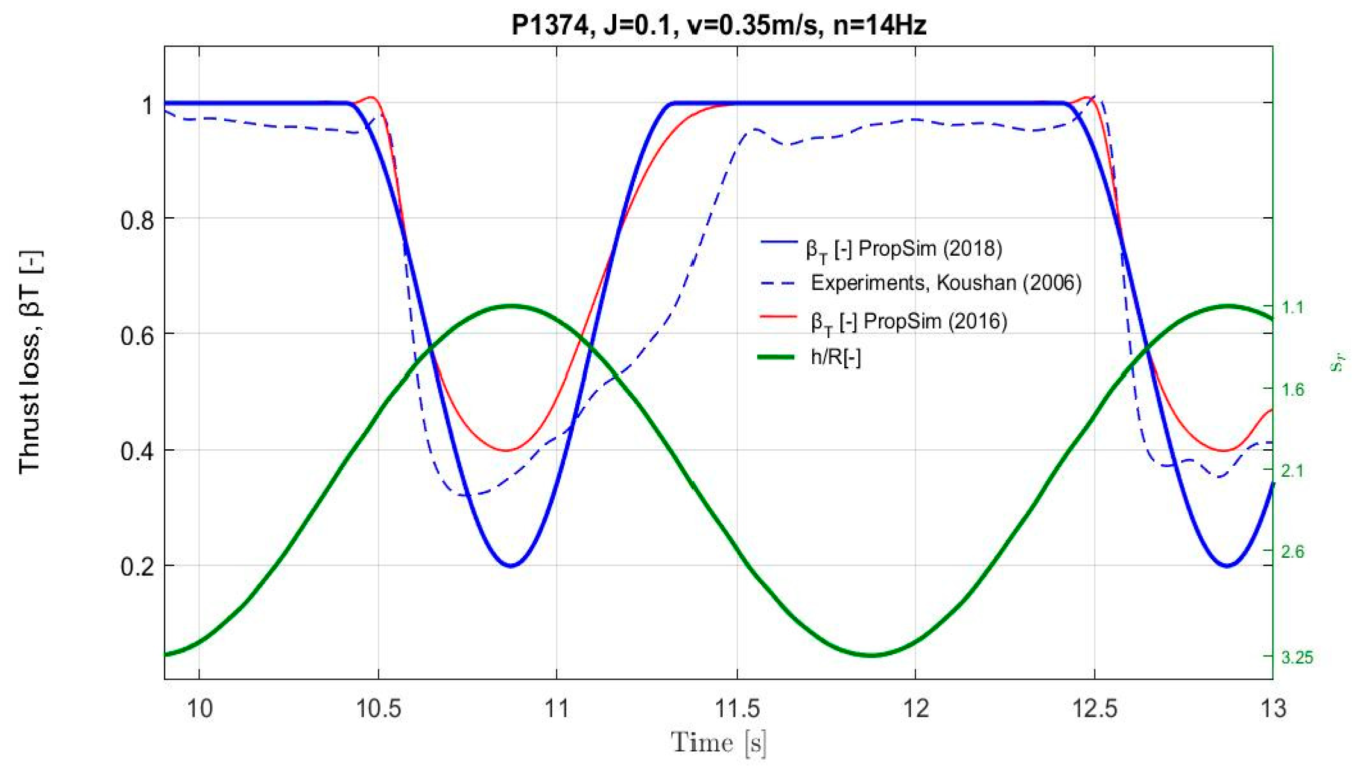
Figure 3 shows the comparison between a simulation performed by using PropSim (2016) and PropSim (2018) simulation models and experimental results, Kou2006_I. PropSim (2016) model relates thrust loss to the estimated ventilated blade area using an empirical relation that is based on the same model experiments, as shown in Figure 3 (Kou2006_I). This is believed to be the reason why, for this particular case, the agreement between experimental results and calculation fitted better to the 2016 version of the simulation model.
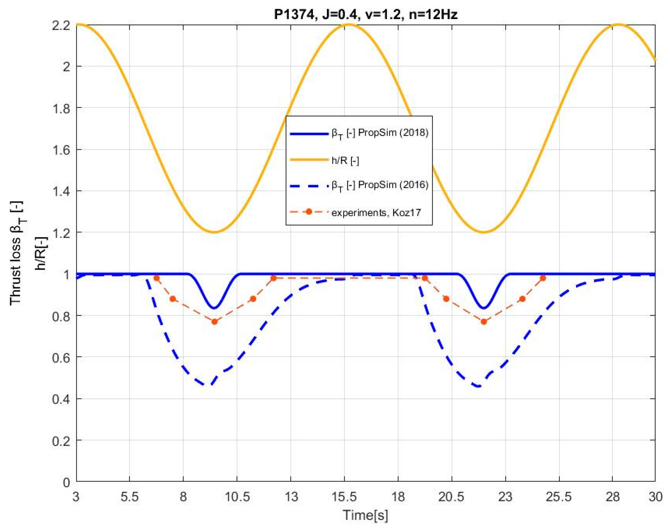
Figure 4 shows the comparison of thrust loss calculations using two different versions of the simulation model: PropSim (2016) and PropSim (2018). Propeller thrust loss is calculated for a propeller working at constant propeller revolutions n = 12 Hz under dynamic heave motion conditions for high advance number J = 0.4. There are no experimental conditions testing propeller ventilation during dynamic heave motion for high advance numbers, thus for validation purposes, the simulation model results have to be compared with static conditions based on the Koz17 experiments, implicitly assuming that the behavior is quasi-static. It can be observed from Figure 4 that the thrust loss prediction agrees better with the calculations performed by using the simulation model PropSim (2018). The reason for this result is that the simulation model PropSim(2016) does not include the forward speed and propeller loading as a factor for calculating the blade area ratio . Simulation model PropSim (2016) overestimated thrust losses due to ventilation. For example, for h/R = 1.2, the thrust loss due to ventilation is 0.84 based on the PropSim (2018) simulation model and in the range of 0.45–0.5 for the PropSim (2016) simulation model. The experimental measurements are equal to 0.78, which is closer to the updated simulation model PropSim (2018). The same behavior was observed for other submergence ratios h/R = 1.4, 1.6, and 2.0.
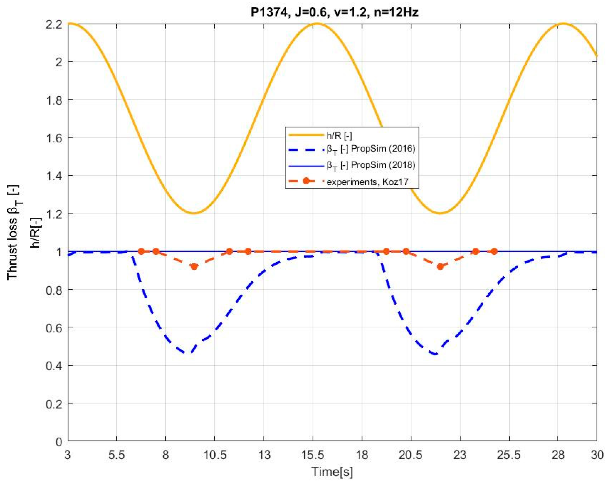
Figure 5 shows the comparison of thrust loss calculation using the PropSim (2016) and PropSim (2018) simulation model. Propeller thrust loss is calculated for the propeller working with constant propeller revolutions n = 12 Hz under dynamic heave motion conditions for the high advance number J = 0.6. It can be observed from Figure 5 that the thrust loss prediction agrees better with the calculation for the simulation model PropSim (2018). Simulation model PropSim (2016) overestimates thrust losses due to ventilation. For example, for h/R = 1.2, the thrust loss due to ventilation is 1.0 based on the PropSim (2018) simulation model and is in the range of 0.45–0.5 for the PropSim (2016) simulation model. The experimental measurements are equal to 0.92, which is closer to the updated simulation model PropSim (2018). Also, experimental data based on experiments Koz17 shows no thrust loss for J = 0.6 for the submergence ratio the same as predicted by using the PropSim (2018) simulation model.
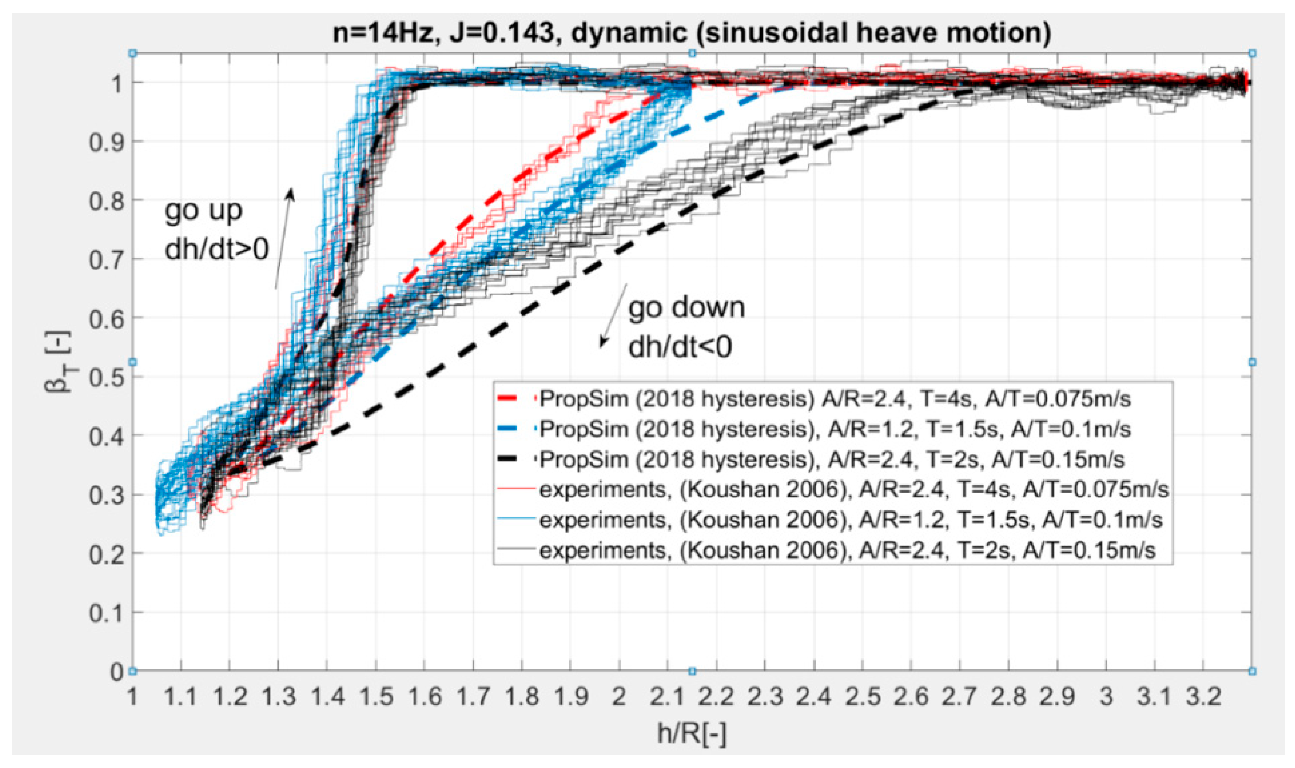
3.2. Dynamic Effect Causing Hysteresis of the Thrust Loss during Heave Motion of the Propeller Calculated by PropSim (2018_hysteresis)
A significant dynamic effect of propeller ventilation is connected with the thrust and torque hysteresis effect, appearing mostly in connection with intermittent vortex ventilation. The hysteresis effect is caused by the fact that it takes a while for ventilation of a submerged propeller to be established, so in a situation with decreasing submergence or increasing propeller loading, there is less thrust loss than for the same condition in static operation, while when ventilation disappears, it takes time for the thrust to build up, due to the Wagner effect, so then thrust loss is larger than the corresponding static operation.
In order to account for this effect, the PropSim (2018) simulation model was updated. The dynamic effect was added by making propeller circulation, described in Equation (11) as a time dependent function.
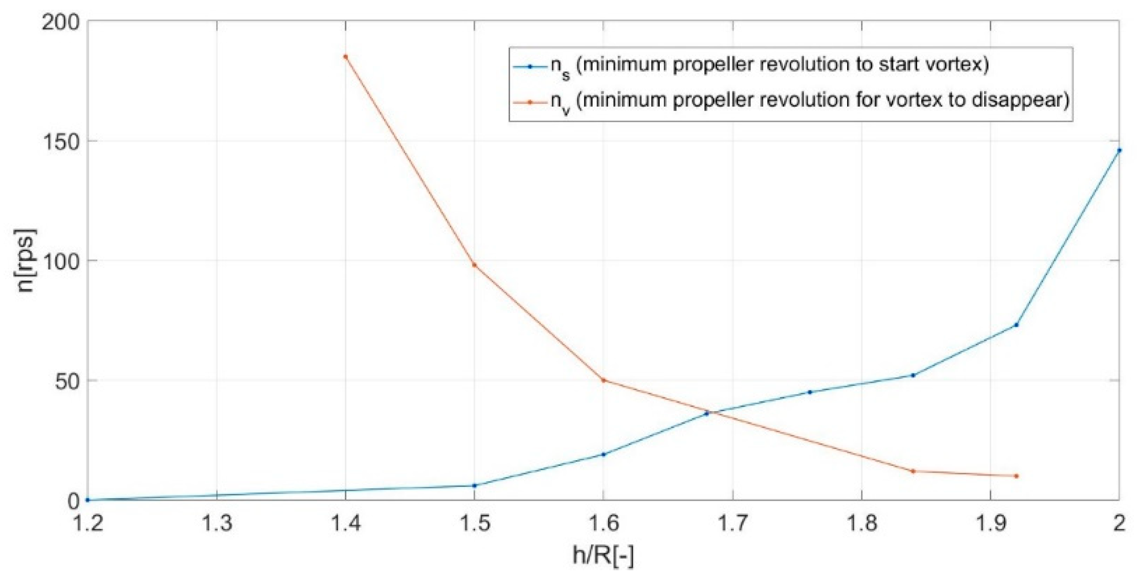
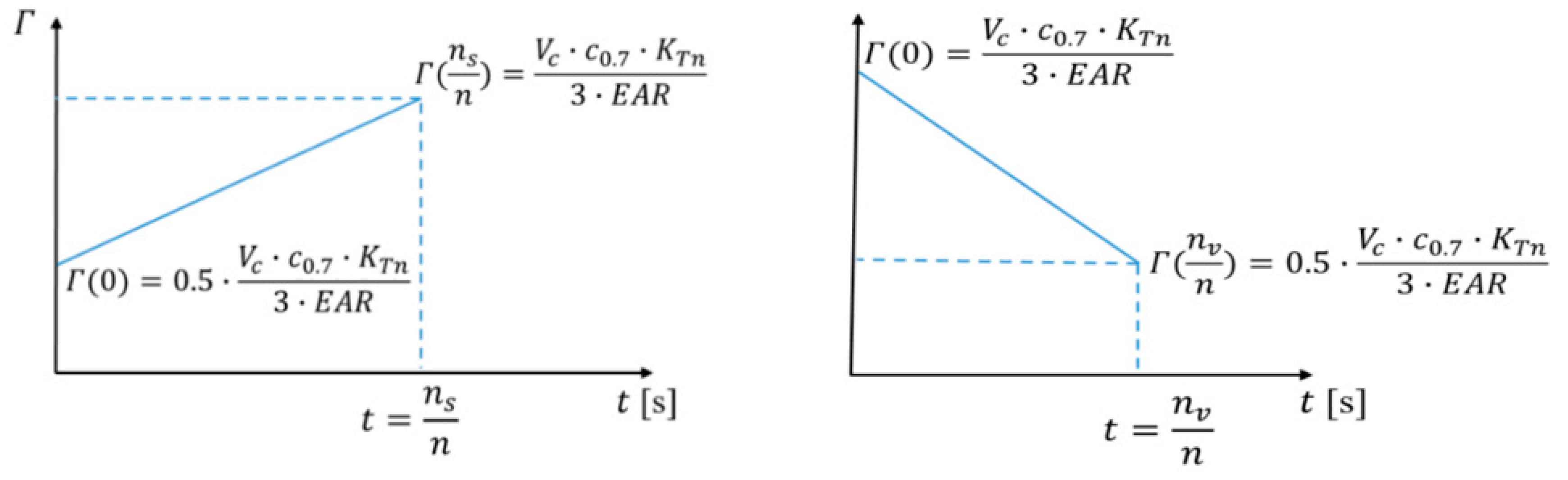
The time dependent function was divided into two different cases. One, which corresponds with time, which is required to establish ventilation, and the other, which corresponds with time, which is desired for ventilation to disappear. Symbol , which is used in Figure 6, is the minimum number of propeller revolutions needed to establish ventilation, thus forming a ventilating vortex from the free surface, and symbol used in Figure 6 is the minimum number of propeller revolutions needed for a vortex, and thereby ventilation to disappear. and are functions of propeller submergence for low advance numbers . Higher advance numbers are not covered since, then, vortex ventilation is found to be very unlikely, and for free surface ventilation, little or no hysteresis effect is observed in experiments. Propeller circulation as a function of time for the creation and disappearance of vortex ventilation is presented in Figure 7. Since in principle vortex ventilation is dependent on the surface tension, while the proposed model does not include any effect from surface tension, the model presented here is only valid for high Weber numbers, taken to be . Polynomial approximations of and are presented in the equations below.
Table 2 shows five different experimental conditions that were used for the comparison between calculations using the PropSim (2018 hysteresis) simulation model and experimental results. A is the amplitude of the harmonic heave motion, while T is the period of the harmonic heave motion.
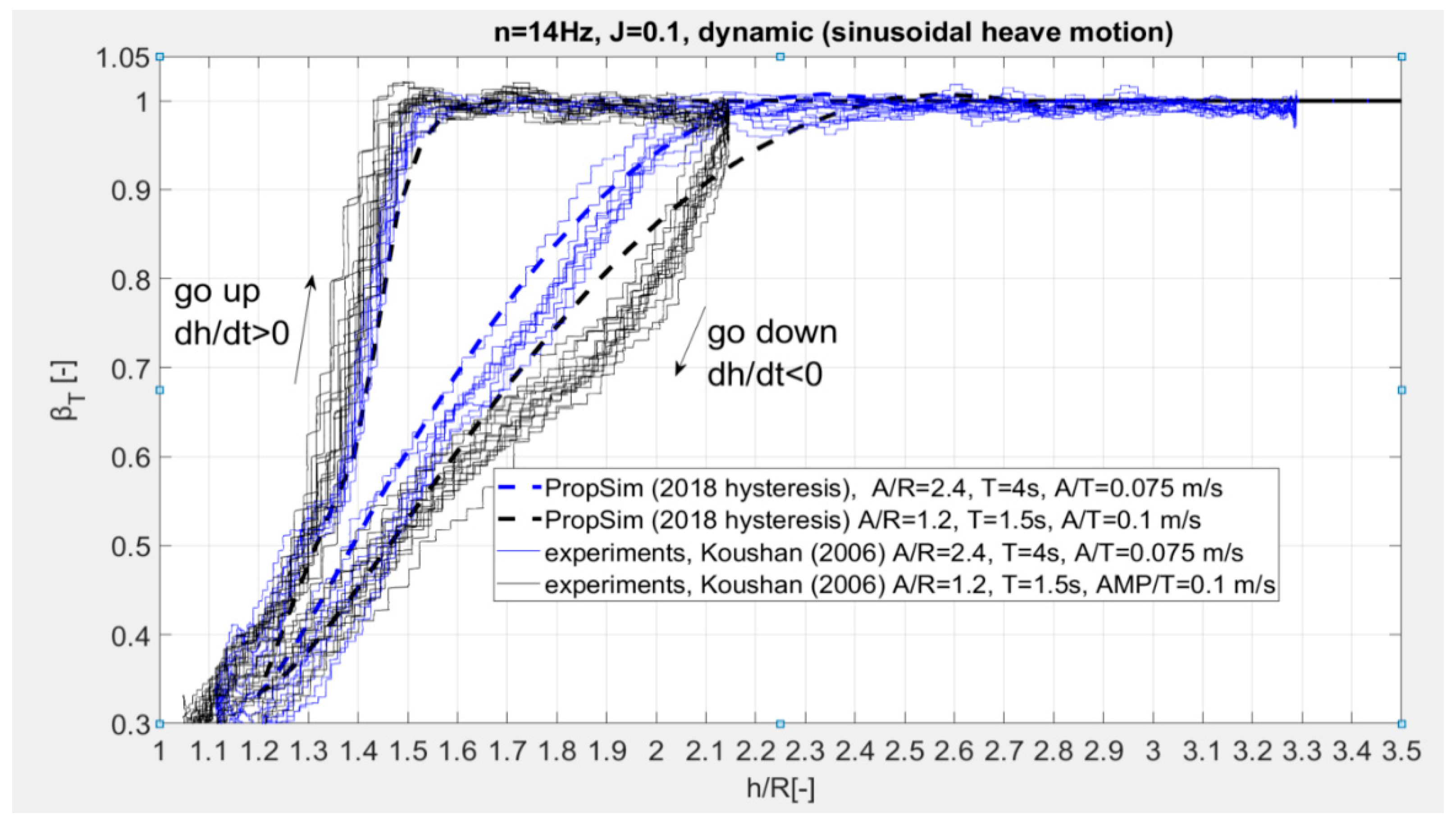
Figure 8 and Figure 9 show the comparison of thrust loss in the experiments under dynamic heave motion for different heave amplitudes and calculations by using the simulation model PropSim (2018_hysteresis), which includes the hysteresis effect in the simulation. As can be observed in the figures, calculations performed by the PropSim (2018_hysteresis) simulation model agree quite well with experiments. This means that the simulation model correctly accounts for the hysteresis effect on ventilation due to the propeller working with periodically varying submersions.
3.3. Dynamic Effect, Thrust Loss due to Ventilation as a Function of Blade Position Calculated by PropSim (2018_blade_dynamics)
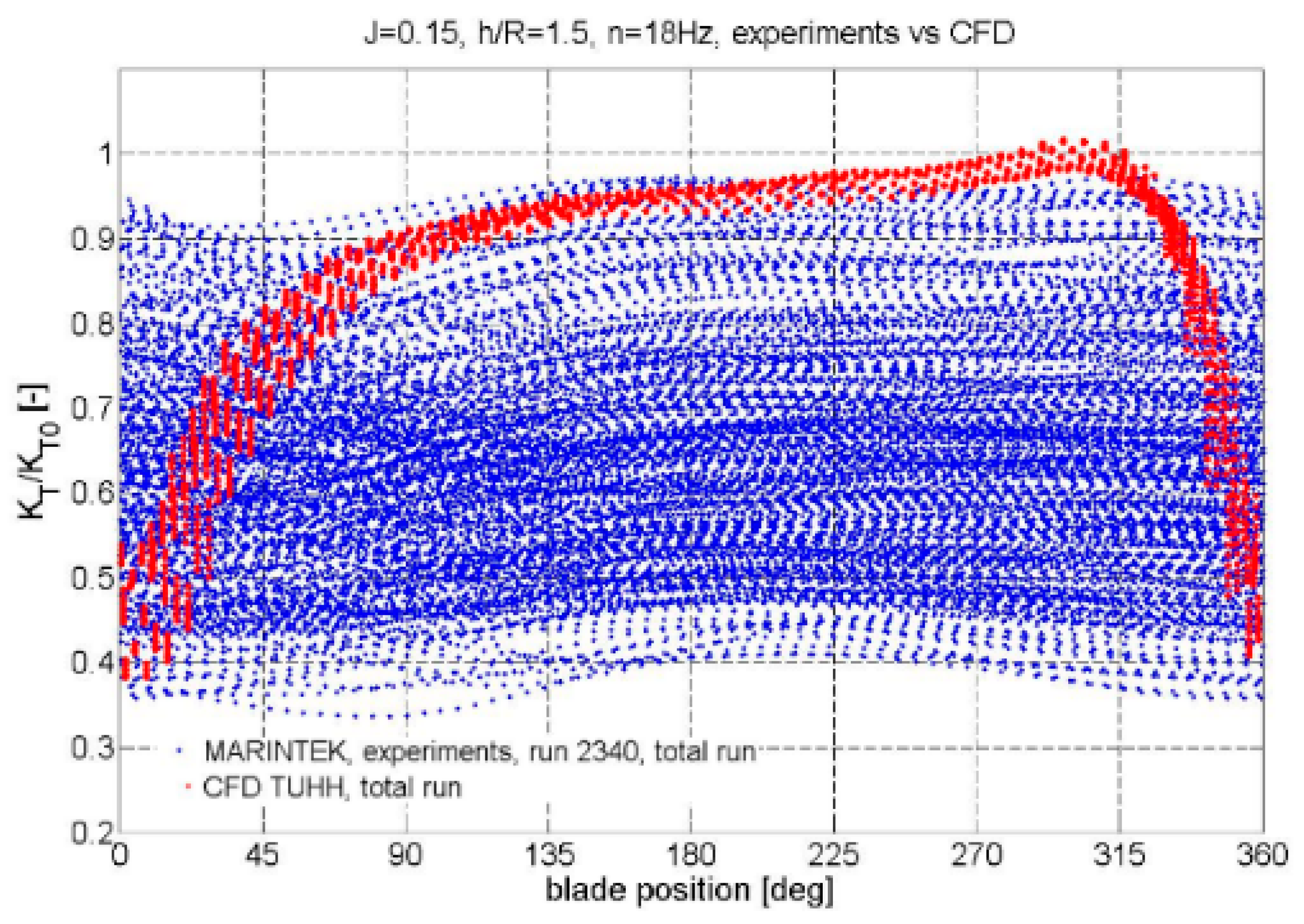
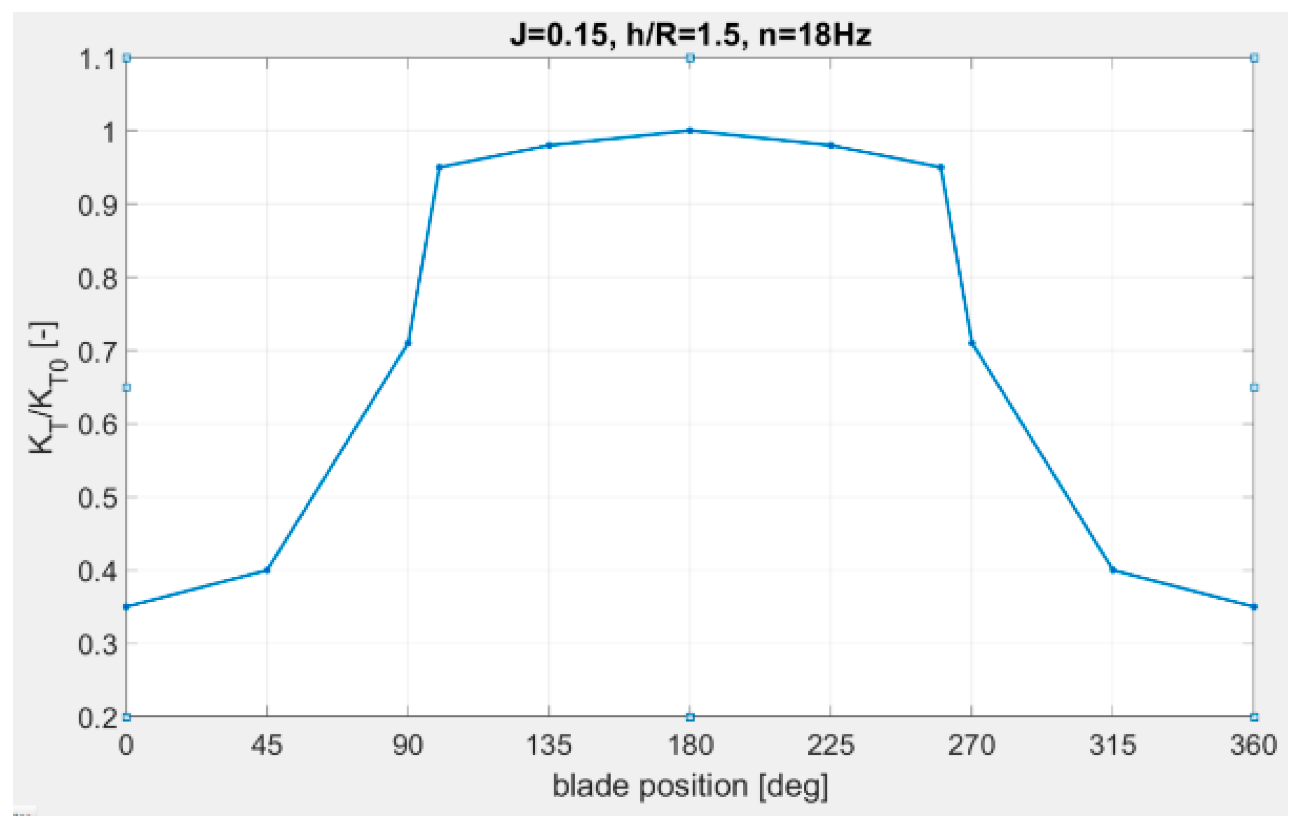
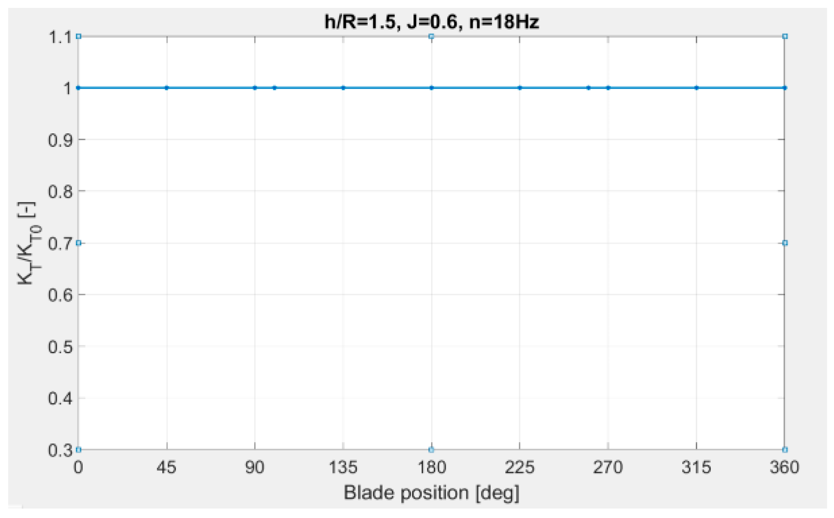
From the experiments, it can be observed that the thrust varies with the position of the blade during one cycle of rotation when the propeller is ventilating and/or coming partly out of water. For deep and constant propeller submergence and low advance numbers (i.e., h/R = 1.5 and J = 0.15, no out of water effect), the biggest thrust loss is found when the blade is close to the free surface (between and ). For the propeller blade position between and , the thrust is rebuilt and achieves values close to the nominal thrust. The different thrust losses correspond to the different ventilation extent. It is clear from the experiments that in this condition the propeller blade can be both fully, partially, or non-ventilating depending on the blade position. When the propeller is coming out of the water (i.e., h/R = 0), the thrust loss also varies due to the blade position. The three reasons for this variation are ventilation, loss of propeller disk area, and Wagner effect. The previous versions of the simulation model denoted PropSim (2016) and PropSim (2018) both include the loss of propeller disk area and the Wagner effect as a function of propeller position. In the previously described versions of PropSim (2018), the thrust averaged over a propeller revolution is calculated, meaning that propeller blade frequency dynamics are not represented in the simulation, see Figure 10a. In order to include blade frequency dynamics, the blade thrust is computed as a function of the blade position, see Figure 10b.
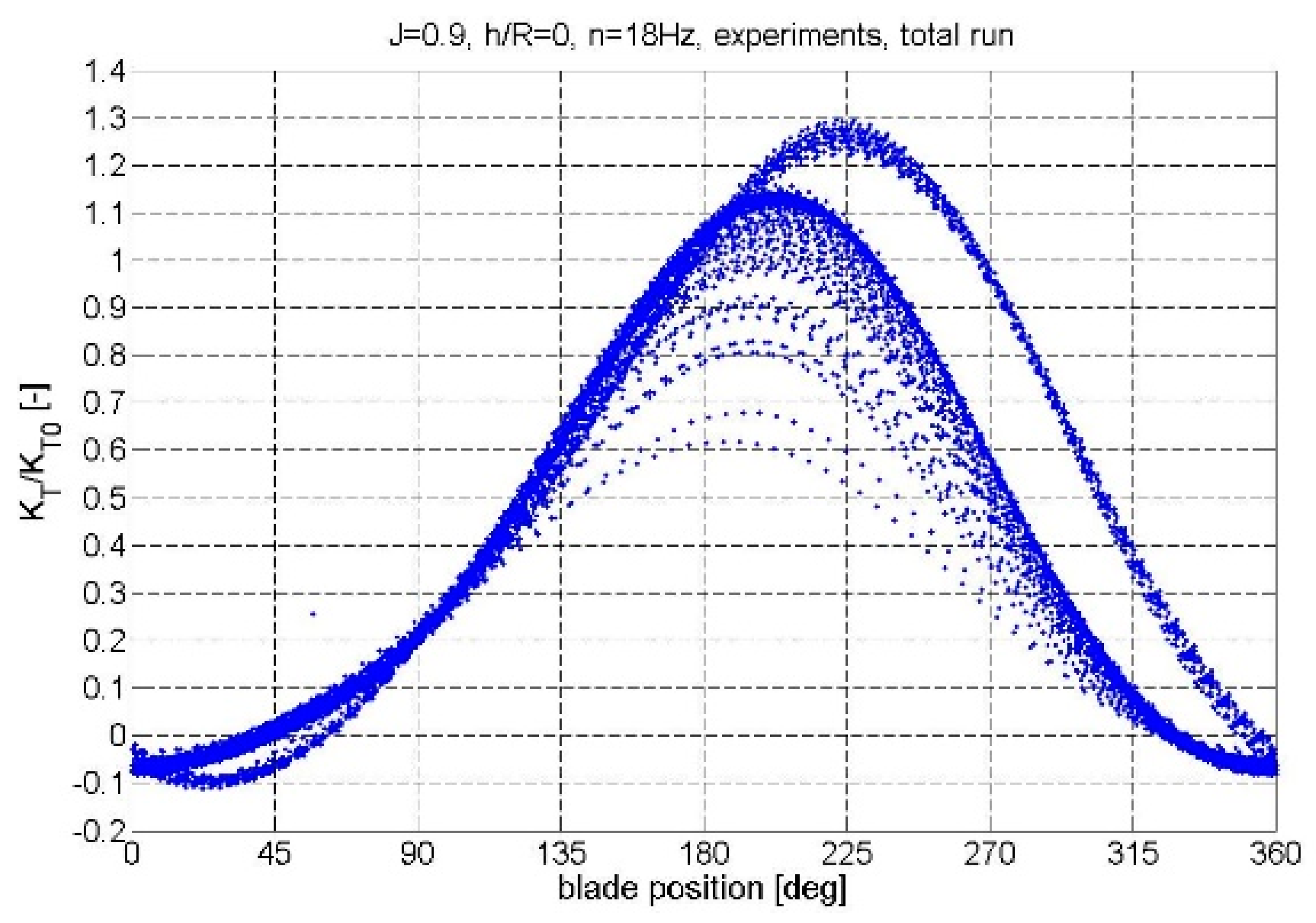
Figure 11 shows the comparison between calculations (CFD) and experiments Koz10 of the thrust loss due to ventilation as a function of blade position. The CFD calculations were performed by TUHH (Hamburg University of Technology) and based on their in-house code FreSco+. The method used in the calculation was a RANS (Reynolds Averaged Navier Stokes) code based on a finite volume discretisation of the computational domain. For the investigation presented below, the propeller is modelled in the cylindrical domain, which rotates with the number of revolutions of the propeller; see Wockner-Kluwe [16]. It can be observed from the figure that the prediction of thrust loss is more repeatable between revolutions for CFD calculations than for experiments. Figure 12 shows the calculation of the thrust loss due to ventilation, which varies due to different blade positions (PropSim (2018_blade_dynamics)).
It can be observed from the comparison of Figure 11 and Figure 12 that the calculations made by simulation using PropSim (2018_blade_dynamics) are closer to the CFD computational results than the experimental results. For both CFD and simulations, similar thrust loss is observed for every propeller revolution. During measurements, different thrust losses appear depending on the time in the experiments, see Figure 11. The reason for the large variation of thrust loss between the propeller revolutions is not known. Measurement error is unlikely, given the repeatability of measurements in fully-submerged conditions in the same experimental campaign. It is believed that the variation might be caused by the ventilatilon in this condition being unstable and on the limit between the ventilated and non-ventilated condition. When the propeller ventilates, the thrust is reduced, so the thrust loading is reduced, and thereby reducing the ventilation probability, which, in turn, causes the ventilation to disappear after some time. The fact that it takes some time for the ventilation to disappear is what causes the hysteresis effect discussed earlier. When the ventilation disappears, the thrust and, therefore, thrust loading increases again, leading eventually to new ventilation. The reason for the perfectly symmetric appearance of the thrust loss factor versus the blade angle in Figure 12 is that the calculation method is quasi-static—it does not capture the “memory effect” of the flow, which is present in both reality and CFD.
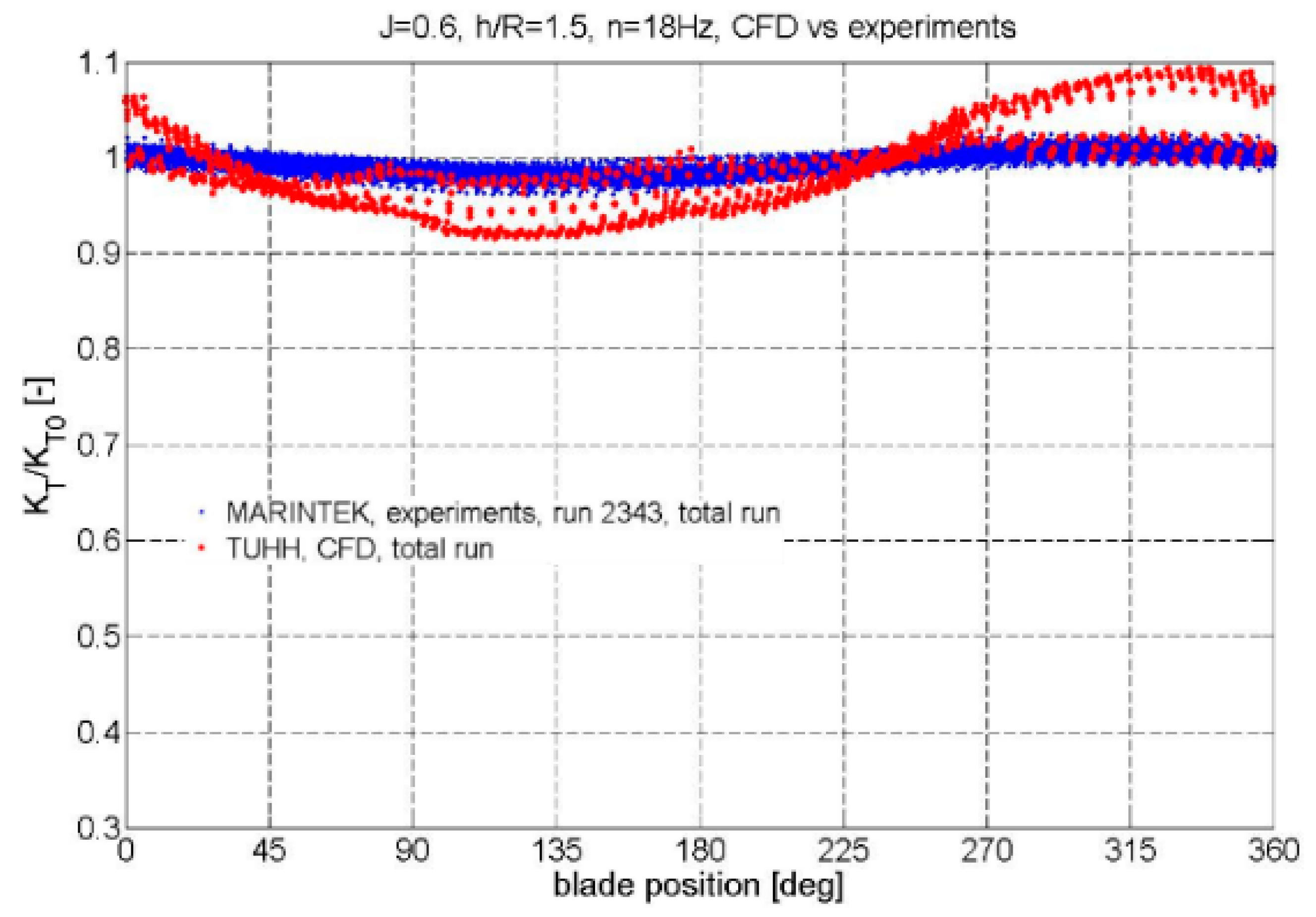
Figure 13 and Figure 14 show the thrust loss variations at different blade positions for n = 18 Hz and higher advance numbers. Figure 13 shows the comparison between calculations (CFD) and experiments Koz10 of the thrust loss due to ventilation as a function of blade position. Figure 14 shows the calculation of the thrust loss by using the PropSim (2018_blade_dynamics) simulation model. By comparing the two figures, it is seen that both experiments and PropSim-calculations show hardly any thrust loss. For the experiments, there is a very slight variation of thrust, which is not due to ventilation but might be caused by the free surface (wave making) effect. For PropSim, this type of free surface effect is not modeled. The CFD shows a thrust that varies with position, although showing a partly higher thrust than the nominal. The reason for this variation is not known but might also be due to the free surface (wave making) effect.
- h/R = 1.5, n = 18 Hz, J = 0.6 (high advance number)
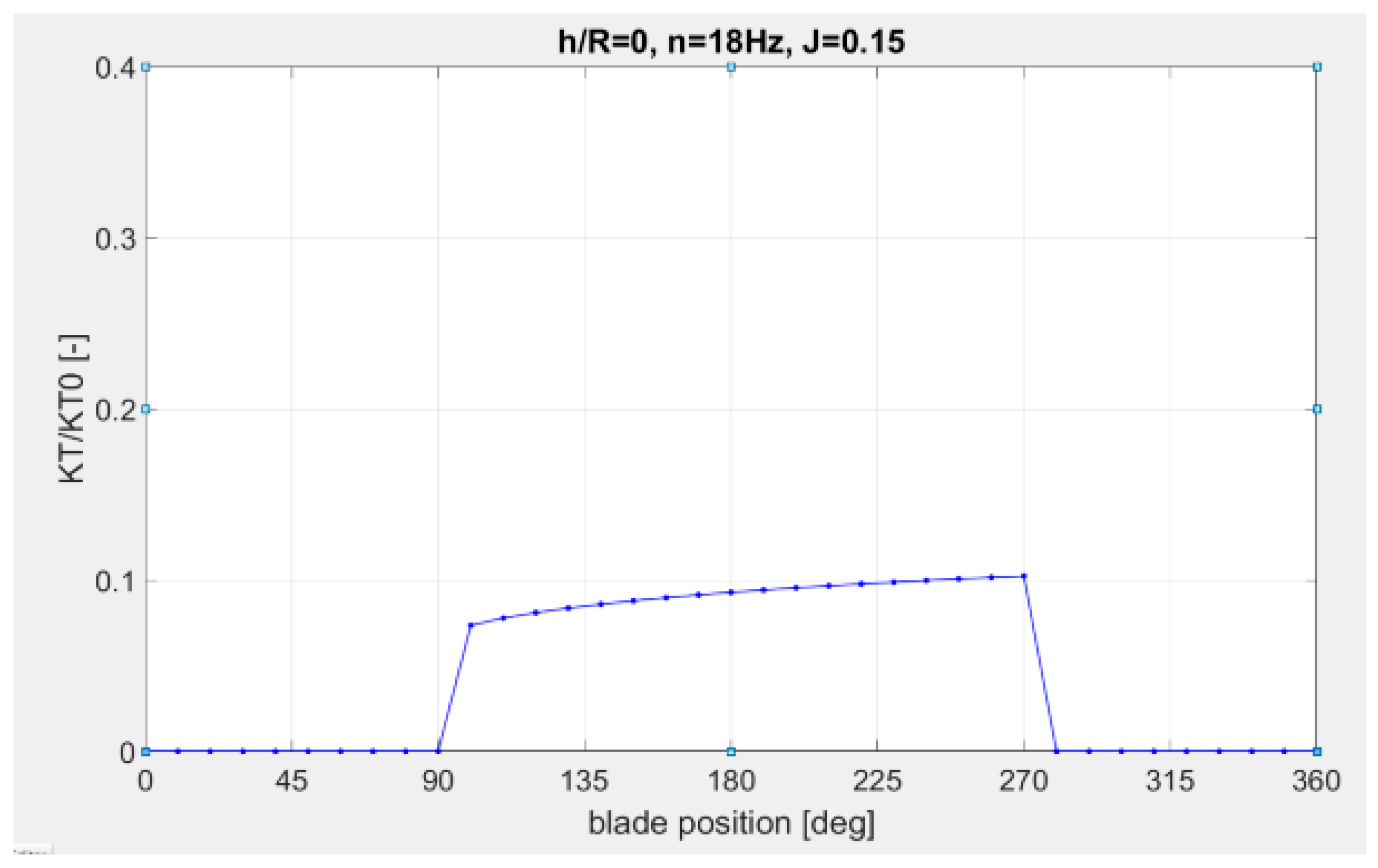
Figure 15 and Figure 16 show the thrust variations at different blade positions in one cycle of revolution for n = 18 Hz and a low advance number. For this case, the propeller is half submerged, so different thrust loss is a consequence of a combination of the out-of-water effect, Wagner effect, and ventilation. Figure 15 and Figure 16 show relatively good agreement between the experimental results and calculations, although the experimental results are more gradually changing compared to the simulation. The reason for this is because in the proposed method, the propeller blade forces are considered at the lifting line. This means that a half-submerged propeller will get zero propeller blade forces in the upper half of one revolution, as seen in Figure 16, which is inconsistent with the gradual variation seen from the experimental results in Figure 15. In the experimental results, the thrust has a peak of around 170°–180°; however, the thrust continues to increase until the lifting line leaves the water. This is due to the included Wagner effect, which gives a gradual increase in the thrust loss factor towards unity as the blade section travels up to around six chord lengths.
- h/R = 0 (half submerged), n = 18 Hz, J = 0.15 (low advance number)
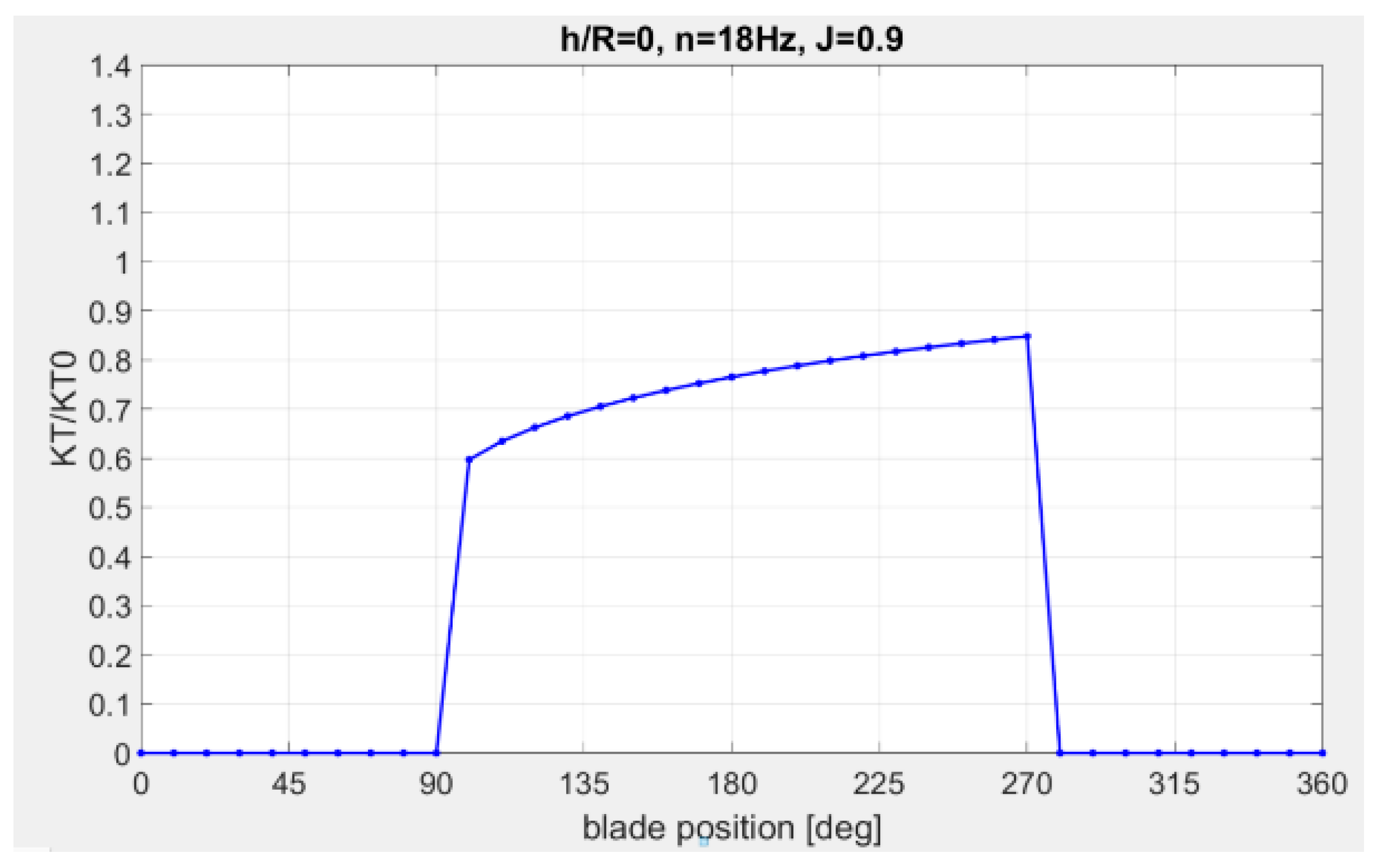
Figure 17 and Figure 18 show the thrust variations at different blade positions in one cycle of revolution for n = 18 Hz and a high advance number J = 0.9. For these cases, the propeller is half submerged, so a different thrust loss is a consequence of a combination of the out-of-water effect, Wagner effect, and ventilation. Figure 17 and Figure 18 show similar agreement for a high advance number as for a low advance number. In the experimental results, the thrust has a peak around 200°, i.e., after the blade has passed its lowest position. This can be explained by air dragged down by the propeller blade, causing loss of effective propeller blade area, which means that it will take a longer time for the thrust to build. In the proposed method, however, the thrust continues to increase until the lifting line leaves the water. Similar to a low advance number, this is due to the included Wagner effect. The thrust loss caused by air dragged down by the propeller blade does not vary along one revolution in the proposed method because it is calculated based on propeller submergence, not blade submergence. This is why a similar displacement of the thrust (relative to the bottom blade position) is not visible in the proposed method. The integrated value of thrust will, however, have its center around 200° in the proposed method, similar to the experimental results.
- h/R = 0 (half submerged), n = 18 Hz, J = 0.9 (high advance number)
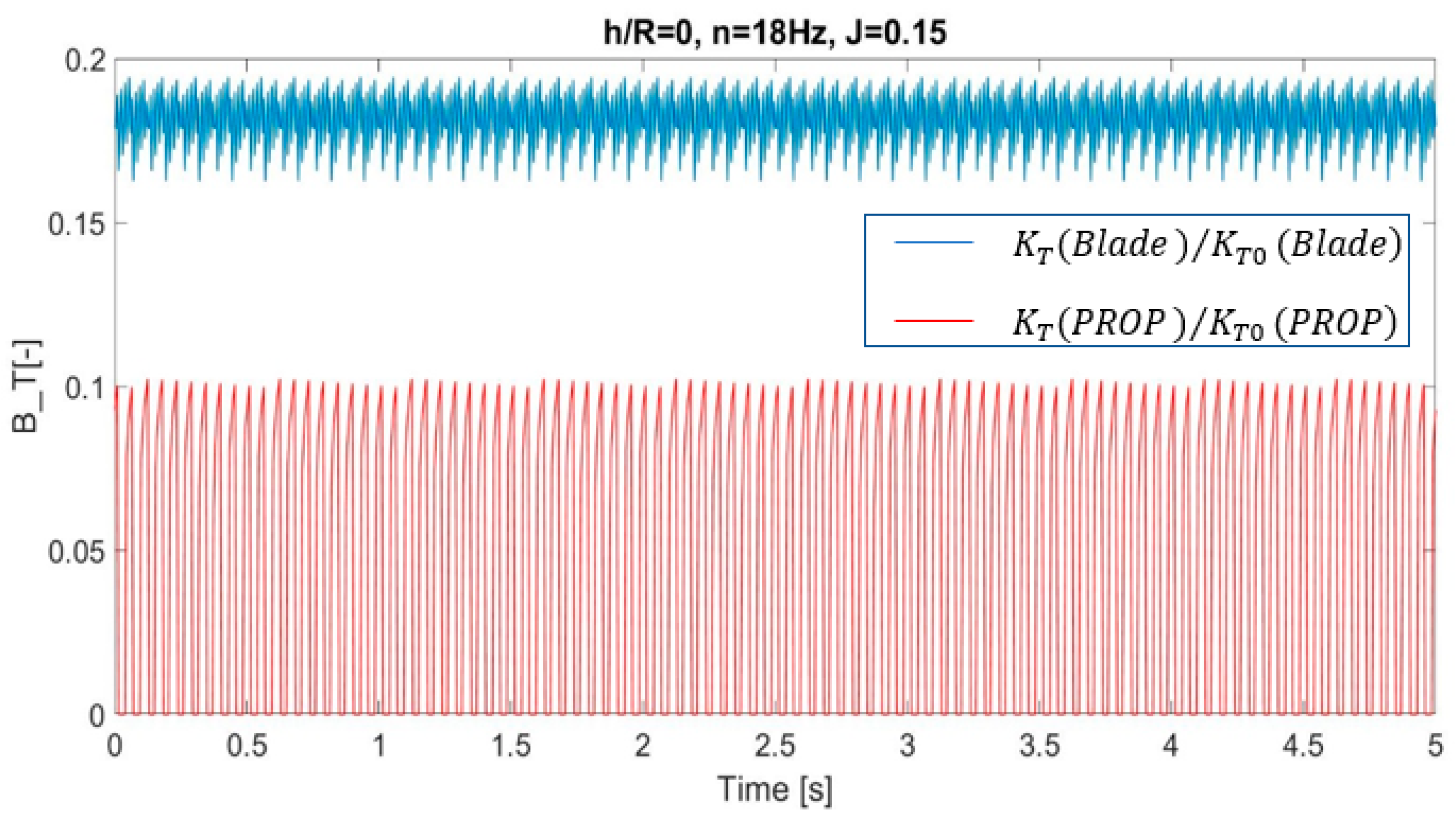
Figure 19 shows a time series of the computed thrust coefficient for a single blade and the propeller for J = 0.15, h/R = 0, n = 18 Hz made using the PropSim (2018_blade_dynamics) simulation model.
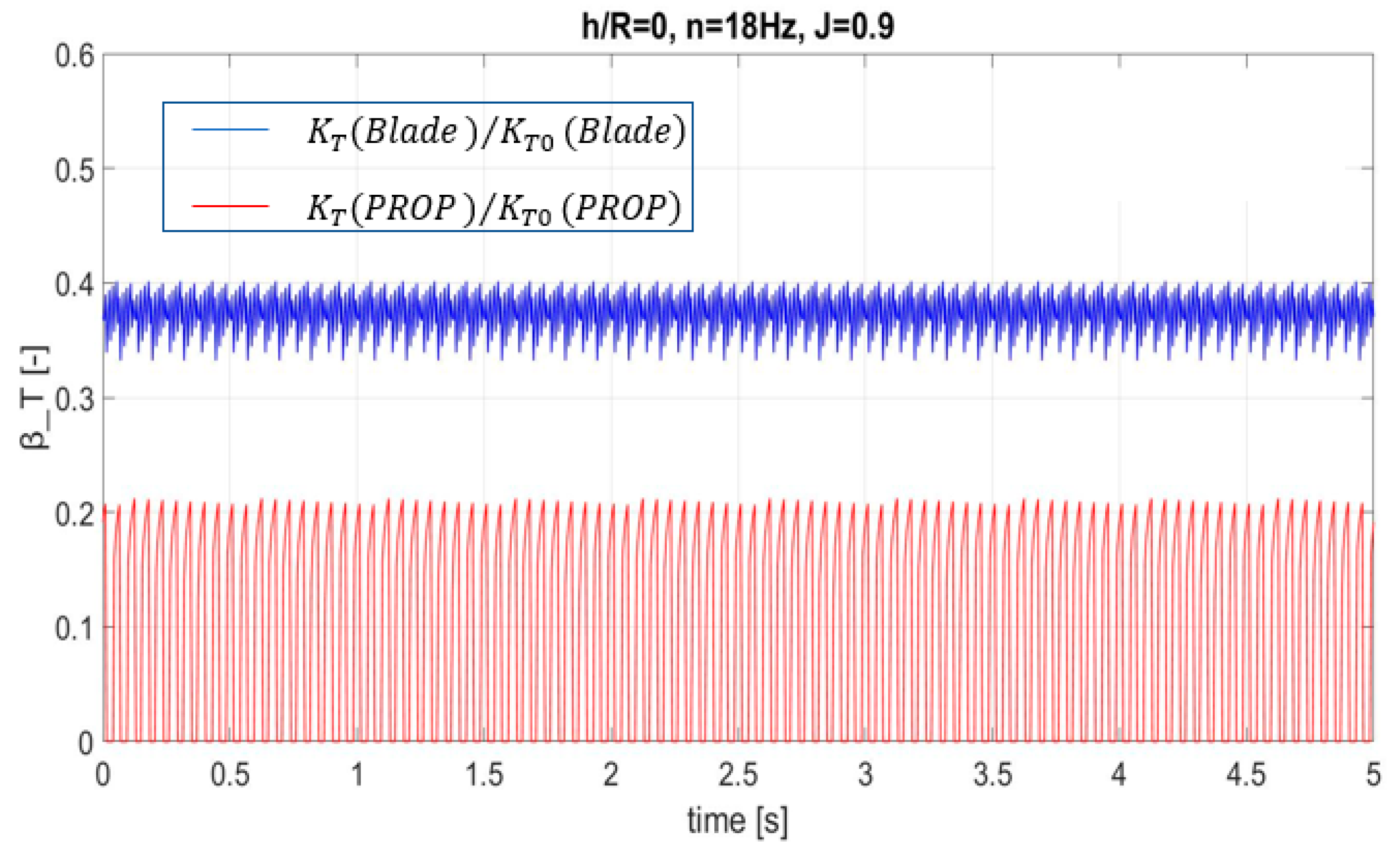
Figure 20 shows a time series of the computed thrust coefficient for a single blade and the propeller for J = 0.9, h/R = 0, n = 18 Hz made using the PropSim (2018_blade_dynamics) simulation model. Figure 19 is presenting results from the same computation as Figure 16, while Figure 20 is presenting results from the same computation as Figure 18. However, in Figure 19 and Figure 20, thrust loss is presented as function of time instead of angular position. Note also that while Figure 16 and Figure 18 use a thrust loss factor dividing the actual blade thrust with the nominal (non-ventilated) blade thrust, Figure 19 and Figure 20 are using a factor where the actual thrust is divided with the total propeller thrust.
4. Discussion and Conclusions
This paper presents a simple time-domain simulation model for thrust loss due to ventilation and the out-of-water effect. The thrust loss model can be used also for predicting torque loss, through a simple, empirical relation between thrust and torque loss. The presented simulation model is an extension of the model previously presented by Kozlowska et al. [8] and Dalheim [14].
Two different dynamic effects of the ventilating vortex have been added. One effect is connected with the dynamic effect causing hysteresis and connected with the propeller loading. The other dynamic effect is connected to the thrust loss variation with the position of the blade during one propeller revolution.
A significant dynamic effect of the propeller ventilation is connected with the thrust and torque hysteresis effect, appearing mostly in connection with intermittent vortex ventilation. The hysteresis effect is caused by the fact that it takes a while for the ventilation of a submerged propeller to be established, so in a situation with decreasing submergence or increasing propeller loading, there is less thrust loss than for the same condition in static operation. Also, when ventilation starts to disappear, it takes time for thrust to build up again, so that the thrust loss is larger than in the corresponding static operation. In order to account for this effect, the PropSim (2018) simulation model was further developed. The dynamic effect was added by including the time dependency of the propeller circulation in the calculation of propeller ventilation. The comparison between the simulation model PropSim (2018_hysteresis) and model experiments shows good agreement, which means that the simulation model correctly accounts for the hysteresis effect on ventilation due to propeller working with periodically varying submersion.
The other dynamic effect, which is connected to the blade position during one cycle of rotation, has been added to the simulation model denoted PropSim (2018_blade_dynamics). The comparison between the results obtained by the simulation model, experiments and CFD calculations shows that the simulation model is closer to the CFD computational results than the experimental results. For both CFD and simulation results, similar thrust loss was observed for every propeller revolution. During the experiments, different thrust losses depending on the time in the experiments were observed.
Author Contributions
Conceptualization, L.S., A.M.K. and Ø.Ø.D.; Data curation, A.M.K.; Formal analysis, A.M.K.; Investigation, A.M.K.; Methodology, A.M.K. and S.S.; Supervision, S.S.; Writing–original draft, A.M.K. All authors have read and agreed to the published version of the manuscript.
Funding
This research was founded by Kongsberg Maritime AS, NTNU and SINTEF Ocean.
Acknowledgments
This work has been carried out at the University Technology Centre at NTNU (Trondheim) sponsored by Rolls Royce Marine (now Kongsberg Maritime AS) and SINTEF Ocean.
Conflicts of Interest
The authors declare no conflict of interest.
References
- Califano, A. Dynamics Loads on Marine Propellers Due to Intermittent Ventilation. Ph.D. Thesis, Norwegian University of Science and Technology, Trondheim, Norway, 2010. [Google Scholar]
- Koushan, K. Dynamics of ventilated propeller blade loading on thrusters. In Proceedings of the World Maritime Technology Conference (WMTC), Rome, Italy, 17–22 September 2006. [Google Scholar]
- Kozlowska, A.; Steen, S.; Koushan, K. Classification of different type of propeller ventilation and ventilation inception mechanisms. In Proceedings of the First International Symposium on Marine Propulsors, smp09, Trondheim, Norway, 9 June 2009. [Google Scholar]
- Kozlowska, A.; Steen, S. Ducted and Open Propeller Subjected to Intermittent Ventilation. In Proceedings of the Eighteen International Conference on Hydrodynamics in Ship Design, Safety and Operation, Gdansk, Poland, 12–13 May 2010. [Google Scholar]
- Smogeli, Ø.N. Control of Marine Propellers: From Normal to Extreme Conditions. Ph.D. Thesis, Norwegian University of Science and Technology, Faculty of Engineering Service and Technology, Department of Marine Technology, Trondheim, Norway, 2006. [Google Scholar]
- Koushan, K. Dynamics of Ventilated Propeller Blade Loading on Thruster due to Forced Sinusoidal Heave Motion. In Proceedings of the 26th Symposium on Naval Hydrodynamics, Rome, Italy, 17–22 September 2006. [Google Scholar]
- Koushan, K. Dynamics of Propeller Blade and Duct Loading on Ventilated Ducted Thruster Operating at Zero Speed. In Proceedings of the International Conference on Technological Advances in Podded Propulsion, Brest, France, 3–5 October 2006. [Google Scholar]
- Kozlowska, A.; Savio, L.; Steen, S. Predicting Thrust loss of ship propellers due to ventilation and out of water effect. J. Ship Res. 2017, 61, 198–213. [Google Scholar] [CrossRef]
- Wagner, H. Über Stoß- und Gleitvorgänge an der Oberfläche von Flüssigkeiten. Z. Angew. Math. Mech. 1932, 12, 192–235. [Google Scholar] [CrossRef]
- Gutsche, F. Der Einfluss der Kavitation auf die Profileigenschaften von Propellerblattschnitten, Schiffbauforschung, Heft 1; Wasserbau und Schiffbau: Berlin, Germany, 1962. [Google Scholar]
- Faltinsen, O.; Minsaas, K.; Liapas, N.; Skjørdal, S.O. Prediction of Resistance and Propulsion of a Ship in a Seaway; The Shipbuilding Research Association Japan: Tokyo, Japan, 1981. [Google Scholar]
- Minsaas, K.; Faltinsen, O.; Person, B. On the importance of added resistance, propeller immersion and propeller ventilation for large ships in seaway. In Proceedings of the International Symposium on Practical Design of Ships and other Floating Structures PRADS 1983, Tokyo, Japan, 17–22 October 1983. [Google Scholar]
- Steen, S.; Dalheim, Ø.Ø.; Savio, L.; Koushan, K. Time Domain modelling of propeller forces. In Proceedings of the PRADS2016, Copenhagen, Denmark, 4–8 September 2016. [Google Scholar]
- Dalheim, Ø.Ø. Development of a Simulation Model for Propeller Performance. Master’s Thesis, Norwegian University of Science and Technology, Trondheim, Norway, 2015. [Google Scholar]
- Rott, N. On the viscous core of a line vortex. Z. Angew. Math. Phys. 1958, 9, 543–553. [Google Scholar] [CrossRef]
- Wockner-Kluwe, K. Evaluation of the Unsteady Propeller Performance behind Ship in Waves. Ph.D. Thesis, TUHH, Hamburg, Germany, 2013. [Google Scholar]
Figure 1.
Relation between thrust and torque loss factors, based on experiments Kou2006_I.

Figure 2.
Ratio of ventilated propeller disk area to nominal disk area as function of propeller submergences ratios , Dalheim [14]. Submergence ratio is denoted by the symbol .
Figure 2.
Ratio of ventilated propeller disk area to nominal disk area as function of propeller submergences ratios , Dalheim [14]. Submergence ratio is denoted by the symbol .

Figure 3.
Comparison of thrust loss between simulation performed by using the PropSim (2016) simulation model, PropSim (2018) simulation model, and experimental results of Kou 2006_I, the sampling rate is above four times the propeller revolutions, and it is equal to 60 Hz.
Figure 3.
Comparison of thrust loss between simulation performed by using the PropSim (2016) simulation model, PropSim (2018) simulation model, and experimental results of Kou 2006_I, the sampling rate is above four times the propeller revolutions, and it is equal to 60 Hz.

Figure 4.
Comparison of thrust loss between the simulation performed by Dalheim (PropSim(2016)) and Kozlowska (PropSim (2018)) and experimental results of Koz17.
Figure 4.
Comparison of thrust loss between the simulation performed by Dalheim (PropSim(2016)) and Kozlowska (PropSim (2018)) and experimental results of Koz17.

Figure 5.
Comparison of thrust loss between simulation performed by Dalheim (PropSim(2016)) and Kozlowska (PropSim (2018)) and experimental results of Koz17.
Figure 5.
Comparison of thrust loss between simulation performed by Dalheim (PropSim(2016)) and Kozlowska (PropSim (2018)) and experimental results of Koz17.

Figure 6.
Minimum number of propeller revolution to establish a ventilating vortex and minimum number of propeller revolution for the vortex to disappear as a function of propeller submergence, valid only for high Weber number and low advance numbers .
Figure 6.
Minimum number of propeller revolution to establish a ventilating vortex and minimum number of propeller revolution for the vortex to disappear as a function of propeller submergence, valid only for high Weber number and low advance numbers .

Figure 7.
Propeller circulation as a function of time to establish the vortex ventilation (top side) and as a function of time for ventilation to dissapear (bottom side), is the thrust coefficient for non ventilating condition and is the thrust coefficient for ventilating condition for given and constant propeller submergence h/R.

Figure 8.
Comparison for thrust loss between experiments (dynamic) and simulation (PropSim2018_hysteresis) for different amplitudes of the propeller (heave), see Case 4 and 5 presented in Table 2; the simulation includes the hysteresis effect for two different motions of the propeller (upwards and downwards), PropSim2018_hysteresis, the blue line for the up behavior is similar and lies under the black line.

Figure 9.
Comparison for thrust loss between experiments (dynamic) and simulations (PropSim2018_hysteresis) for different amplitudes of the propeller (heave), see Case 1, 2, and 3 presented in Table 2, simulation includes hysteresis the effect for two different motions of the propeller (upwards and downwards), PropSim2018_hysteresis.

Figure 10.
Modification of PropSim (2018) in order to account for the effect that the blade thrust loss due to ventilation varies during one cycle of revolution PropSim (2018_blade_dynamics). (a) PropSim (2018); (b) PropSim (2018_blade_dynamics).
Figure 10.
Modification of PropSim (2018) in order to account for the effect that the blade thrust loss due to ventilation varies during one cycle of revolution PropSim (2018_blade_dynamics). (a) PropSim (2018); (b) PropSim (2018_blade_dynamics).

Figure 11.
Thrust loss factor as a function of blade position, red markers correspond to CFD calculations, and blue markers correspond to experimental results (Koz10).
Figure 11.
Thrust loss factor as a function of blade position, red markers correspond to CFD calculations, and blue markers correspond to experimental results (Koz10).

Figure 12.
Calculation of thrust loss factor as a function of blade position using the simulation model PropSim (2018_blade_dynamics).
Figure 12.
Calculation of thrust loss factor as a function of blade position using the simulation model PropSim (2018_blade_dynamics).

Figure 13.
Thrust loss factor as a function of blade position red markers correspond to CFD calculations, and blue markers correspond to experimental results (Koz10).
Figure 13.
Thrust loss factor as a function of blade position red markers correspond to CFD calculations, and blue markers correspond to experimental results (Koz10).

Figure 14.
Calculation of thrust loss factor as a function of blade position.

Figure 15.
Thrust loss factor as a function of blade position based on experimental results (Koz10).
Figure 15.
Thrust loss factor as a function of blade position based on experimental results (Koz10).

Figure 16.
Calculation of thrust loss factor as a function of blade position.

Figure 17.
Thrust loss factor as a function of blade position, based on experimental results (Koz10).
Figure 17.
Thrust loss factor as a function of blade position, based on experimental results (Koz10).

Figure 18.
Calculation of thrust loss factor as a function of blade position.

Figure 19.
Time series of the computed thrust coefficient for a single blade and the propeller for J = 0.15, h/R = 0, n = 18 Hz, is the thrust loss coefficient for a single blade and is the thrust loss coefficient for the whole propeller.
Figure 19.
Time series of the computed thrust coefficient for a single blade and the propeller for J = 0.15, h/R = 0, n = 18 Hz, is the thrust loss coefficient for a single blade and is the thrust loss coefficient for the whole propeller.

Figure 20.
Time series of the computed thrust coefficient for a single blade and the propeller for J = 0.9, h/R = 0, n = 18 Hz, is the thrust loss coefficient for a single blade, and is the thrust loss coefficient for the whole propeller.
Figure 20.
Time series of the computed thrust coefficient for a single blade and the propeller for J = 0.9, h/R = 0, n = 18 Hz, is the thrust loss coefficient for a single blade, and is the thrust loss coefficient for the whole propeller.


Table 1.
Summary of performed test campaigns presented in this paper.
| Experiments | Publication | Measurements | Instruments: |
|---|---|---|---|
| Acronym: Kou2006_I | Kozlowska et al. [3], Kozlowska and Steen [4] Koushan [2] Koushan [6] |
|
|
| Acronym: Koz17 | Kozlowska et al. [8] |
|
|
Table 2.
Different experimental condition used for comparison between the simulation model and experimental results.
Table 2.
Different experimental condition used for comparison between the simulation model and experimental results.
| Case Number | h/R [-] | A/R [-] | A/T [m/s] | T [s] | J [-] | n [rps] | |
|---|---|---|---|---|---|---|---|
| Dynamic condition (heave motion), Kou2006_I, low advance numbers | |||||||
| min | max | ||||||
| 1 | 1.15 | 2.15 | 2.4 | 0.075 | 4 | 0.143 | 14 |
| 2 | 1.15 | 2.15 | 1.2 | 0.1 | 1.5 | 0.143 | 14 |
| 3 | 1.05 | 3.25 | 2.4 | 0.15 | 2 | 0.143 | 14 |
| 4 | 1.05 | 3.25 | 2.4 | 0.075 | 4 | 0.1 | 14 |
| 5 | 1.15 | 2.15 | 1.2 | 0.1 | 1.5 | 0.1 | 14 |
© 2020 by the authors. Licensee MDPI, Basel, Switzerland. This article is an open access article distributed under the terms and conditions of the Creative Commons Attribution (CC BY) license (http://creativecommons.org/licenses/by/4.0/).
Share and Cite
MDPI and ACS Style
Kozlowska, A.M.; Dalheim, Ø.Ø.; Savio, L.; Steen, S. Time Domain Modeling of Propeller Forces due to Ventilation in Static and Dynamic Conditions. J. Mar. Sci. Eng. 2020, 8, 31. https://doi.org/10.3390/jmse8010031
AMA Style
Kozlowska AM, Dalheim ØØ, Savio L, Steen S. Time Domain Modeling of Propeller Forces due to Ventilation in Static and Dynamic Conditions. Journal of Marine Science and Engineering. 2020; 8(1):31. https://doi.org/10.3390/jmse8010031
Chicago/Turabian StyleKozlowska, Anna Maria, Øyvind Øksnes Dalheim, Luca Savio, and Sverre Steen. 2020. "Time Domain Modeling of Propeller Forces due to Ventilation in Static and Dynamic Conditions" Journal of Marine Science and Engineering 8, no. 1: 31. https://doi.org/10.3390/jmse8010031
Note that from the first issue of 2016, this journal uses article numbers instead of page numbers. See further details here.