Prediction of Unsteady Developed Tip Vortex Cavitation and Its Effect on the Induced Hull Pressures


Ocean Engineering Group, CAEE, The University of Texas at Austin, Austin, TX 78712, USA
*
Author to whom correspondence should be addressed.
J. Mar. Sci. Eng. 2020, 8(2), 114; https://doi.org/10.3390/jmse8020114
Submission received: 20 January 2020
/
Revised: 6 February 2020
/
Accepted: 6 February 2020
/
Published: 13 February 2020
(This article belongs to the Special Issue Selected Papers from the Sixth International Symposium on Marine Propulsors)
Abstract
:Reducing the on-board noise and fluctuating pressures on the ship hull has been challenging and represent added value research tasks in the maritime industry. Among the possible sources for the unpalatable vibrations on the hull, propeller-induced pressures have been one of the main causes due to the inherent rotational motion of propeller and its proximity to the hull. In previous work, a boundary element method, which solves for the diffraction potentials on the ship hull due to the propeller, has been used to determine the propeller induced hull pressures. The flow around the propeller was evaluated via a panel method which solves in time for the propeller loading, trailing wake, and the sheet cavities. In this article, the propeller panel method is extended so that it also solves for the shape of developed tip vortex cavities, the effects of which are also included in the evaluation of the hull pressures. The employed unsteady wake alignment scheme is first applied, in the absence of cavitation, to investigate the propeller performance in non-axisymmetric inflow, such as the inclined-shaft flow or the flow behind an upstream body. In the latter case, the propeller panel method is coupled with a Reynolds-Averaged Navier–Stokes (RANS) solver to determine the effective wake at the propeller plane. The results, including the propeller induced hull pressures, are compared with those measured in the experiments as well as with those from RANS, where the propeller is also simulated as a solid boundary. Then the methods are applied in the cases where partial cavities and developed tip vortex cavities coexist. The predicted cavity patterns, the developed tip vortex trajectories, and the propeller-induced hull pressures are compared with those measured in the experiments.
1. Introduction
From the time when people used propellers as a prime propulsion system for maneuvering ships, reducing the propeller-induced noise and the fluctuating hull pressures has been challenging and represents added value research. Among possible causes for the noise and vibrations, the propeller-induced hull pressures have been one of the main causes, and some efforts have been made to predict and reduce the nuisance through the numerical or experimental approaches [1,2,3]. Among those, Hallander & Lars (2013) [2] performed the experiments with a model-scale ship with pressure transducers mounted on the hull above the propeller plane to record the propeller-induced pressure signals and noise levels. Johan (2018) [4,5] introduced prediction methods for broadband noise, including the hull pressure fluctuations through developed tip vortex cavitation. Fundamental aspects of a cavitating vortex were investigated to understand the basic mechanisms of broadband noise through theoretical and computational studies of the kinematics, dynamics, and acoustics of tip vortex cavitation.
As for a numerical approach, Boundary Element Method (BEM) has been an alternative tool to predict the propeller-induced hull pressures, as it significantly reduces the computing time and omits the complexity of 3D meshing, compared to other commercial Raynolds-Averaged Navier–Stokes (RANS) solvers. Göttsche et al. (2019) [6] dealt with the prediction of the underwater noise induced by ship propellers with/without sheet cavitation on the blade. The seabed and the free surface effects are also considered in the calculations. The calculation was conducted using a hybrid method combining BEM with the Ffowcs–Williams–Hawkings equation. The numeric results and their comparisons with the full-scale measurements of the research vessel show in general good agreement with existing limitations due to the environmental aspects. Another test program was proposed by Tani et al. (2019) [7] as a means to better understand the accuracy and reliability of underwater radiated noise measurement by a round robin test for open water propellers. It was done to overcome limitations on predicting underwater radiated noise via model tests which contain uncertainty sources, thus requiring suitable postprocessing techniques. Gosda et al. (2018) [8] studied uncertainties due to Reynolds number scale effects when extrapolating model propeller to geometrically similar full-scale ship, considering that most assessments of the propeller’s cavitation behavior is conducted via model tests. The scaling effects on tip vortex cavitation was investigated using an axisymmetric viscous line vortex. As results, isolated vortex cavities within the viscous core of the tip vortex effectively dampen the alternations of the cavity radius in both the amplitude and frequency as the core radius increases.
The BEM applications in this article focus on the effect of cavities on the hull pressures, as the cavity arising on or near the propeller surface is the main contributor to the high-level noise and vibrations. For cavitating propellers, the cavity source is the major excitation in the acoustic BEM model, so the influence of the propeller lifting force, blade thickness, and the blade trailing wake can be neglected. For a wetted propeller, however, the influence of propeller and its wake becomes dominant contribution to the propeller-induced hull excitation. In the previous works presented in SMP’17 by Su et al. (2017) [9] and in CAV’18 by Kim et al. (2018) [10], fluctuating hull pressures are predicted numerically using the acoustic BEM (HULLFPP), coupled with hydrodynamic BEM (PROPCAV [11]) in wetted and partially cavitating conditions, repectively. A sequence of numerical methods was applied to predict the propller-induced hull pressures given the hull/rudder/propeller geometries with emphasis on the unsteady wake alignment model in periodic non-axisymmetric inflow. The effects of tip vortex cavitation were considered later in the work presented in SMP’19 by Kim and Kinnas (2019) [12]. In the work, tip vortex radius was kept constant over the streamwise length, so the hull excitation with different tip vortex radii were mainly discussed. The fluctuating hull pressures start to capture a high-frequency as the propeller rotates with thicker vortex radius as wide as 4.0% of the blade diameter. Although omitting inception stage of the tip vortex cavitation is far from its physical development, as observed in the experiment by Hallander and Gustafsson (2013) [2], the predicted pressure signals followed overall trends of the experimental measurements at the eight different transducers although quantitative comparisons still maintain evident deviations from the measurements. Due to the discrete singularity arrangement used to represent the tip vortex cavitation at the wake tip, induced hull pressures are sensitive to the distance from the tip cavity. In the inclined shaft flow, for example, tip vortex cavitation has relatively significant effects on the hull pressures downstream because of the inclination in the wake, and is expected to be affected less when the uniform inflow is assumed, as it imposes relatively large distance between the hull surface and the tip vortex cavitation.
Depending on the time dependency of the problem, either steady or unsteady wake alignment scheme can be used in the hydrodynamic BEM. As for the testing cases, uniform inflow is assumed on a propeller with the two different alignment schemes, and the results were in good agreement for open propellers (Kim 2017) [13]. For steady problems, simplified wake alignment scheme was proposed by Greely and Kerwin (1982) [14], which limits geometrical variations of the streamlines. This wake shows efficient computing time and reasonable results at the low loading conditions but over predicts the propeller forces when high loading is imposed at the lower , especially for ducted propellers as shown by Kinnas et al. (2015) [15]. To investigate the unsteady hull pressures induced by propeller and developed tip vortex cavitation in non-axisymmetric inflow, an unsteady wake alignment scheme is used in this article, and a sequence of numerical methods is applied as follows.
- For the effective wake prediction, BEM/Reynolds-Averaged Navier–Stokes (RANS) interactive scheme (PC2NS) is used. PC2NS is the interface that couples the BEM with RANS solver in an iterative manner for the prediction of the effective wake on the propeller plane [16].
- Hydrodynamic BEM is applied to open propellers subject to the periodic non-axisymmetric inflow. The unsteady wake alignment scheme is employed to allow the physical variation of the trailing wake in space and time.
- BEM models tip vortex cavitation at the tip of fully aligned wake. Trajectory of the tip vortex cavitation is assumed to be following the wake panels from wetted runs. This assumption is valid only for the limited amount of blade sheet cavity as large cavity volume affects the overall blade loading.
- The unsteady cavity problem, including both the sheet cavitation on the blade and developed tip vortex cavitation, is solved for the singularities (discrete vortex and source strength) on the wetted propeller surfaces and on the surfaces beneath the cavity.
- The induced potentials on a flat barge or ship hull due to the propeller, its wake, sheet cavity, and developed tip vortex cavity are determined by solving Green’s 3rd identity in the acoustic BEM solver.
- Finally, the pressure BEM solver is implemented to predict the diffraction potentials which will lead to the solid boundary factor to estimate the fluctuating hull pressures.
Figure 1 shows the flow chart summarizing the above sequence.
The predicted hull pressure signals from the present methods are compared to the experimental measurements to validate the numerical predictions. Qualitative comparisons of the sheet/tip vortex cavity patterns from the BEM are made with the observations in cavitation tunnel. The results from RANS simulations are also presented to validate the numerical predictions for the trailing wake, unsteady propeller forces, and the propeller-induced hull pressures. Before discussing the results, detailed descriptions on the unsteady wake alignment scheme and the tip vortex cavitation model are presented in the following sections.
2. Methodology
2.1. The Unsteady Wake Alignment Scheme
The unsteady wake alignment scheme was first introduced by Lee (2004) [17] and has been improved by Kim (2017) [13], such that the alignment scheme allows the variation of wake panels in non-periodic inflow conditions. Su et al. (2018) [18] first employed this alignment scheme in calculating the hull pressures, and it was shown that the unsteady wake behaved better when predicting the downstream hull pressures in fully-wetted case. In this article, the alignment algorithm is coupled with the Full Wake Alignment (FWA) scheme by Tian & Kinnas (2012) [19] and Kim et al. (2018) [20], which models the trailing vortices as material lines, following the local stream in steady state. FWA will be implemented on the initial helical wake at time step, and its results will be used as inputs for the unsteady scheme at , during which the wake panels are updated at each time step as the propeller completes several revolutions.
2.1.1. Steady Regime ()
Alignment starts with the FWA algorithm (Equation (1)) in steady state using the harmonic from the effective wake. Circumferential variation in the effective wake field is given in terms of the harmonic coefficients in the BEM. FWA updates the initial guess of helical wake with the dominant harmonic to prevent abrupt changes in the wake panels when proceeding to the unsteady alignment procedure from the steady state . It improves the overall alignment stability.
where denotes the coordinate of the aligned wake panel i at iteration step. is an under-relaxation factor, which has different value depending on the given loading conditions. At conditions close to the design advance ratio, for example, is taken to be equal to 0.5, whereas at low-advance ratios, it is equal to 0.25. is the time step size of the shedding vortex determined by the angular velocity (radian per unit second) of propeller and the angular increment of the discretized wake sheet, .
is the adjusted time step size, which is introduced to maintain the length of wake panel segment. Detailed description on the adjusted time step size is presented in Kim et el. (2018) [10]. is the inflow velocity at the panel node i and is the induced velocity which considers the effects of blade, its wake, hub, and both the sheet and tip vortex cavitation (if detected). The induced velocity in wake is obtained by solving Equation (3), which is Green’s identity.
where denotes the potentials at the variant point q, which is the distance apart from the field point p. is the unit normal vector at point q pointing out of the propeller surface or tip vortex cavitation surface , and denotes the potential jump across the wake surface . The induced velocity from the tip vortex cavitation brings local effects on the wake panels, and the effects become significant as the wake panels move closer to the cavitation, as discussed in the result section.
BEM is solved for the solution potentials through the several iterations with the updated wake, and this process is repeated until the changes in the wake geometries fall within a certain tolerance, less than .
2.1.2. Unsteady Regime ()
When , alignment procedure enters the unsteady regime where the time variation of the incoming flow is considered in evaluating the inflow velocity. Euler-explicit scheme is used with consideration of the full harmonics (up to in the present method), as shown in Equation (4). The key wake is aligned and saved at the current time step to be used later when the following blade is located at the saved location. Different from the steady algorithm, the wake strength also needs to be saved at the current time step, as it convects along the wake surface. It advances to the downstream with time step , as shown in Figure 2.
where i and n denote the nodal point at the time step. is the total velocity in combination of the induced velocity and the incoming flow . and Z are the coordinates of the wake nodal points in the Cartesian coordinate system.
As this step aligns the wake in a progressive manner, calculations need to go over several revolutions until the predicted propeller thrust and torque converge. Given one revolution normally consists of 60 time steps () for reasonable predictions, applying FWA to unsteady problem might not be an appropriate option because of its multiple inner loops for each time step. Equation (4) predicts the aligned wake in good convergence when the time step is small enough. With larger time step, however, it aligns the wake as expanding in radial direction far downstream. This is because Equation (4) aligns the wake along the straight line in the global X, Y, and Z axes, neglecting the segment of the actual curve that the shedding vortex should follow. Considering the dominant swirl component in the total velocity belongs to the propeller rotation, wake panels are first rotated by along the circular path with radius , and the final coordinates are determined by the sum of the induced velocity from propeller, its wake, hub, cavities, and inflow velocity, as shown in Equation (6).
where , , and are the total velocity components without the propeller angular velocity in Y and Z directions at the panel node.
2.1.3. Fully Unsteady Regime (Last Two Revolutions)
During the last two revolutions, wake alignment is no longer implemented, but the saved wake geometry and the wake strength from the previous revolutions are used based on the time step location of the key blade. Propeller performance normally converges after completing up to 5 or 6 revolutions in most unsteady problems. The BEM model for propeller blade, its wake, hub, tip vortex cavitation, and the indices for the wake nodal points are shown in Figure 3.
2.2. Tip Vortex Cavitation Modeling
2.2.1. Modeling Developed Tip Vortex Cavitation Using Jacobian Method
Flow around the blade tip, from the pressure side to suction side, produces the tip vortex, which flows from blade tip to downstream. The tip vortex cavitation usually starts downstream of the propeller in a detached form, and as the cavitation number decreases, the detached tip vortex cavity moves closer to the blade tip to become fully developed tip vortex. Developed tip vortex appears along with the sheet cavity on the blade and is known as the main source of the propeller induced hull excitations. Prediction of the developed tip vortex cavity is thus crucial not only for the assessment of the propeller performance but also for the prediction of the hull pressure fluctuations induced by the rotational motion of propellers.
H. Lee (2002) [21] conducted initial research on the tip vortex cavitation modeling. In his method, the initial shape of the tip vortex is assumed to be a solid cylinder with a circular cross section. Then, the BEM integral equation is solved for the unknown potentials on the tip vortex surface. After finding the solutions , a two-point Newton–Raphson scheme was applied to adjust the tip vortex radius in both the circumferential and streamwise directions, based on Equation (7).
where . A two-point Newton–Raphson scheme solves for the circumferential grid at each section in streamwise direction by applying a M-dimensional Newton–Raphson scheme in case the circumferential panel number is M. The updated cavity heights h at the iteration are given as
where
and the Jacobian matrix J is defined as
A two-point finite difference scheme is used to evaluate the Jacobian, and to accelerate the scheme, the off-diagonal terms in the Jacobian matrix are discarded, therefore reducing the Newton–Raphson method into a two-point Secant method. Jacobian method is solved repeatedly to determine the tip vortex radius until the changes in the radius fall within a certain tolerance. Jacobian method modifies the entire tip vortex radius section by section throughout the iterations. The partial cavity algorithm introduced by Kinnas and Fine (1993) [22] also uses Newton–Raphson method to determine the sheet cavity length on the blade surface.
where is the openness of the cavity trailing edge, and is the cavity planform length at the spanwise strip. In this case, direct relation is established between the cavity planform length and the openness of the cavity trailing edge. Increase or decrease in one parameter directly causes corresponding changes on the other parameter, as shown in Figure 4. In the tip vortex modeling, however, the vortex radius h and do not have a direct correlation in the Newton–Raphson method, as the is evaluated from the solution potentials. Also, due to the proximity between the panels surrounding vortex core, small changes in the panel geometry in turn cause large differences in the potential solutions. Moreover, in some cases under intense effective wake, wake panels rollup more than a panel method can handle, quite often leading to the singular behavior due to the twist on the tip vortex strand or the crossing of the tip vortex panels with the wake surface.
An approach via Direct method, on the other hand, can be a reliable alternative to Jacobian method. Direct method, as described in the following section, directly evaluates the solution potentials on the tip vortex surface from the Bernoulli equation, and the source strength is obtained by solving Green’s identity.
2.2.2. Modeling Developed Tip Vortex via Direct Method
Direct method starts from the initial tip vortex geometry, which is a thin cylinder following the streamline of the aligned wake. To find the initial shape, a local coordinate system needs to be defined along the unit vectors and at the outer rim of the wake panels, as shown in Figure 5.
where vector is an unit vector connecting the mid points of the wake panels placed between the to strips. is also an unit vector pointing cross flow direction along the wake strip. With the two orthogonal unit vectors and as the local axes, the circumferential point on the tip vortex cavitation at the wake strip is determined as follows,
where , , and are the coordinates of wake tip at the end of the strip. M is the total panel number in circumferential direction surrounding the vortex core. The Bernoulli equation can be set up with respect to the propeller fixed system to satisfy the dynamic boundary condition of constant vapor pressure on the cavity surface. By connecting the two points, i.e., one on the tip vortex cavity surface and the other on the shaft axis far upstream, we have
where is fluid density and r is the distance from the axis of rotation. is the total cavity velocity. is the reference pressure far upstream, and g is the gravitational constant. is the vertical distance from the horizontal plane through the axis of rotation. is the inflow velocity and is the propeller angular velocity. Cavitation number is defined as
where n is revolution per unit second () and D is the propeller diameter. From Equation (17), total cavity velocity on the tip vortex cavity surface can be derived as
In addition to Equation (19), the total cavity velocity is also represented in terms of the directional derivatives of the perturbation potential and the inflow components along the curvilinear coordinates system, which is in general not orthogonal. The coordinate system on the tip vortex surface consists of s (streamwise) and v (circumferential) axes, as shown in Figure 6.
, , and are the unit vectors along the local s, v, and n directions, respectively. , , and are the s, v, and n components of the inflow velocity, respectively. Equations (19) and (20) can be combined to produce a quadratic equation of the unknown total velocity in the s and v directions.
Compared to the streamwise perturbation velocity , circumferential perturbation velocity is the dominant velocity component, as the swirl velocity is established around the tip vortex core. Equation (21), thus, can be solved for the unknown total velocity in the v direction on the tip vortex cavity surface. There are two solutions for as the roots of Equation (21). The solution with positive square root is chosen to have increase in the positive v direction.
is an angle between the s and v axes, as shown in Figure 6. becomes a function of the unknown total velocity in the s and n directions, which are evaluated iteratively. Equation (23) is integrated along the positive v direction on the tip vortex surface to determine using trapezoidal quadrature. The initial value of the integral is taken to be equal to the potential jump across the wake surface connected to the tip vortex. To make Equation (23) fully nonlinear, both the and terms need to be considered for the normal velocity pointing normal to the cavity surface. However, , known by solving Green’s identity (Equation (41)) is very sensitive to the relative distance between the panels surrounding the vortex core, and large change in the panel geometry due to the kinematic boundary condition produces very strong local , therefore leading to the negative values inside the square root. To avoid the full nonlinearity and produce stable tip vortex model even in the irregular wake field, term is neglected and is approximated to , i.e., . Therefore,
The kinematic boundary condition on the tip vortex cavitation requires that the total derivative of the cavity surface should vanish on the tip vortex surface.
where means the tip vortex radius at the and streamwise and circumferential directions on the cavity surface, respectively. The gradient in the local curvilinear coordinate system is represented as
Taking this gradient on the total cavity velocity in Equation (20) to calculate Equation (25) can represent the derivative of tip vortex height in s and v directions. To discretize and , two points backward scheme is used.
where
Equation (27) in combination with Equation (28) can be rearranged to represent the tip vortex height on the nth wake panel at the mth circumferential panel node on the tip vortex:
where denotes the total panel number on the wake surface in streamwise direction,
Computation of the tip cavitation height starts from the panel node connected to wake tip and proceeds in counterclockwise direction when viewed from downstream. Cavity height from the previous time step is used as the initial guess for the first revolution, and the saved data at the same blade angle from the previous revolutions are used for the rest calculations. Tip vortex height at is taken to be equal to the height at after solving Equation (29) M through 1 to satisfy the periodic boundary condition at the point where the tip vortex is closed with wake tip.
The potential difference between the first () and the last (; if M panels are assumed circumstantially on the tip vortex cavitation) panel is equivalent to the potential jump across the wake surface. This is because the tip vortex is attached to the end of wake tip as shown in Figure 7. From Equation (24), the potentials on the first and last panels are known:
The difference of the two potentials— and —is equal to the potential jump , therefore, we have
However, the potential difference is not always equal to the potential jump (or wake strength) as the potentials are from the direct method, which evaluates based on the initial guess on the vortex geometry. To resolve this, relative distance between the control points around the tip vortex needs to be adjusted iteratively as follows. Equation (29) is first applied to the cylindrical tip vortex shape to update the vortex radii in both the streamwise and circumferential directions. Then, the tip vortex radius is adjusted by percentage of its original length to satisfy the potential jump condition (Equation (32)), as shown in Figure 8. Trapezoidal rule is used for the calculation of the integral in Equation (32). Satisfying the potential jump condition prevents the tip vortex geometry from expanding or contracting with abnormally large or negative radius during the calculations. The value of can be evaluated as
2.2.3. Treatments for the Tip Vortex Collapse and Panel Distortion
After the tip vortex height is updated, on the control points is reevaluated due to the changes in the panel coordinates, and thus in the influence functions between the panels. This process is conducted iteratively each time step until the converges at different sections along the tip vortex. Convergence history shows that the convergence is normally achieved after five to six iterations. Figure 9 shows an example of thickness variation along a vortex strand after the adjustment. A weak wake strength shortens the vortex radius to satisfy the potential jump condition (Equation (33)), and thus brings the panels close within a critical radius which leads to the singularities and consequently crash in the code (0.1 percentage of blade radius R in the present method). The section with small radius is considered as no tip vortex cavity zone where the tip vortex collapses. In the event the developed tip vortex collapses, the viscous core reappears and that cannot be captured by the present inviscid model. The effect of the cavity sources in the neglected region is therefore not included in the calculations making the actual matrix size that the BEM solves smaller than the fully wetted cases depending on the local along the tip vortex. The matrix size is dynamically allocated in time and space to account for the sections along the tip vortex cavity which have or have not collapsed. The current method uses a semi-empirical criterion of the non-dimensional circulation , below which the radius of the tip vortex cavity will become smaller than 0.3% of the propeller radius.
where is the reference velocity. By applying the Bernoulli equation between a point on the tip vortex cavity and another point on the propeller shaft, and by using the approach in Kinnas (2006) [23] where the unsteady terms are ignored, a relation between the tip vortex cavity radius and the vortex core strength can be established as follows,
where , which leads to the minimum vortex core strength as a function of advance ratio , cavitation number , Froude number , and the minimum tip vortex radius , above which the tip vortex cavity does not collapse.
where and , with y being the vertical distance from the shaft, taken as positive towards the free surface. To account for possible fluctuations in tip vortex radius during the calculations and to make sure that the radius is above the critical value, the current method assumes the to be ~, which will lead to the corresponding minimum vortex core strength depending on the vertical elevation of the tip vortex cavity and the propeller loading. The serves as the final criterion to determine the no tip vortex cavity zone1 where the local is less than .
Another numerical issue, which happens almost every time trailing wake undergoes intense rollup, is the twisting in the vortex strand (Figure 9). When the non-axisymmetric effective wake is assumed with the effect of upstream body, for example, it makes the tip vortex panels twist irregularly by following the rotation of the local axes, as shown in Figure 10b. This kind of numerical issue is hard to avoid as long as the panel method models the tip vortex cavitation with quadrilateral panels, most likely leading to the crash in the code. To go around the twisting issue, the following bridge technique can be proposed. First, each section at , , (Figure 10a) finds a plane containing the wake stream line (junction with the tip vortex) and the section diameter extended from the wake tip, thus along the local axis (Figure 10c). The two adjacent planes and in Figure 10c are not parallel in general, so a non-zero dihedral angle can be calculated. Both the upstream and downstream sections rotate toward each other in the opposite direction by after truncating it to the integer part. This is to retain the control point still on the panel centroid (Figure 10d). Panel perimeters are redefined across the twisted panels like a bridge, and the geometrical data for the quadrilaterals are reevaluated based on the adjusted sections, as shown in the dashed lines in Figure 10e. The bridge technique helps the presented model complete several revolutions even with the intense rollup in the wake until the geometrical changes in the wake panels fall below the predefined tolerance.
The trajectory of a tip vortex in non-cavitating conditions was found to be close to that of the cavitating conditions by Arndt et al. (1991) [24]. Thus, the unsteady wake from fully-wetted runs can be used to predict the trajectory of the developed tip vortex cavitation.
2.2.4. Discretized Green’s Formula
In fully-wetted condition at time t, the perturbation potentials at any field point p on the propeller surface and tip vortex surface (Figure 3) satisfy Green’s third identity as follows,
Equation (39) expresses the perturbation potential as a superposition of the potential induced by a continuous source distribution and a continuous dipole distribution on and , and a continuous wake strength ) on the trailing wake surface . To uniquely determine the potentials, both the kinematic and dynamic boundary conditions are enforced on the propeller surface, along with the Kutta condition, which requires the fluid velocity be finite at the blade trailing edge. Classic kinematic boundary condition applied to the propeller problems in wetted condition provides the unknown source strength by setting it equal to the normal component of the inflow velocity on the propeller surface. It remains the dipole strength as the unknowns, which can be obtained by solving Green’s identity.
In case the tip vortex surface is included as the cavitating surface, the unknown perturbation potentials on the tip vortex surface are determined via the dynamic boundary condition (Equation (24)), and Green’s formula is solved for the unknown source strengths instead. Solution potentials beneath the sheet cavity on the blade surface are also determined via the dynamic boundary condition if included [22]. To convert Equation (39) into the discretized Green’s Formula, the key blade is divided into chordwise and spanwise quadrilateral panels covering the propeller surface , and tip vortex cavitation surface into M circumferential and streamwise quadrilateral panels. is the number of sections within the no tip vortex cavity zone which are skipped in Green’s formula. Therefore, among the discreted dipoles and sources, we have
- known source strengths, which are equal to on .
- unknown dipole strengths on .
- known dipole strengths, which are evaluated by Equation (24) on .
- unknown source strengths on .
Expression for the discretized Green’s formula in fully-wetted condition reads as Equation (40) and can be converted into Equation (41), which considers the developed tip vortex as cavitating surface. By solving Green’s identity given as Equation (41), the unknown dipole strengths on the wetted blade surface and the source strengths on the tip vortex surface are obtained simultaneously.
where denotes the total blade number. , , and on other blades are taken from the saved data by the key blade in the previous revolutions.
2.3. Acoustic Boundary Element Method: Solver for the Oscillating Hull Pressure
According to the Bernoulli equation, the small amplitude pressure oscillation can be represented by the steady velocity potential , as shown in Equation (42). In this equation, is the total velocity potential magnitude at a certain frequency.
Instead of solving for the oscillating pressure field, the velocity potential field is solved at different frequencies in the acoustic BEM solver. The potential field is governed by the Helmholtz equation. For the near-field small-amplitude pressure fluctuations caused by marine propellers, an infinite sound speed can be assumed so that the Helmholtz equation is reduced to a Laplace equation (Equation (43)), which can be solved by the BEM solver.
Similar to the hydrodynamic BEM, the nth total velocity potential field can be decomposed into a radiated potential field (taken equal to the potential due to the propeller flow in the absence of the hull) and a diffraction potential field . The radiated potential field is taken from the Fourier series of the unsteady perturbation potential field in the hydrodynamic BEM, which provides the singularities on the propeller, its wake, hub, and developed tip vortex. In the propeller problem, the lowest frequency for the Fourier decomposition is the blade-passing frequency (BPF),
Based on the BEM, the total potential field and the unsteady pressure field on the hull surface can be solved by integral Equation (45), where is the hull surface and is the image of the hull. Constant strength dipole panels are placed on the ship hull surface, and the effect from the top tunnel wall is considered by the image model.
is a diffraction potential induced by a rotating flow-field of the propeller relative to the hull [1]. It is determined by subtracting the solution on the image model from that on the hull after solving Equation (45). Different from the hydrodynamic BEM model, the total potential, instead of the diffraction potential, is solved. This eliminates the source-induced potentials in the boundary integral equation and thus saves computational cost. However, the method cannot be used for the hydrodynamic BEM because the total velocity field can be vortical and therefore is not governed by the Laplace equation. Once the is solved for, the pressure fluctuations on the hull will be determined by:
Section 3.3 will present applications of this procedure.
3. Numerical Results and Comparisons with Other Measurements
In this section, numerical applications presented in methodology section are tested with several propellers and a hull model, aligning with the items in Figure 1. In summary, a sequence of the numerical models will be applied as follows.
- BEM/RANS interactive method for the effective wake predictions.
- Application of the unsteady wake alignment (UWA) scheme in the inclined-shaft flow for an open propeller.
- Predictions of the developed tip vortex cavitation in the effective wake for an open propeller.
- Finally, predictions of the propeller-induced hull pressures in fully-wetted or cavitating conditions, considering hull/propeller/rudder interactions.
Among those, the BEM/RANS interactive method will be presented in Section 3.3, as this is not the main topic of this article but required for any application with propeller/hull interactions. After investigating the UWA and tip vortex cavitation model in Section 3.1 and Section 3.2, Section 3.3 will apply both models and the pressure-BEM to the propeller, operating behind the hull in wetted/cavitating conditions. Table 1 summarizes the following sections with applied numerical models.
3.1. Unsteady Wake Alignment in Inclined Shaft Flow
To validate the results from the hydrodynamic BEM using the unsteady wake alignment scheme in periodic non-axisymmetric inflow, DTMB 4661 propeller, tested by Boswell et al. (1984) [26] is first used in 10° inclined shaft flow. DTMB4661 propeller is a five bladed propeller with a high skew distribution. Hub geometry has an elliptic shape that closes both upstream and downstream. The design advance ratio of this propeller is . As shown in Figure 11, the initial wake geometries do not show noticeable inclination in the geometry at the beginning, but it starts to incline toward the free surface as completing several revolutions. Direction of the fully aligned wake is toward the inflow direction, as shown in Figure 12.
Propeller forces ( and ), predicted by the hydrodynamic BEM, are compared with the RANS results at four different advance ratios, i.e., , and 1.4, in Figure 13. Overall, the two methods seem to agree well with each other, especially around the design . The forces (torque coefficients and thrust coefficients) from RANS are evaluated with the time step during more than 6 revolutions until the unsteady forces converge. BEM completed 10 wetted revolutions, and the results converged after the revolution. BEM takes several wetted revolutions to fully align the wake due to its gradual alignment process in non-axisymmetric effective wake.
Figure 14 shows the pressure coefficient on the blade surface at the four different blade angles, i.e., , , , and . The pressure coefficients are plotted along the chord-wise direction at the two blade sections and . Comparisons are made between the results from RANS and BEM without the boundary layer correction. Good agreement is established between the two, and due to the high advance ratio used in this case , boundary layer thickness is not significant at the suction side near the trailing edge; therefore, viscous pitch correction is enough to account for the viscous effects in this case. The viscous pitch correction introduces an empirical correction to the blade pitch angle by applying a constant friction coefficient over the blade to consider the friction forces, as described in Kerwin and Lee (1978) [27].
Contour plots of the vorticity magnitude plotted on the and planes from RANS simulations are overlaid on the wake geometries predicted by BEM in Figure 15 for the advance ratios of and . Vorticity in RANS simulation diffuses as it convects downstream, whereas the diffusion effect cannot be captured by BEM as it represents vorticity as the concentrated wake panels. The locations of the trailing wake from BEM is in good agreement with the locations of the diffused vorticity from RANS simulations. Note the rollup of the wake panels in BEM brings more panels around, and it also corresponds to the RANS results, which show strong vortex magnitude due to the tip vortex shed from the blade tip.
3.2. Partially Cavitating Propeller (DTMB N4148) in the Effective Wake
In this section, unsteady wake alignment scheme and the tip vortex cavitation model are applied to DTMB N4148 propeller in partially cavitating condition. Comparisons with the experiments conducted by Mishima et al. (1995) [28] are presented for the validation of the sheet/tip votex cavity patters. The geometry of N4148 propeller in the non-axisymmtetric effective wake is presented in Figure 16. The effective wake used in this article includes the effects of the tunnel walls and vortical propeller/inflow interaction, calculated by Choi and Kinnas (1998, 2000) [25,29]. The induced velocity from the tip cavitation brings additional swirl velocity on the local wake close to the cavity, thus causing additional rollup on the wake panels. Figure 17 addresses this curly behavior, showing that the aligned wake with consideration of the induced velocity from the tip cavitation rolls up further than the case without the tip cavitation effect. This behavior can be more addressed if additional panels are placed in the rollup region.
Figure 18 shows the predicted tip vortex patterns during one propeller revolution with 6° discretized time step. As expected from the effective wake in Figure 16, tip cavitation volume increases around the 0° blade angle and decreases as the blade passes negative y region (note the propeller center is located at in vertical direction) where the incoming axial velocity is relatively faster.
The predicted blade sheet and tip vortex cavities compared to the photographs taken during the experiments are presented in Figure 19. The observed angles are −30°, 6°, and 30°. Qualitative comparisons of the predicted cavity patterns by the BEM seem to be following the observations. The conical bulb is introduced at the blade tip to represent the tip vortex before the detachment from the blade tip. Radius of the conical bulb is increasing with the square root of the distance from zero at the leading edge to the radius of the first tip vortex section at the trailing edge. The kinematic boundary condition is not applied on this region, as small changes in the radius can produce large changes in the velocity due to the dense panels around tip vortex core.
Figure 20, Figure 21, Figure 22 and Figure 23 (top) show the projected view of the tip vortex cavitation on the 2D plane at several time steps, i.e., . , , and . Cavitation volume is pulsating by satisfying both the kinematic boundary condition and the potential jump condition to adjust its sectional radius. Figure 20, Figure 21, Figure 22 and Figure 23 (bottom) also show the predicted pressure plotted on the tip vortex surface along the circumference before/after adjusting its shape at several axial locations. The initial deviates from the cavity number , whereas the on the converged vortex clusters around the except some locations where the wake panels rollup due to the lower velocity magnitude. If the circumference of the tip vortex after the adjustment is still close to the circular shape, differences of the predicted pressure from are minute, e.g., and . Similarly, for the same propeller subject to uniform inflow, predicted on the same tip vortex locations show relatively even distributions around the cavitation number. On the other hand, if the adjusted shape has a region with concentrated panel () or does not fully converge (), the predicted still shows some differences from the target value, although the difference is not so significant as in the case of initial guess. The difference can be avoided by having more panels on the tip vortex perimeter, but to many panels in the limited vortex region shortens the side length of each panel surrounding the tip vortex cavity, and it leads to the crash in the code due to the insufficient panel area in the BEM matrix. In the present method, the tolerance for the minimum panel side length is and the blade radius equal to 1.0. Figure 20, Figure 21, Figure 22 and Figure 23 (middle) show the convergence history of the tip vortex section at the denoted downstream locations. The initial tip vortex has circular cross section with radius of 0.005. At each iteration, adjusted tip vortex shape is saved at the current time step and later used as the updated initial when any blade is located on the saved position. The first panel on the tip vortex is connected to the wake tip and any changes in its radius moves the center of tip vortex during the iterations.
3.3. SSPA P2772 Propeller in Effective Wake Field and Hull Excitation
In this section, a series of numerical methods is applied to a propeller–hull interaction problem. The results are compared to the experiments conducted by Hallander and Gustafsson (2013) [2]. In the experiments, a 4-bladed SSPA P2772 propeller is tested with a 1:20 model hull positioned on the ceiling of the cavitation tunnel at its design draft. The geometrical arrangement of the eight transducers used to monitor the pressure signals and a model-scaled ship are shown in Figure 24. A left-handed propeller is used in the experiments and it is converted to the right-handed counterpart in the BEM model. The cavity observations and the pressure pulse measurements are performed with several loading conditions, and among those, design draft condition with is chosen for the validation of the BEM results.
The hydrodynamic BEM discretizes the propeller with panels (chordwise × spanwise) to represent a single blade geometry. One-hundred-and-twenty panels in streamwise direction are used to align the trailing wake, which proceeds farther downstream beyond the rear end of the hull. Constant spacing and full cosine spacing are used to discretize the blade geometry in spanwise and chordwise directions, respectively. Although the hub geometry in the experiments has finite axial length, infinite hub with circular cross section is used in the numerical model to prevent the wake panels from intersecting the hub surface during the wake alignment procedure as the effective wake is unknown inside the hub.
The hydrodynamic BEM considers neither the hull geometry nor the rudder during the calculations. Instead, the BEM uses the effective wake (Figure 25) from the BEM/RANS coupling method, which accounts for the 3D effects of the upstream body (Figure 25) and vortical inflow/propeller interactions. Four million cells are used in RANS model. A slip-wall boundary condition is adopted on the propeller shaft, and a non-slip boundary condition is used to the ship hull and the rudder surface. It takes five iterations for the BEM/RANS coupling method to produce the converged forces and the effective wake field within 2 h of the wall-clock computing time. To study the effect of the rudder in the predicted propeller-induced hull pressure, a test was made by Su (2017) [18], in which the two cases are tested in the pressure BEM model: one includes only the upper part of the rudder, the other is totally neglecting the rudder geometry. According to the presented results, the difference is negligible except the transducers relatively close to the leading edge of the rudder. That is, including the upper part of the rudder locally affects the predicted hull pressures. He (2017) [30] introduced a numerical fence outside of the rudder surface to de-singularize the wake–rudder interaction. The numerical fence allows the wake sheet to wrap around the rudder surface, therefore prevents the wake from penetrating inside the rudder. In the present method, however, rudder geometry is ignored to avoid the numerical complexity in determining an artificial smoothing parameter for the numerical fence model, and to utilize the fact that the hull pressures on the given transducer locations have minor effect from the rudder geometry. Another test has been made on the rudder effects using 3D full-blown RANS, and the results are presented in Section 3.3.1.
Figure 26 shows open water characteristics of P2772 propeller predicted by the BEM and the experiment in uniform flow. Good agreement is established between the two approaches over a wide range of advance ratios. In the experiment, the rate of revolutions is kept constant while the speed of advance is varied so that a loading range of the propeller can be investigated.
In the pressure-BEM model, an external flow problem is solved using BEM panels placed on the surface of a closed body. Practically, the fore part of the hull has very little influence on the transducer locations where the propeller-induced pressure is measured; therefore, only the rear part of the hull is included in the BEM model, as shown in Figure 27. An image hull model is included to consider the tunnel effect. If the hull geometry is a perfectly closed body, i.e., with consideration of the fore part and the image model, summation of the influence function on a BEM panel from other panels including itself is equivalent to . In the present problem, ratio of the summation on the panel at the transducer location to is found to be equal to 92.5%, therefore neglecting the fore hull geometry is a reasonable assumption for the pressure predictions, and also for the efficient calculations. The hull pressure P is non-dimensionalized by in the pressure-BEM, where the n and D are the propeller revolution per second () and propeller diameter, respectively.
Figure 28 shows the fully aligned wake for SSPA P2772 model propeller. When the blade angle is approximately −15° to +15°, wake panels are legged behind its neighboring wake in the axial direction because of the relatively slower axial velocity around the blade tip and near the hub as opposed to the other angular positions. Unsteady wake alignment scheme considers the non-axisymmetric component of the effective wake, therefore the wake geometry varies in both the radial and tangential directions. More elaborate cases, such as non-periodic unsteady inflow, hull–propeller–rudder interaction problem, or the time-accurate problem with accelerating inflow, can be handled by coupling BEM with RANS solver as the BEM/RANS interactive method [16].
A cavitating case is investigated using the hydrodynamic BEM with the tip vortex cavitation model to validate the predicted cavity patterns. SSPA P2772 propeller is operated at , and the cavity number is adopted as reported in the experiments. Figure 29 shows the predicted tip cavitation patterns during a propeller period with time step . Figure 30 compares the cavity patterns with the photographs taken during the experiments at several blade angles. Both the BEM and the experiments detect a small amount of sheet cavity toward the blade tip when the key blade is passing 0° to 30° angular positions. Tip vortex cavitation detaches from the blade tip beyond 80° position due to the weak shedding vortex strengths and is reattached to the blade tip as the blade enters 18° position. At 0° position, the key blade captures a small amount of sheet cavity from to blade tip, and then the sheet cavity develops into the tip vortex cavitation afterwards. Sheet cavity also grows, but soon disappears as the propeller proceeds into the higher pressure zone. BEM shows the tip vortex inception around 20° blade angle, at which the measurement also captures the transition from the sheet cavitation to the tip vortex cavitation. As the key blade further rotates, tip vortex keeps growing and is eventually detached from the tip to follow the local stream.
Note that the BEM still has strong tip vortex cavitation downstream after the detachment, while the experiment shows very little amount at the same downstream location. It is because of the dissipation of the shedding vortex in the experiment, whereas the tip vortex panels in the BEM represent the concentrated vortex with its core inside. It is similar to the wake panels representing the concentrated shedding vortex by its panel edges.
The actual panel numbers constituting the BEM matrix can be adjusted at each time step allowing the growth or collapse of the tip vortex cavitation based on the vortex core strength. This task requires careful attention on the I/O operations such that the surplus data from the larger panel case are not overwritten or remaining in the smaller panel cases.
3.3.1. Fully-Wetted Condition: Effects of Rudder on the Hull Pressures
The predicted hull pressure fluctuations are compared to the experiments where the hull pressures are measured at the eight different transducers. Arrangement of the pressure transducers on the hull is shown in Figure 31. The pressure history is recorded under the draft load condition (the LC1 condition [2]). To investigate the rudder effects on the hull pressures especially near the rudder, 3D full-blown RANS simulations are conducted using ANSYS/Fluent (version 18.2) with/without rudder geometry. Parameters for loading conditions are shown in Table 2.
Unstructured meshing model is used for both the inner zone where the blade rotates with sliding mesh motion and the outer zone containing hull and rudder. turbulent model is adopted with a Reynold’s number of . QUICK and SIMPLEC schemes are used for the spatial discretization and the pressure correction, respectively. Over 1.76 million polyhedral meshes are used to discretize the fluid domain. Second-order implicit scheme is used for time stepping scheme in transient model. Non-slip boundary condition is applied on the ship hull, rudder, and propeller blades; slip boundary condition on the hub; inlet boundary condition is set at the upstream surface with inlet velocity; and zero pressure gradient is imposed at the downstream boundary. Calculation time takes over 16 h on 192 Intel Xeon Platinum 8160 2.1 GHz cores to reach the converged blade thrust after ~8200 iterations with time step . Convergence residuals are set for the continuity and the momentum terms. Figure 31 and Figure 32 show the hull geometries used in RANS. When neglecting the rudder, flow separation occurs at the sharp corner of the hub end. To avoid convergence issue due to the strong swirls in the region, hub geometry is extended by and closed with elliptic hub. Despite the change in the geometry, it has negligible effects on the hull pressures with far distance from the hull.
Figure 33 shows the fluctuating hull pressures predicted by RANS during about one-fourth period. To measure the pressure fluctuations at the transducer locations, vertex average is used which sums the hull pressure of the vertex values and divides by the total vertex numbers.
Figure 34 first compares the pressure history predicted by BEM with the measurements in fully-wetted condition. Results are shown up to the three-fourths period with the pressures non-dimensionalized by . The current method can predict the peak amplitudes on the most transducers locations as close to the experiments except the transducers A, B, and D where the locations are right around the rudder. Importantly, effects of the rudder geometry on the hull pressures is very minor on the given measuring points. RANS results predict pretty close peak to peak pressure amplitudes regardless of the rudder geometry on all transducer locations (transducers A to H). As the propeller loading is one of the major contributors to the propeller-induced hull pressures in fully-wetted condition, the same loading conditions would predict the similar pressure pulses at atmospheric pressure.
In the downstream locations (transducers A and B), both the BEM and RANS capture relatively small pressure amplitudes compared to the experiments. According to the RANS predictions in Figure 33, minute changes in the locations of the transducers A and B bring them to the higher pressure zone around the rudder, where the downstream flow along the hull surface stagnates due to the upcoming flow from the rudder. In the region where the pressure distribution has a high gradient, slight changes in the measuring points might produce large differences.
RANS predictions on the propeller head and upstream points (transducers D and G) show small excitation amplitudes compared to the BEM and experiment. A possible explanation for the discrepancy could be in the effective wake. Unlike the inclined-shaft flow, which has constant inclination in the inflow direction, the effective wake in the propeller–hull–rudder interaction problem has upstream body effects which makes streamlines nonuniform in all directions, combined with the propeller-inflow interaction. 3D variation of the effective wake, and thus might affect the overall propeller loading and wake geometry during the alignment procedure. In the present method, the 2D wake field evaluated on the propeller mid-chord disk is used for evaluating the strength of the source singularities on the blade, and for the wake alignment regardless of downstream locations of shedding vortices. As for the comparisons, tests have been made on tip loaded propellers (TLPs) [31] laid under flat plates in uniform flow where no upstream body is assumed. In the cases, pressure pulses on the flat plate from the pressure BEM and the experiments show reasonable agreement with each other at the propeller head point (transducer D) at the design , and also in the increasing or decreasing 20% on the values. Therefore, consideration of the axial variation in the wake field and also the wake/rudder interaction is expected to improve the results, remaining as future research.
3.3.2. Cavitating Condition: Effects of Tip Vortex Cavitation on the Hull Pressures
Figure 35 shows the hull pressures in cavitating condition with . In this case, both approaches predict the strong high-frequency components in the pressures harmonics, compared to the wetted condition (Figure 34) at all transducer locations. Transducers F, G, and H in the upstream regions seem to follow the overall fluctuation patterns of the measurements. Both the harmonic amplitudes and high-order harmonics are in reasonable agreement. For other transducers located relatively downstream, BEM predicts somewhat differences in the harmonic amplitudes. The non-axisymmetric sheet cavity, tip vortex cavity, and the wake field compositively provide a strong influence on the hull pressures that the BEM might not be able to follow with general solutions.
Quantitative comparisons are presented in Figure 36 which shows the pressure pulse amplitudes up to the harmonics. Compared to the cavitating conditions with tip vortex cavitation, the fully-wetted results (Figure 37) has weaker high order amplitudes which vanish rapidly as the order increases. On the other hand, the cavitating condition has strong high order pulses on the overall locations. Near the propeller and downstream locations (transducers A–E), the highest order term behaves as the significant encouragement on the pressure frequency due to the close distance from the tip vortex cavitation. Tip vortex cavity, which adjusts its transverse sections in space and time by satisfying the boundary conditions, improves the correlations with the measurements by enabling the present method to detect high-frequency components in the pressure fluctuations. Sheet cavity provides some high frequency impact on the pressure fluctuations but it soon decreases in the higher order.
4. Conclusions and Future Work
In this article, several modifications of previously developed methods are introduced to predict the evolution and shape of developed tip vortex cavitation and its effect on the hull pressures. An elaborate algorithm was presented that determines the shape of the tip vortex cavity in time and space, by requiring the pressure over its surface to be equal to vapor pressure. This algorithm is capable of handling excessive twisting of the tip vortex cavity, and sets criteria to prevent the cavity from reaching a minimum radius below which a viscous core might appear, that the current method cannot model. The method allows for tip vortex cavities with transverse sections of general shape, which vary in both space and time.
First, the methods are applied in the case of non-cavitating flow in inclined shaft flow, and the case of a propeller operating behind a hull with a rudder. In both cases, the unsteady wake alignment model is employed. The results from our methods are compared with those measured in an experiment, as well as those predicted from unsteady RANS where the propeller was modeled as a solid boundary. In the case of hull and rudder, the hull pressures were also evaluated from unsteady RANS, and the effect of the rudder on the predicted hull pressures was found to be minor. The agreement among the predictions from our method, RANS, and the measurements was found to be satisfactory.
Last, the method was applied to cases where partial cavitation and developed tip vortex cavitation were both present. Results from the present method are shown in the case of a cavitating propeller inside a tunnel with nonuniform inflow, and in the case of propeller behind a hull with rudder. The cavity patterns on the blade and the trajectories of the developed tip vortex cavities are in reasonable agreement with those observed in the experiments. Furthermore, the predicted hull pressures are in reasonable agreement with those measured, and, in particular, the present method captures higher harmonics in the pressure fluctuations, which are also present in the experiment and have been found in the past to be associated with tip vortex cavity pulsations.
Future work includes studying the blade boundary layer effect on the predicted cavities and the corresponding hull pressures, incorporating the unsteady wake–rudder interaction in the numerical scheme and studying the effect of a finite speed of sound for prediction of far-field underwater noise. Besides, considering the variation of the effective wake along the blade surface and in the wake field is expected to improve the propeller loading in behind condition, and consequently the hull pressures near the propeller tip region.
Author Contributions
Conceptualization, S.K. and S.A.K.; methodology, S.K. and S.A.K.; software, S.K.; validation, S.K. and S.A.K.; formal analysis, S.K. and S.A.K.; investigation, S.K. and S.A.K; data curation, S.K.; writing—original draft preparation, S.K.; writing—review and editing, S.K. and S.A.K.; visualization, S.K.; supervision, S.A.K.; project administration, S.A.K.; funding acquisition, S.A.K.; Overall, S.K. 80% and S.A.K. 20%. Both authors agreed on the overall contributions. All authors have read and agreed to the published version of the manuscript.
Funding
This research was funded by the US Office of Naval Research (Grant Number N00014-14-1-0303 and N00014-18-1-2276; Ki-Han Kim) and by Phase VIII of the “Consortium on Cavitation Performance of High Speed Propulsors”.
Acknowledgments
Support for this research was provided by the US Office of Naval Research (Grant Number N00014-14-1-0303 and N00014-18-1-2276; Ki-Han Kim) and by Phase VIII of the “Consortium on Cavitation Performance of High Speed Propulsors”. Initial RANS models used in this article were provided by Yiran Su and modified for the present cases by the authors.
Conflicts of Interest
The authors declare no conflict of interest.
References
- Breslin, J.P.; van Houten, R.J.; Kerwin, J.E.; Johnsson, C.A. Theoretical and Experimental Propeller Induced Hull Pressures Arising from Intermittent Blade Cavitation, Loading, and Thickness. Trans. Soc. Nav. Archit. Mar. Eng. 1982, 99, 111–151. [Google Scholar]
- Hallander, J.; Gustafsson, L. Aquo Model Test for M/t Olympus; Technical Report RE40116086-01-00-A; SSPA Sweden AB: Göteborg, Sweden, 2013. [Google Scholar]
- Hwang, Y.; Sun, H.; Kinnas, S.A. Prediction of Hull Pressure Fluctuations Induced by Single and Twin Propellers. In Proceedings of the Propellers/Shafting ’06 Symposium, The Society of Naval Architects & Marine Engineers (SNAME), Williamsburg, VA, USA, 12–13 September 2006. [Google Scholar]
- Bosschers, J. Propeller Tip-Vortex Cavitation and its Broadband Noise. Ph.D. Thesis, University of Twente, Enschede, The Netherlands, 2018. [Google Scholar]
- Bosschers, J. A Semi-empirical Prediction Method for Broadband Hull Pressure Fluctuations and Underwater Radiated Noise by Propeller Tip Vortex Cavitation. J. Mar. Sci. Eng. 2018, 6, 49. [Google Scholar] [CrossRef] [Green Version]
- Göttsche, U.; Lampe, T.; Scharf, M.; Abdel-Maksoud, M. Evaluation of Underwater Sound Propagation of a Catamaran with Cavitating Propellers. In Proceedings of the 6th International Symposium on Marine Propulsors (SMP’19), Rome, Italy, 26–30 May 2019. [Google Scholar]
- Tani, G.; Viviani, M.; Felli, M.; Lafeber, F.H.; Lloyd, T.; Aktas, B.; Atlar, M.; Seol, H.; Hallander, J.; Sakamoto, N.; et al. Round Robin Test on Radiated Noise of a Cavitating Propeller. In Proceedings of the 6th International Symposium on Marine Propulsors (SMP’19), Rome, Italy, 26–30 May 2019. [Google Scholar]
- Gosda, R.; Berger, S.; Abdel-Maksoud, M. Investigation of Reynolds Number Scale Effects on Propeller Tip Vortex Cavitation and Propeller-Induced Hull Pressure Fluctuations. In Proceedings of the 10th International Symposium on Cavitation (CAV2018), Baltimore, MD, USA, 14–16 May 2018. [Google Scholar]
- Su, Y.; Kim, S.; Du, W.; Kinnas, S.A.; Grekula, M.; Hallander, J.; Li, Q. Prediction of the Propeller-induced Hull Pressure Fluctuation via a Potential-based Method: Study of the Rudder Effect and the Effect from Different Wake Alignment Methods. In Proceedings of the 5th International Symposium on Marine Propulsors (SMP’17), Espoo, Finland, 12–15 June 2017. [Google Scholar]
- Kim, S.; Su, Y.; Kinnas, S.A. Prediction of the Propeller-induced Hull Pressure Fluctuation via a Potential-based Method: Study of the Influence of Cavitation and Different Wake Alignment Schemes. In Proceedings of the 10th International Symposium on Cavitation (CAV2018), Baltimore, MD, USA, 14–16 May 2018. [Google Scholar]
- Kim, S.; Du, W.; Kinnas, S.A. PROPCAV (Version R2019) User’s Manual; Ocean Engineering Report 18-2; Ocean Engineering Group, UT Austin: Austin, TX, USA, 2019. [Google Scholar]
- Kim, S.; Kinnas, S.A. Prediction of Unsteady Developed Tip Vortex Cavitation and its Effect on the Induced Hull Pressures. In Proceedings of the 6th International Symposium on Marine Propulsors (SMP’19), Rome, Italy, 26–30 May 2019. [Google Scholar]
- Kim, S. An Improved Full Wake Alignment Scheme for the Prediction of Open/ducted Propeller Performance in steady and Unsteady Flow. Master’s Thesis, Ocean Engineering Group, The University of Texas at Austin, Austin, TX, USA, 2017. [Google Scholar]
- Greely, D.S.; Kerwin, J.E. Numerical Methods for Propeller Design and Analysis in Steady flow. Trans. Soc. Nav. Archit. Mar. Eng. 1982, 90, 415–453. [Google Scholar]
- Kinnas, S.A.; Fan, H.; Tian, Y. A Panel Method with a Full Wake Alignment Model for the Prediction of the Performance of Ducted Propellers. J. Ship Res. 2015, 59, 246–257. [Google Scholar] [CrossRef]
- Su, Y.; Kinnas, S.A. A Time-Accurate BEM/RANS Interactive Method for Predicting Propeller Performance Considering Unsteady Hull/Propeller/Rudder Interaction. In Proceedings of the 32nd Symposium on Naval Hydrodynamics, Hamburg, Germany, 5–10 August 2018. [Google Scholar]
- Lee, H.; Kinnas, S.A. Application of BEM in the Prediction of Unsteady Blade Sheet and Developed Tip Vortex Cavitation on Marine Propellers. J. Ship Res. 2004, 48, 15–30. [Google Scholar]
- Su, Y.; Kim, S.; Kinnas, S.A. Prediction of Propeller-induced Hull Pressure Fluctuations via a Potential-based Method: Study of the Effect of Different Wake Alignment Methods and of the Rudder. J. Mar. Sci. Eng. 2018, 6, 52. [Google Scholar] [CrossRef] [Green Version]
- Tian, Y.; Kinnas, S.A. A Wake Model for the Prediction of Propeller Performance at Low Advance Ratio. Int. J. Rotating Mach. 2012, 2012, 372364. [Google Scholar] [CrossRef] [Green Version]
- Kim, S.; Kinnas, S.A.; Du, W. Panel Method for Ducted Propellers with Sharp Trailing Edge Duct with Fully Aligned Wake on Blade and Duct. J. Mar. Sci. Eng. 2018, 6, 89. [Google Scholar] [CrossRef] [Green Version]
- Lee, H. Modeling of Unsteady Wake Alignment and Developed Tip Vortex Cavitation. Ph.D. Thesis, Ocean Engineering Group, The University of Texas at Austin, Austin, TX, USA, 2002. [Google Scholar]
- Kinnas, S.A.; Fine, N.E. A Numerical Nonlinear Analysis of the Flow Around 2-D and 3-D Partially Cavitating Hydrofoils. J. Fluid Mech. 1993, 254, 151–181. [Google Scholar] [CrossRef]
- Kinnas, S.A. A Note on the Bernoulli Equation for Propeller Flows: The Effective Pressure. J. Ship Res. 2006, 54, 355–359. [Google Scholar]
- Arndt, R.; Arakeri, V.; Higuchi, H. Some Observations of Tip-vortex Cavitation. J. Fluid Mech. 1991, 229, 269–289. [Google Scholar] [CrossRef]
- Choi, J.; Kinnas, S.A. An Unsteady Three-dimensional Euler Solver Coupled with a Cavitating Propeller Analysis Method. In Proceedings of the 23rd Symposium on Naval Hydrodynamics, Val de Reuil, France, 17–22 September 2000. [Google Scholar]
- Boswell, R.; Jessup, S.; Kim, K.; Dahmer, D. Single Blade Loads on Propellers in Inclined and Axial Flows; Technical Report DTNSRDC-84/084; David W. Taylor Naval Ship Research and Development Center: Bethesda, MD, USA, 1984.
- Kerwin, J.E.; Lee, C. Prediction of Steady and Unsteady Marine Propeller Performance by Numerical Lifting-Surface Theory. Trans. Soc. Nav. Archit. Mar. Eng. 1978, 86, 218–256. [Google Scholar]
- Mishima, S.; Kinnnas, S.A.; Egnor, D. The CAvitating PRopeller EXperiment (CAPREX), Phases I & II; Technical Report; Department of Ocean Engineering, MIT: Cambridge, MA, USA, 1995. [Google Scholar]
- Choi, J.; Kinnas, S.A. A 3-D Euler Solver and Its Application on the Analysis of Cavitating Propellers. In Proceedings of the 25th ATTC American Towing Tank Conference, Iowa City, IA, USA, 24–25 September 1998. [Google Scholar]
- He, L.; Kinnas, S.A. Numerical Simulation of Unsteady Propeller/rudder Interaction. Int. J. Nav. Archit. Mar. Eng. 2017, 9, 677–692. [Google Scholar]
- Kim, S.; Kinnas, S.A. Prediction of Performance of Tip Loaded Propeller and Its Induced Pressures on the Hull (under review). In Proceedings of the ASME 39th International Conference on Ocean, Offshore and Arctic Engineering (OMAE), Fort Lauderdale, FL, USA, 28 June–3 July 2020. [Google Scholar]
| 1. | Note that this criterion, due to its simplicity, might allow the tip vortex cavity radius to become less than , but not smaller than . |
Figure 1.
Flowchart of the numerical methods applied in a series to solve the unsteady hull pressure problems.
Figure 1.
Flowchart of the numerical methods applied in a series to solve the unsteady hull pressure problems.

Figure 2.
Convection of the wake strength along the wake surface, plotted on the x–r plane at the blade angle (a) , (b) , (c) , and (d) . Nonuniform wake field is assumed in the upper figure of every pair, and uniform inflow in the lower figure. Only the key blade and its wake are presented.
Figure 2.
Convection of the wake strength along the wake surface, plotted on the x–r plane at the blade angle (a) , (b) , (c) , and (d) . Nonuniform wake field is assumed in the upper figure of every pair, and uniform inflow in the lower figure. Only the key blade and its wake are presented.
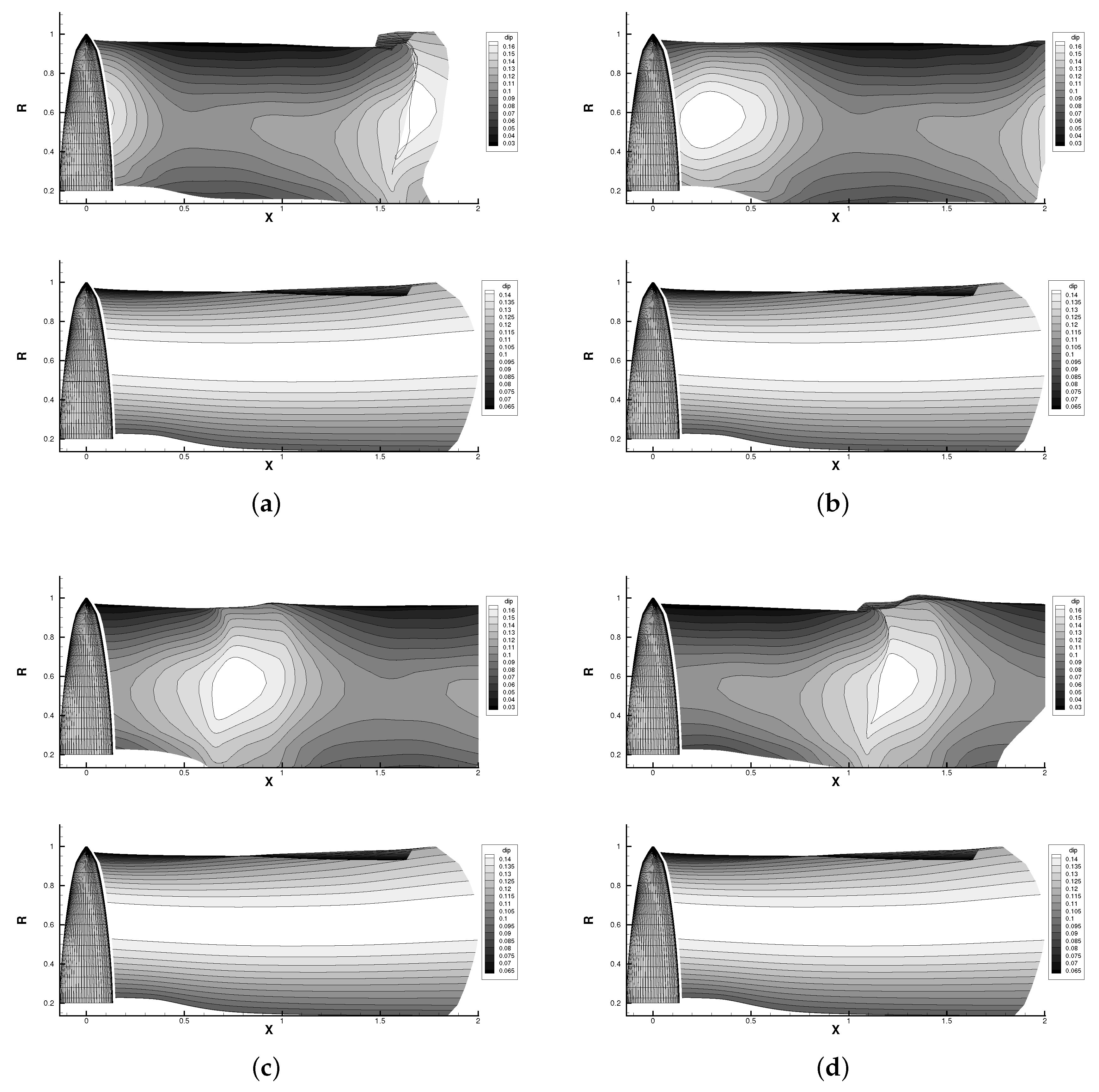
Figure 3.
Schematics showing the wake alignment process from the time step t (dashed line mesh) to (solid line mesh). Wake panels convect downstream with time.
Figure 3.
Schematics showing the wake alignment process from the time step t (dashed line mesh) to (solid line mesh). Wake panels convect downstream with time.

Figure 4.
NACA16006 hydrofoil at and (corresponding to the correct length ). (a) The resulting behavior of vs. l; (b) The predicted cavity shapes in ratio of blade radius (y-axis) for different guesses of l, obtained from Figure 4 of [22], with permission from the prime author, Spyros A. Kinnas in 2019.

Figure 5.
Schematics of tip vortex paneling at each section of the wake tip. Panel nodes are placed clockwise direction when viewed from downstream.
Figure 5.
Schematics of tip vortex paneling at each section of the wake tip. Panel nodes are placed clockwise direction when viewed from downstream.

Figure 6.
Schematics showing directions of the local velocities in s, v, and n directions on the curvilinear coordinate system. Integral in Equation (24) is computed along the positive v direction from the panel which is attached to wake tip.
Figure 6.
Schematics showing directions of the local velocities in s, v, and n directions on the curvilinear coordinate system. Integral in Equation (24) is computed along the positive v direction from the panel which is attached to wake tip.
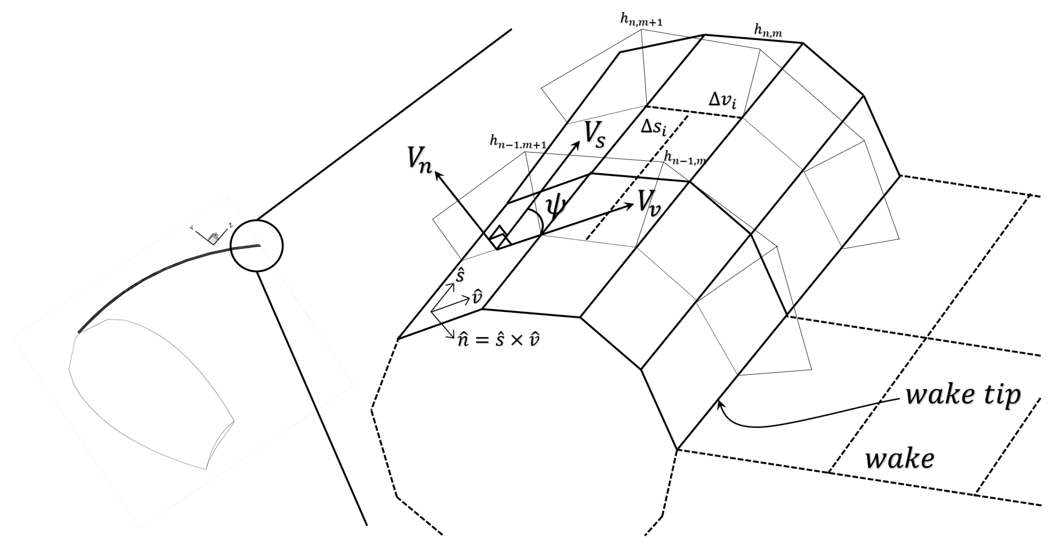
Figure 7.
Potentials around the tip vortex cavitation in connection with the wake surface (left), and its cross section view with arrangement of the potentials calculated by Equation (24) along the v direction (right).
Figure 7.
Potentials around the tip vortex cavitation in connection with the wake surface (left), and its cross section view with arrangement of the potentials calculated by Equation (24) along the v direction (right).
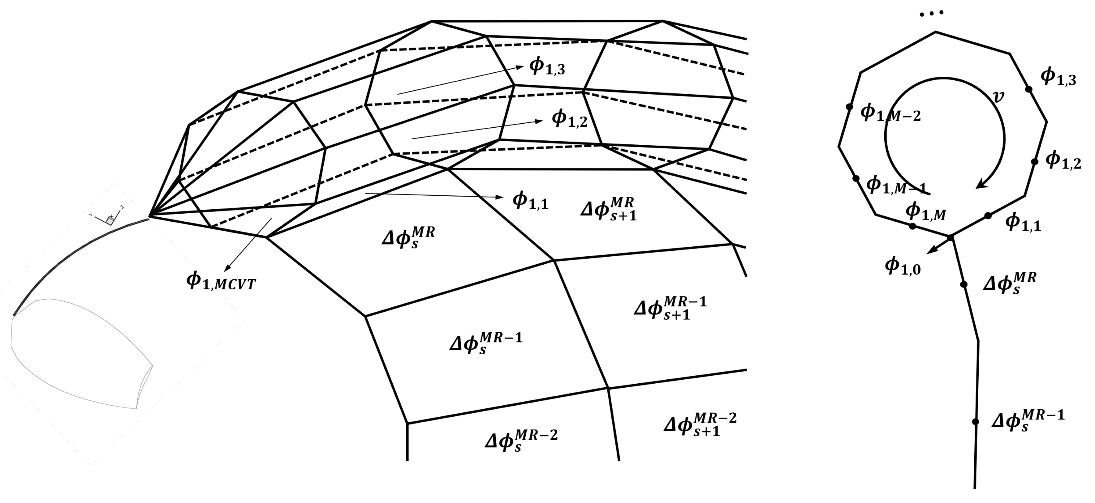
Figure 8.
Adjusting tip vortex radii from the initial shape (left). Kinematic boundary condition (Equation (27)) updates the radius in radial direction (middle), and the potential jump condition expands or contracts the overall shape, depending on the sign and the magnitude of the (right).
Figure 8.
Adjusting tip vortex radii from the initial shape (left). Kinematic boundary condition (Equation (27)) updates the radius in radial direction (middle), and the potential jump condition expands or contracts the overall shape, depending on the sign and the magnitude of the (right).
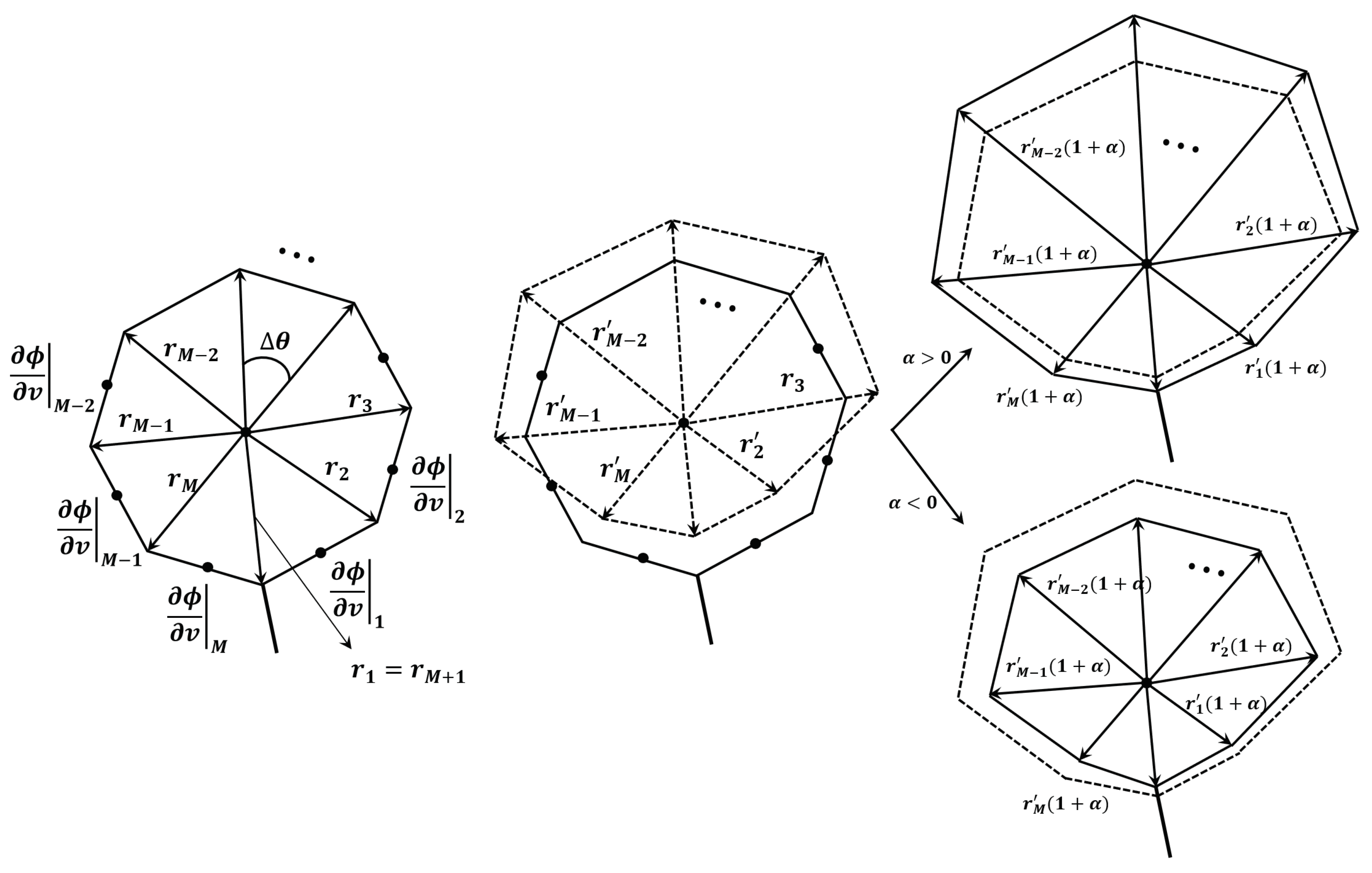
Figure 9.
Twisted tip vortex cavity sections before adjustment. The zone over which a tip vortex cavity is not considered is also shown. The criterion to determine the zone with no tip vortex cavity is .
Figure 9.
Twisted tip vortex cavity sections before adjustment. The zone over which a tip vortex cavity is not considered is also shown. The criterion to determine the zone with no tip vortex cavity is .
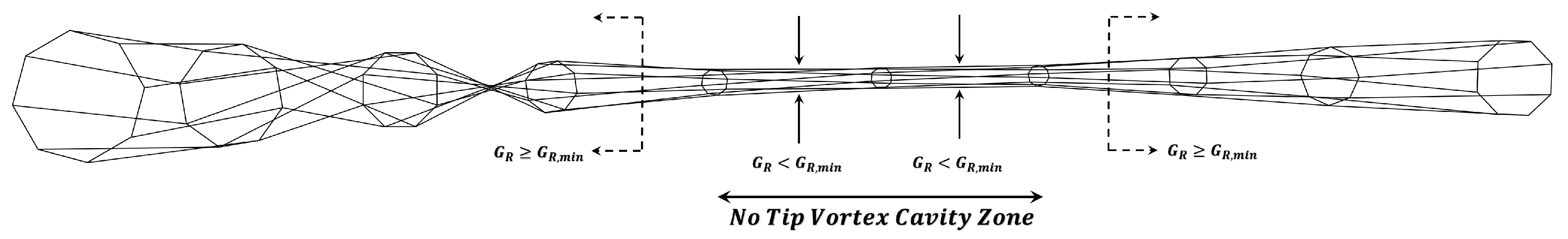
Figure 10.
Initial guess of tip vortex cavity with and the local coordinate axes along the streamline in the trailing wake and the cross flow direction, respectively (a); distortions. of tip vortex cavity panels due to the rollup in the wake (b); a non-zero dihedral angle between the two adjacent planes and (c); adjusted panel perimeters (d) and updated cavity panels (e).

Figure 11.
Projected view of the fully aligned wake (up) and its initial geometry (down), plotted on the plane at the blade angle of (a) , (b) 72°, (c) 144°, and (d) 216°.
Figure 11.
Projected view of the fully aligned wake (up) and its initial geometry (down), plotted on the plane at the blade angle of (a) , (b) 72°, (c) 144°, and (d) 216°.

Figure 12.
Projected view of the fully aligned wake of DTMB4661 propeller with hub, which has elliptical shape at both ends. Geometry of the 5-bladed propeller is shown in a separate frame.
Figure 12.
Projected view of the fully aligned wake of DTMB4661 propeller with hub, which has elliptical shape at both ends. Geometry of the 5-bladed propeller is shown in a separate frame.

Figure 13.
Predicted DTMB 4661 propeller forces by BEM using the unsteady wake alignment scheme, in comparisons with RANS results in 10° inclined shaft flow at the advance ratio of 0.8, 1.0, 1.2, and 1.4 from top to bottom lines for every pair of and .
Figure 13.
Predicted DTMB 4661 propeller forces by BEM using the unsteady wake alignment scheme, in comparisons with RANS results in 10° inclined shaft flow at the advance ratio of 0.8, 1.0, 1.2, and 1.4 from top to bottom lines for every pair of and .
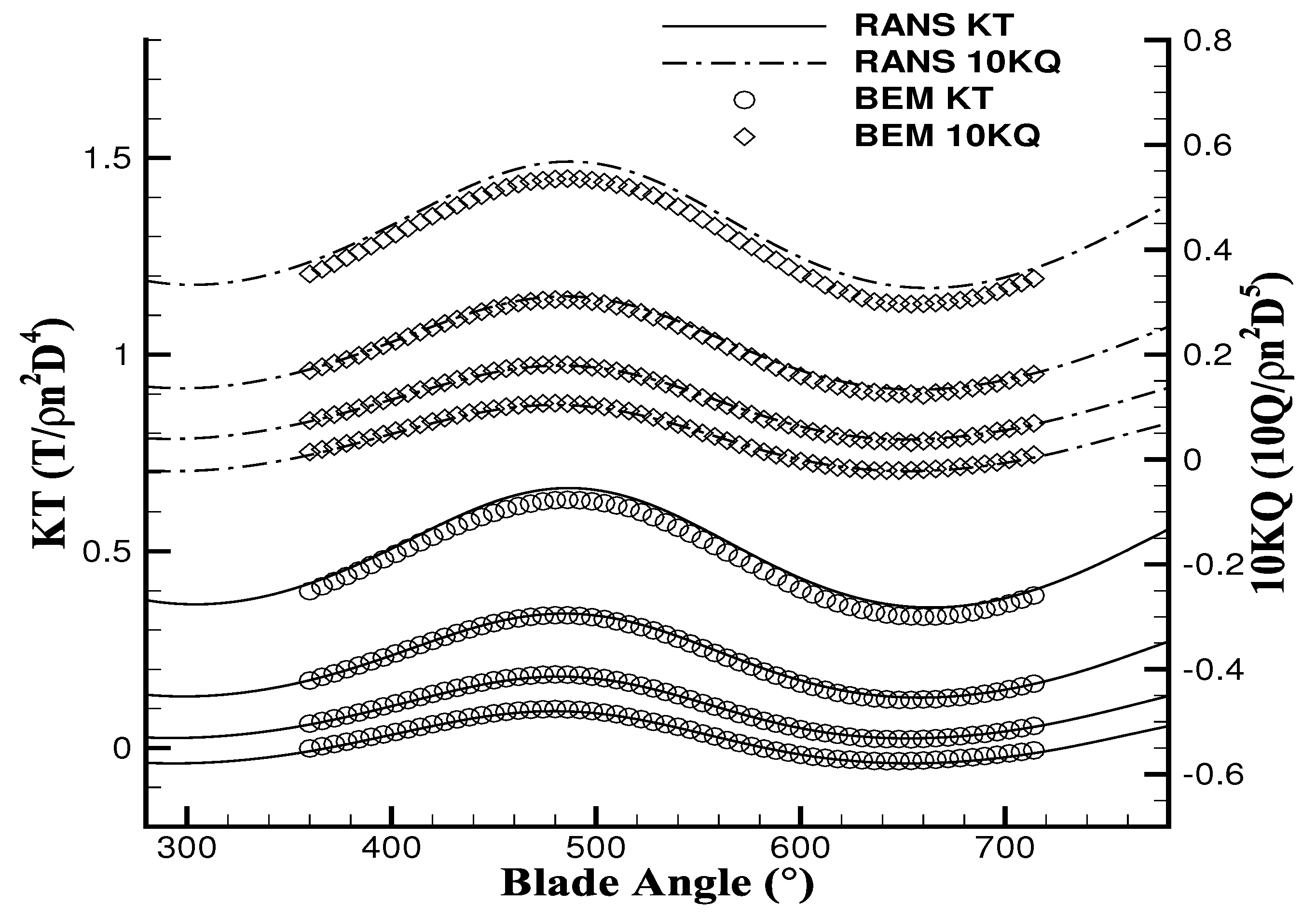
Figure 14.
Key-blade surface pressures at the four different time steps at (left) and (right). Comparisons between RANS (solid line) with BEM (symbols) in inclined shaft flow for DTMB 4661 propeller: .
Figure 14.
Key-blade surface pressures at the four different time steps at (left) and (right). Comparisons between RANS (solid line) with BEM (symbols) in inclined shaft flow for DTMB 4661 propeller: .

Figure 15.
Comparisons of the contour plots showing vorticity magnitude predicted by RANS, and the trailing wake by BEM (black solid line) for the advance ratios of (a) 0.8 and (b) 1.0. All the shown quantities and wake shapes correspond to the intersection of a vertical and a horizontal planes through the propeller axis.

Figure 16.
Geometry of DTMB N4148 propeller subject to the non-axisymmetric effective wake. Only the key wake is shown, and the wake disk is shifted upstream for clarity.
Figure 16.
Geometry of DTMB N4148 propeller subject to the non-axisymmetric effective wake. Only the key wake is shown, and the wake disk is shifted upstream for clarity.

Figure 17.
Rollup of the wake tip after the wake alignment with/without induced velocity from the tip vortex cavitation: DTMB N4148 propeller, uniform inflow. Tip cavitation geometry is not presented. The wake geometry w/o tip vortex effect is shifted by −0.5 in y direction for clarity in the lower frame.

Figure 18.
Developed tip vortex cavitation modeled by BEM during one period of propeller revolution: DTMB N4148 propeller, , . Sheet cavity on the blade is not presented.
Figure 18.
Developed tip vortex cavitation modeled by BEM during one period of propeller revolution: DTMB N4148 propeller, , . Sheet cavity on the blade is not presented.

Figure 19.
Comparisons of the blade sheet and tip vortex cavities predicted by the present method (bottom) with the measurements (top) for DTMB N4148 propeller: , , and .
Figure 19.
Comparisons of the blade sheet and tip vortex cavities predicted by the present method (bottom) with the measurements (top) for DTMB N4148 propeller: , , and .

Figure 20.
Projected view of the developed tip vortex cavitation from the BEM at blade angle on plane (up). Convergence history of the cavitation sections at the denoted downstream locations (middle). Pressure distributions on the tip cavity surface at the same locations from the initial and the converged shape (bottom).

Figure 21.
Projected view of the developed tip vortex cavitation from the BEM at blade angle on plane (up). Convergence history of the cavitation sections at the denoted downstream locations (middle). Pressure distributions on the tip cavity surface at the same locations from the initial and the converged shape (bottom).

Figure 22.
Projected view of the developed tip vortex cavitation from the BEM at blade angle on plane (up). Convergence history of the cavitation sections at the denoted downstream locations (middle). Pressure distributions on the tip cavity surface at the same locations from the initial and the converged shape (bottom).
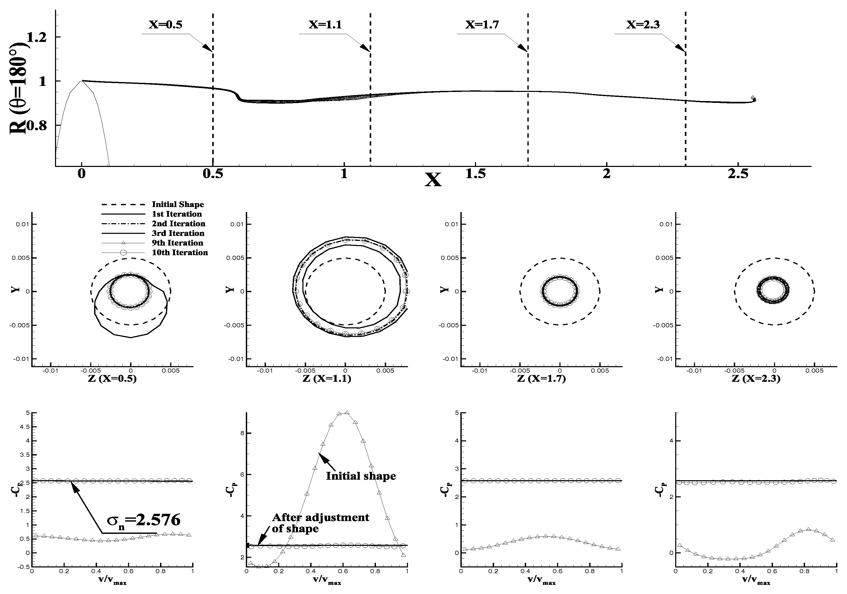
Figure 23.
Projected view of the developed tip vortex cavitation from the BEM at blade angle on plane (up). Convergence history of the cavitation sections at the denoted downstream locations (middle). Pressure distributions on the tip cavity surface at the same locations from the initial and the converged shape (bottom).

Figure 24.
SSPA P2772 propeller mounted on a model-scaled ship in the cavitation tunnel (up). Arrangement of the pressure transducers on the hull surface viewed from tunnel ceiling (down).
Figure 24.
SSPA P2772 propeller mounted on a model-scaled ship in the cavitation tunnel (up). Arrangement of the pressure transducers on the hull surface viewed from tunnel ceiling (down).
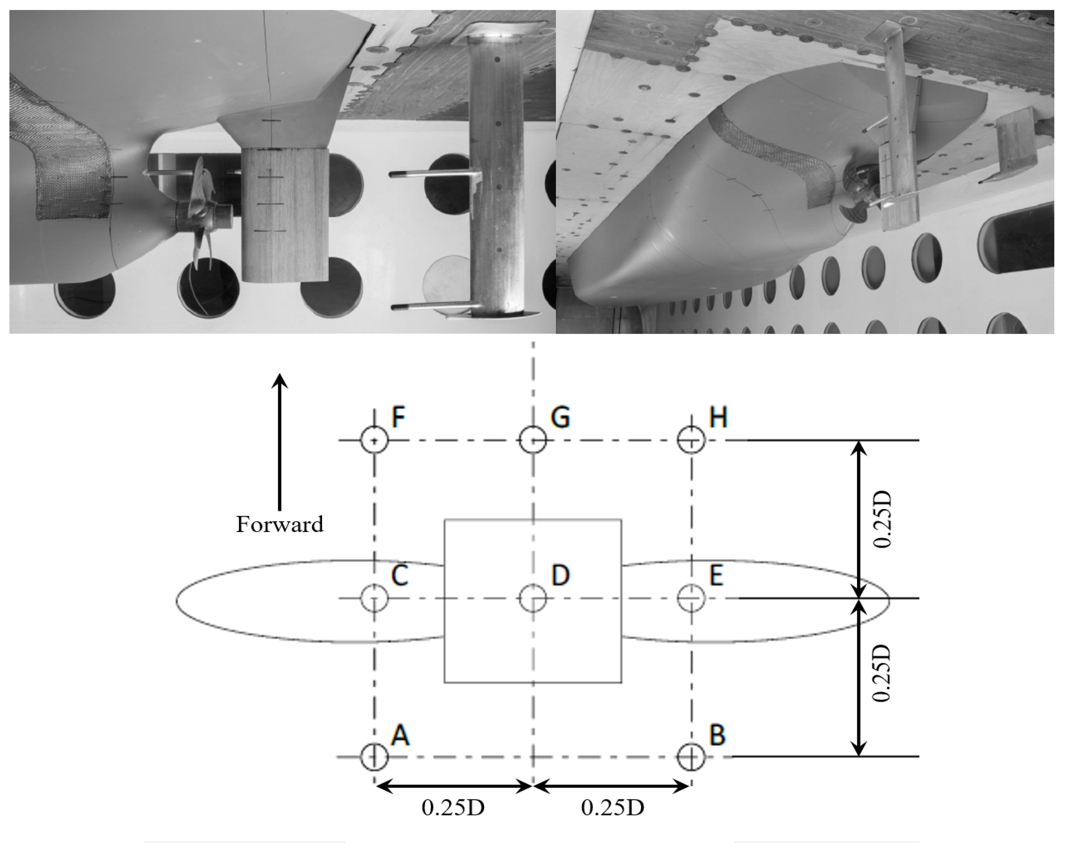
Figure 25.
Computational domain of RANS model in the BEM/RANS coupling method (left). Non-axisymmetric effective wake predicted by the same method at (right). The effective wake is evaluated on the mid-chord disk; therefore, the actual effective wake may vary in the axial direction. Axial component is represented by contour plot, and the in-plane velocities are presented by arrows.

Figure 26.
Open water characteristics of P2772 propeller predicted by BEM and the model scale experiment; ().
Figure 26.
Open water characteristics of P2772 propeller predicted by BEM and the model scale experiment; ().
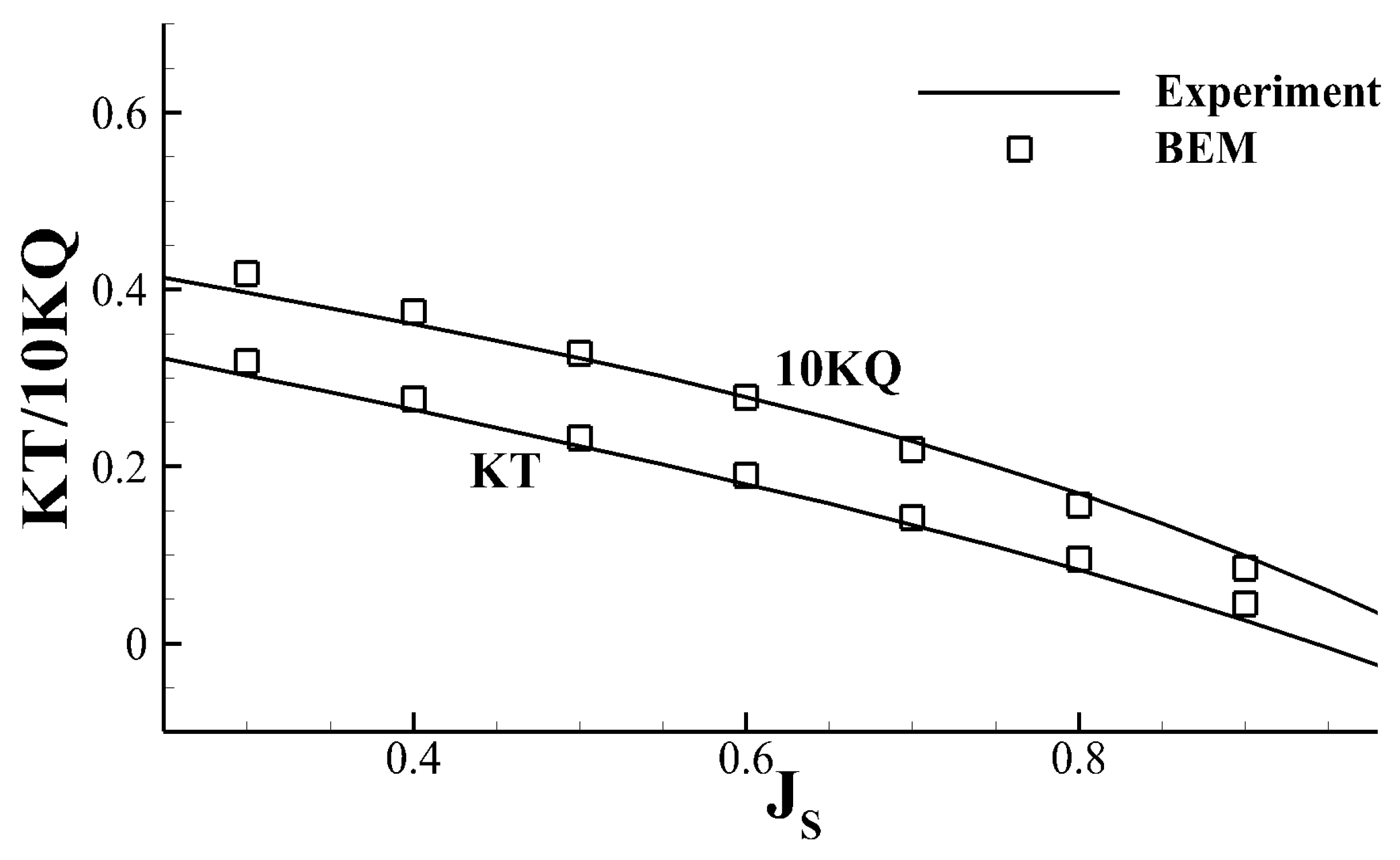
Figure 27.
Pressure-BEM model without rudder geometry. Contour plot represents the dimensionless propeller-induced hull pressures () at time step . The fore part of the hull is neglected for the sake of the efficient computation. The panels on the image model are not shown for transparency.
Figure 27.
Pressure-BEM model without rudder geometry. Contour plot represents the dimensionless propeller-induced hull pressures () at time step . The fore part of the hull is neglected for the sake of the efficient computation. The panels on the image model are not shown for transparency.

Figure 28.
Fully aligned wake of SSPA P2772 propeller with infinite hub at the blade angle (a) 0°, (b) 90°, (c) 180°, and (d) 270° positions. Only the key wake is shown.
Figure 28.
Fully aligned wake of SSPA P2772 propeller with infinite hub at the blade angle (a) 0°, (b) 90°, (c) 180°, and (d) 270° positions. Only the key wake is shown.

Figure 29.
Developed tip vortex cavitation modeled by the BEM during one propeller revolution; SSPA P2772 propeller, , .
Figure 29.
Developed tip vortex cavitation modeled by the BEM during one propeller revolution; SSPA P2772 propeller, , .
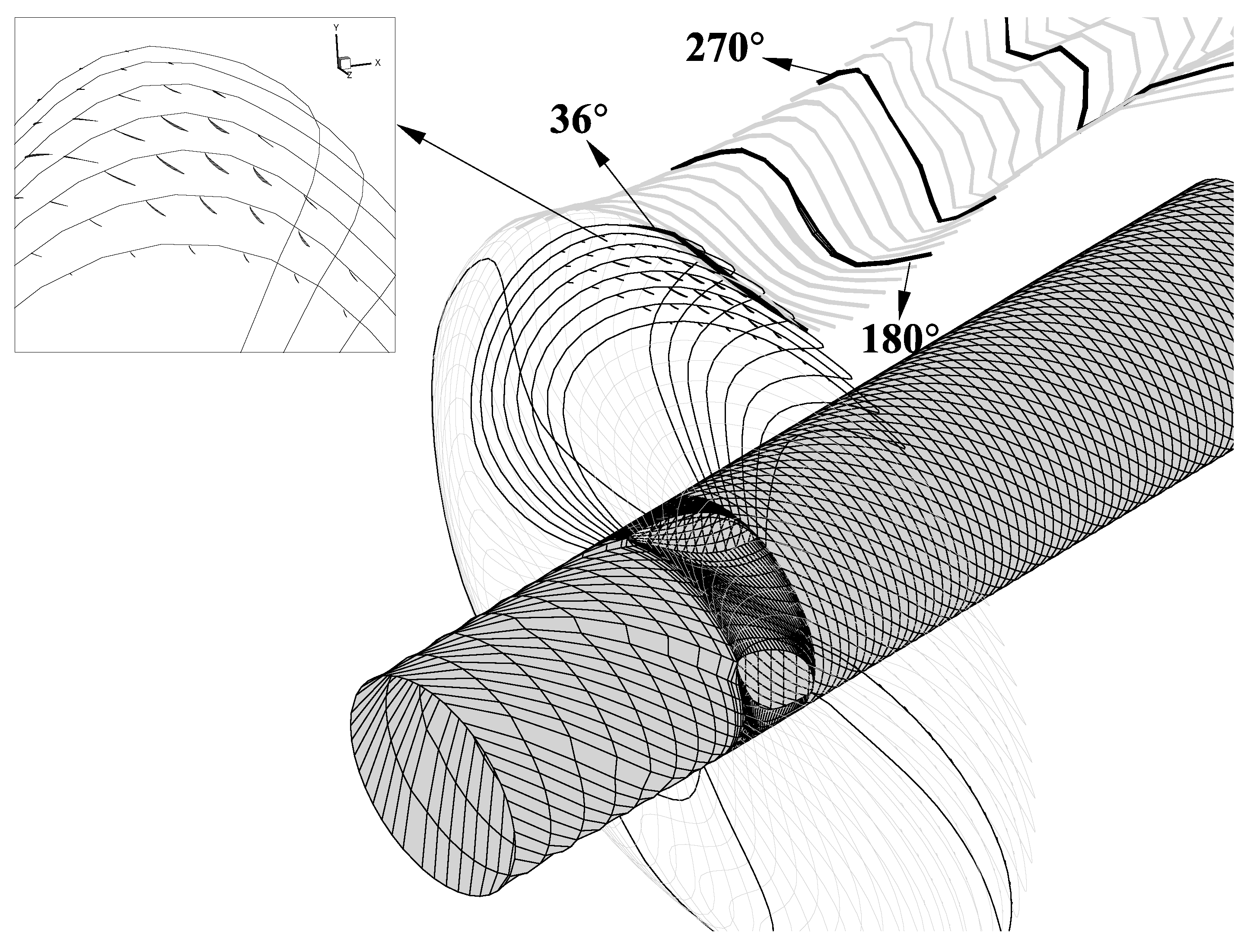
Figure 30.
Comparisons of the tip vortex caivty predicted by BEM (bottom of every pair) with the experiments for SSPA P2772 propeller; Key blade angle: (a) 340°, (b) 0°, (c) 20°, (d) 40°, (e) 60°, and (f) 80°.
Figure 30.
Comparisons of the tip vortex caivty predicted by BEM (bottom of every pair) with the experiments for SSPA P2772 propeller; Key blade angle: (a) 340°, (b) 0°, (c) 20°, (d) 40°, (e) 60°, and (f) 80°.
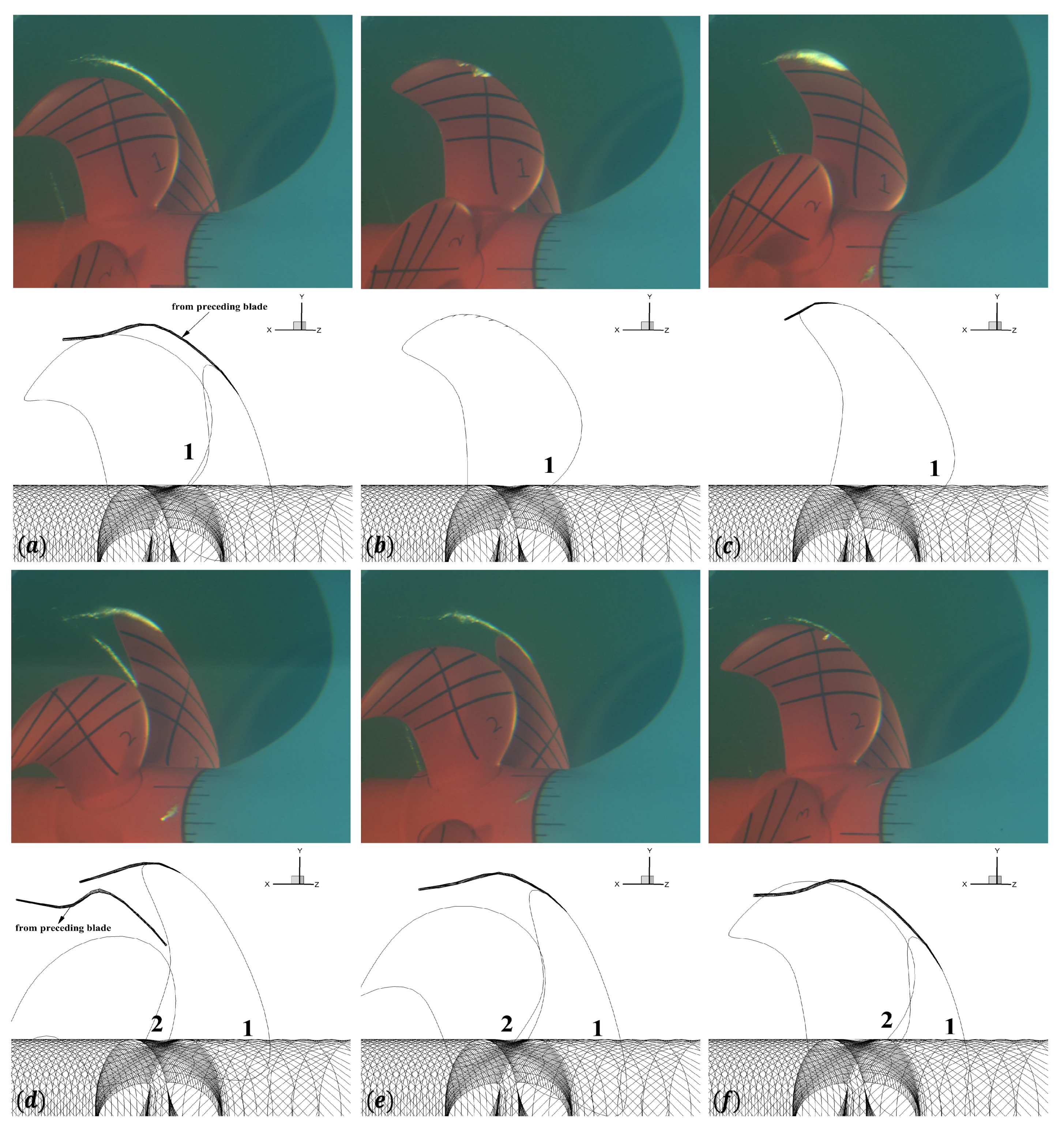
Figure 31.
Grids on the hull geometry with (left) and without (right) rudder. Transducer locations are denoted in black scatters. Propeller mesh is omitted in the figure.
Figure 31.
Grids on the hull geometry with (left) and without (right) rudder. Transducer locations are denoted in black scatters. Propeller mesh is omitted in the figure.

Figure 32.
Boundaries in the finite volume mesh used in RANS simulations for the design draft condition.
Figure 32.
Boundaries in the finite volume mesh used in RANS simulations for the design draft condition.
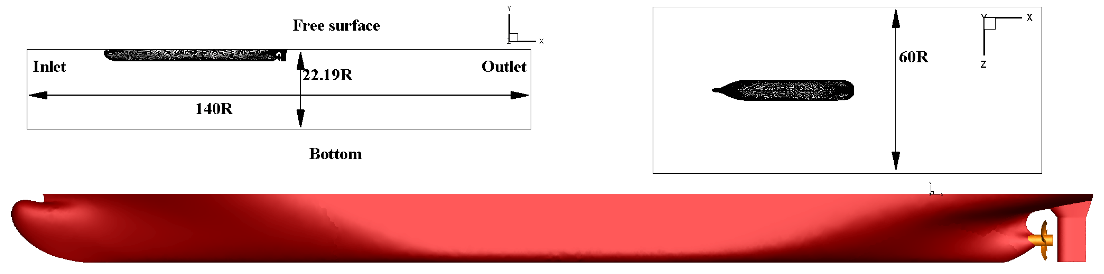
Figure 33.
Contour plots of the fluctuating hull pressures (unit: N) at the key blade angle (a) , (b) , (c) , (d) , (e) , (f) , (g) , (h) , (i) , and (j) with/without rudder. Note fluid density in RANS is to be directly compared to the BEM results. Black scatters denote the transducer locations.
Figure 33.
Contour plots of the fluctuating hull pressures (unit: N) at the key blade angle (a) , (b) , (c) , (d) , (e) , (f) , (g) , (h) , (i) , and (j) with/without rudder. Note fluid density in RANS is to be directly compared to the BEM results. Black scatters denote the transducer locations.
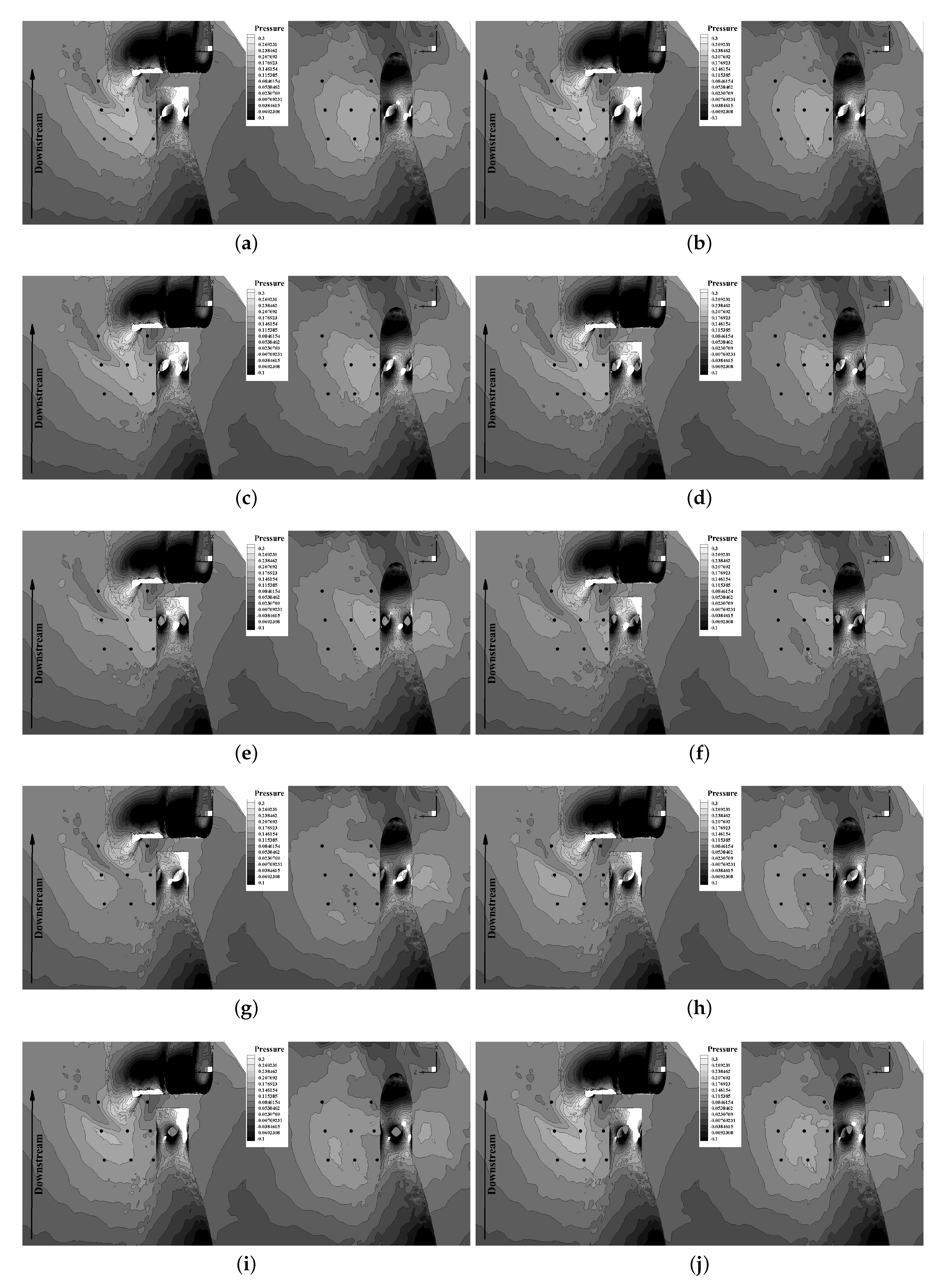
Figure 34.
Comparisons of the hull pressures (; y axis) in wetted condition between the pressure-BEM, RANS, and the experiments during the three-fourths period of propeller revolution. Results are only shown between 0° to 270° in blade angle (x axis). Locations of the transducers (A–H) are indicated in the figures.

Figure 35.
Comparisons of the hull pressures (; y axis) in cavitating conditions between the pressure-BEM and the experiments during the three-fourths period of propeller revolution. Results are only shown between 0° to 270° in blade angle (x axis). Locations of the transducers (A–H) are indicated in the figures.

Figure 36.
Comparisons of the pressure harmonics predicted by the BEM in cavitating conditions including the tip vortex cavitation model with the measurements [2].
Figure 36.
Comparisons of the pressure harmonics predicted by the BEM in cavitating conditions including the tip vortex cavitation model with the measurements [2].
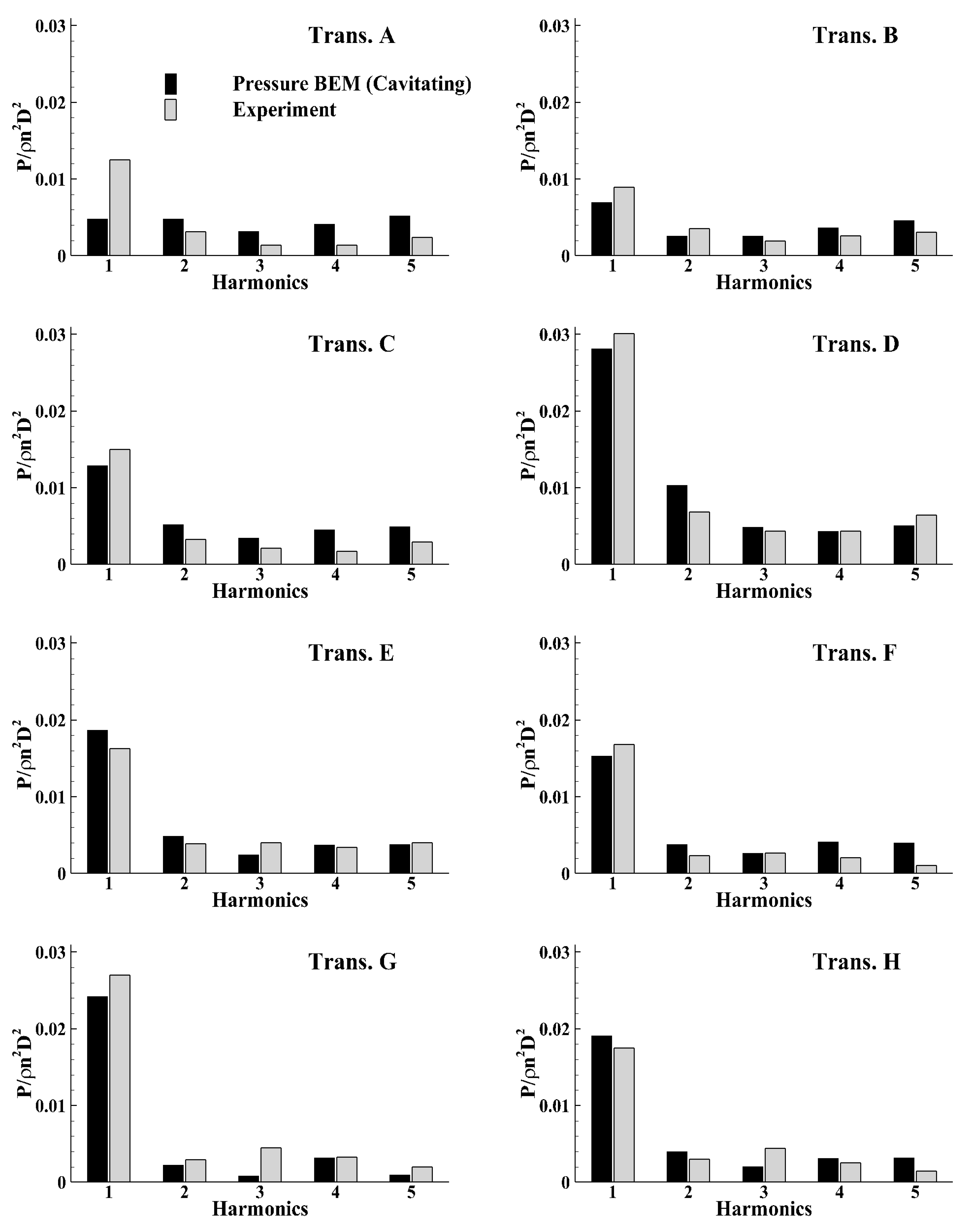
Figure 37.
Comparisons of the pressure harmonics predicted by the BEM in fully wetted condition with the measurements [2].
Figure 37.
Comparisons of the pressure harmonics predicted by the BEM in fully wetted condition with the measurements [2].


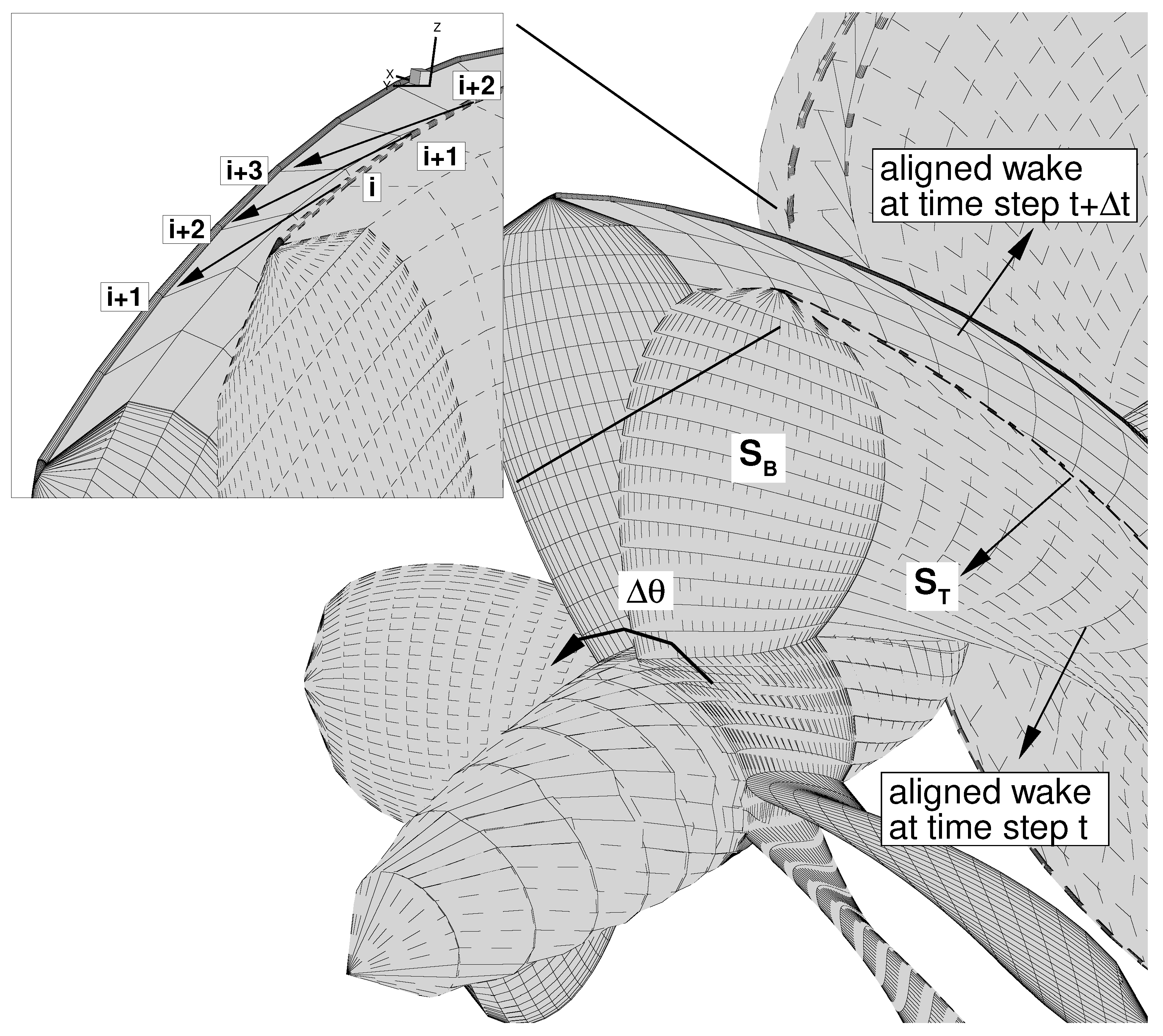
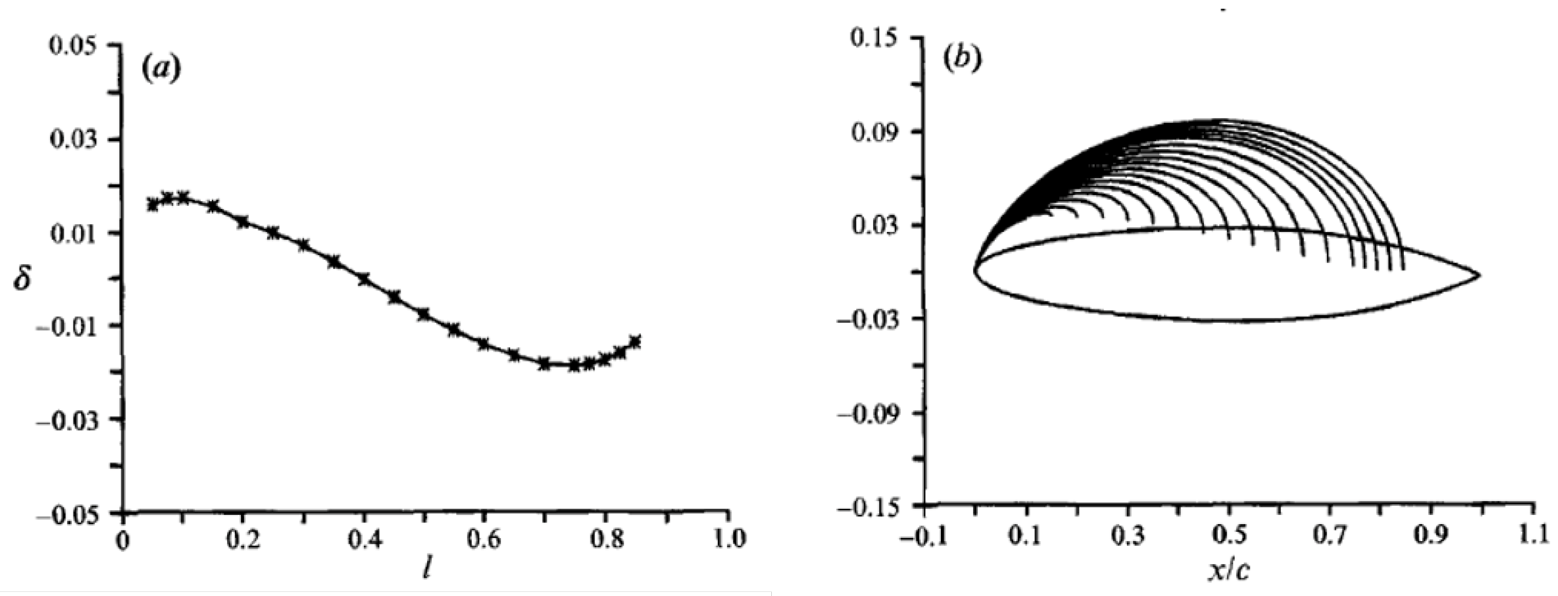
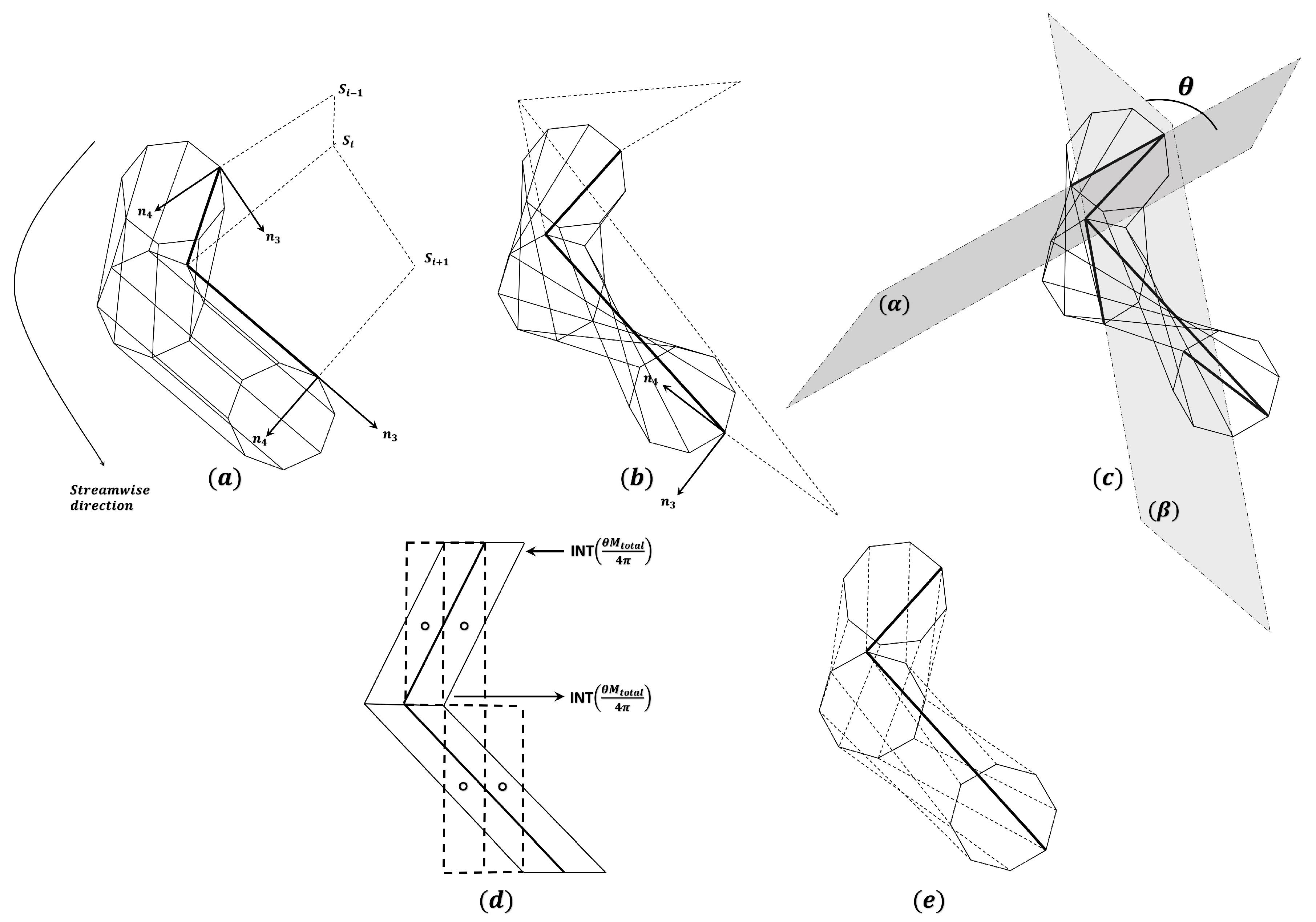
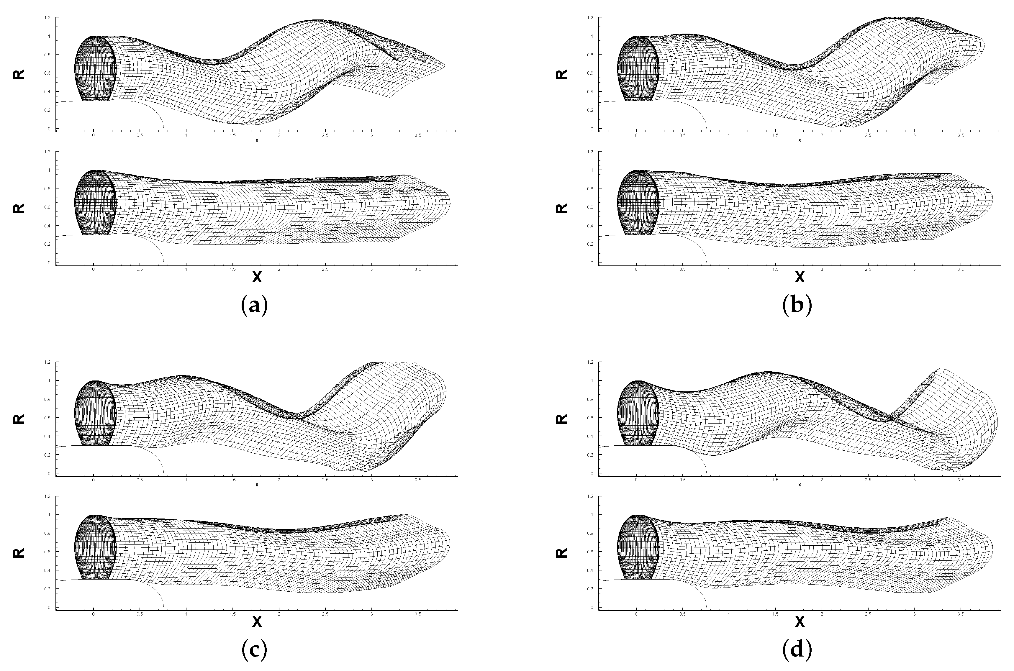
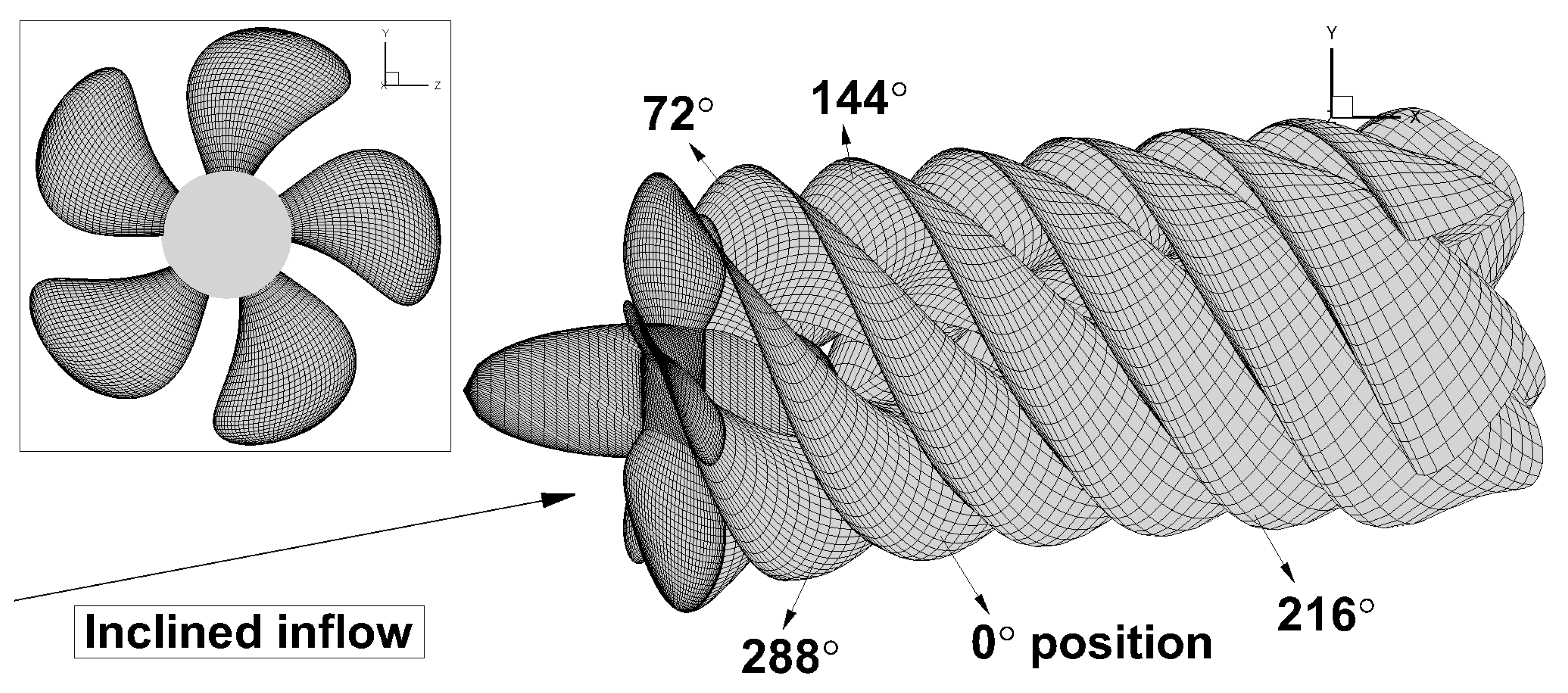
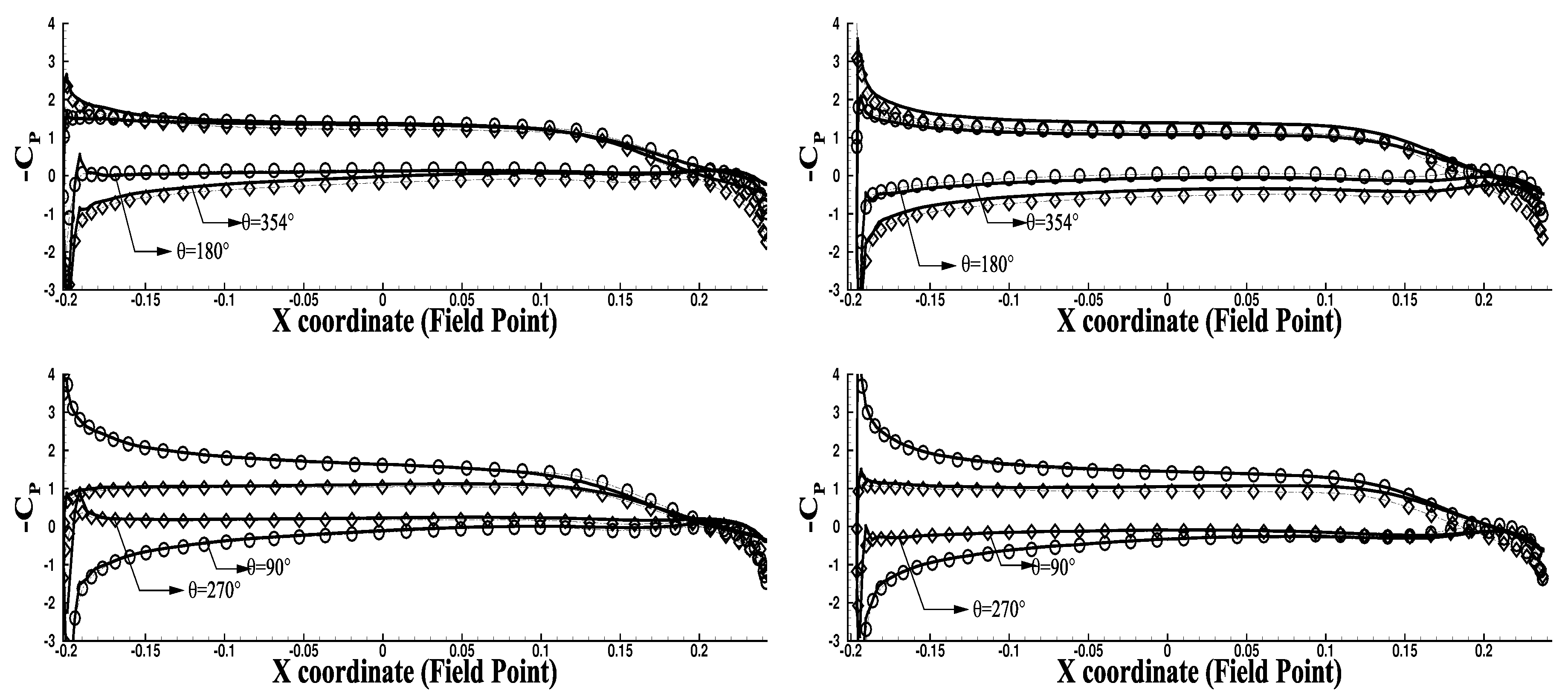
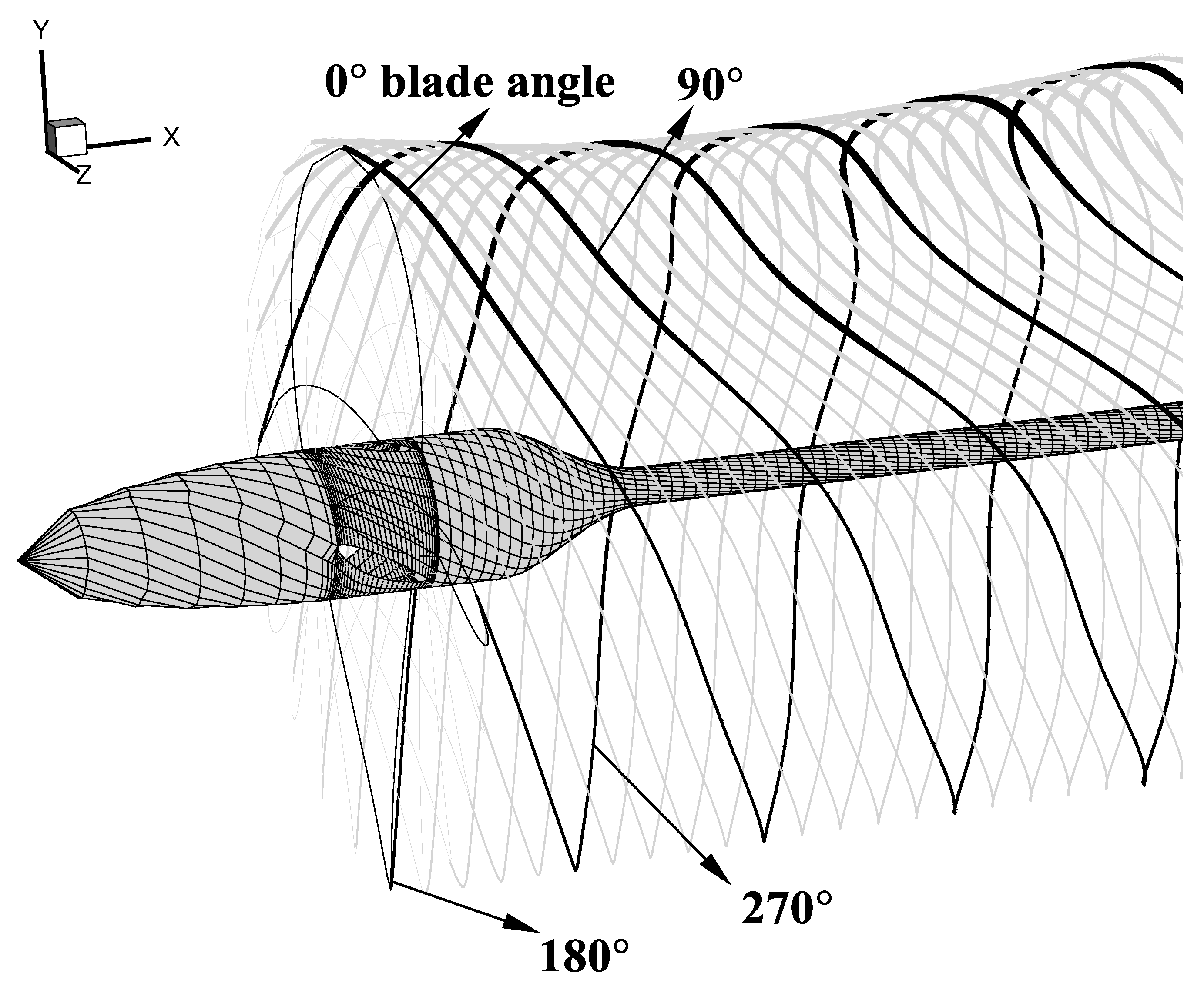
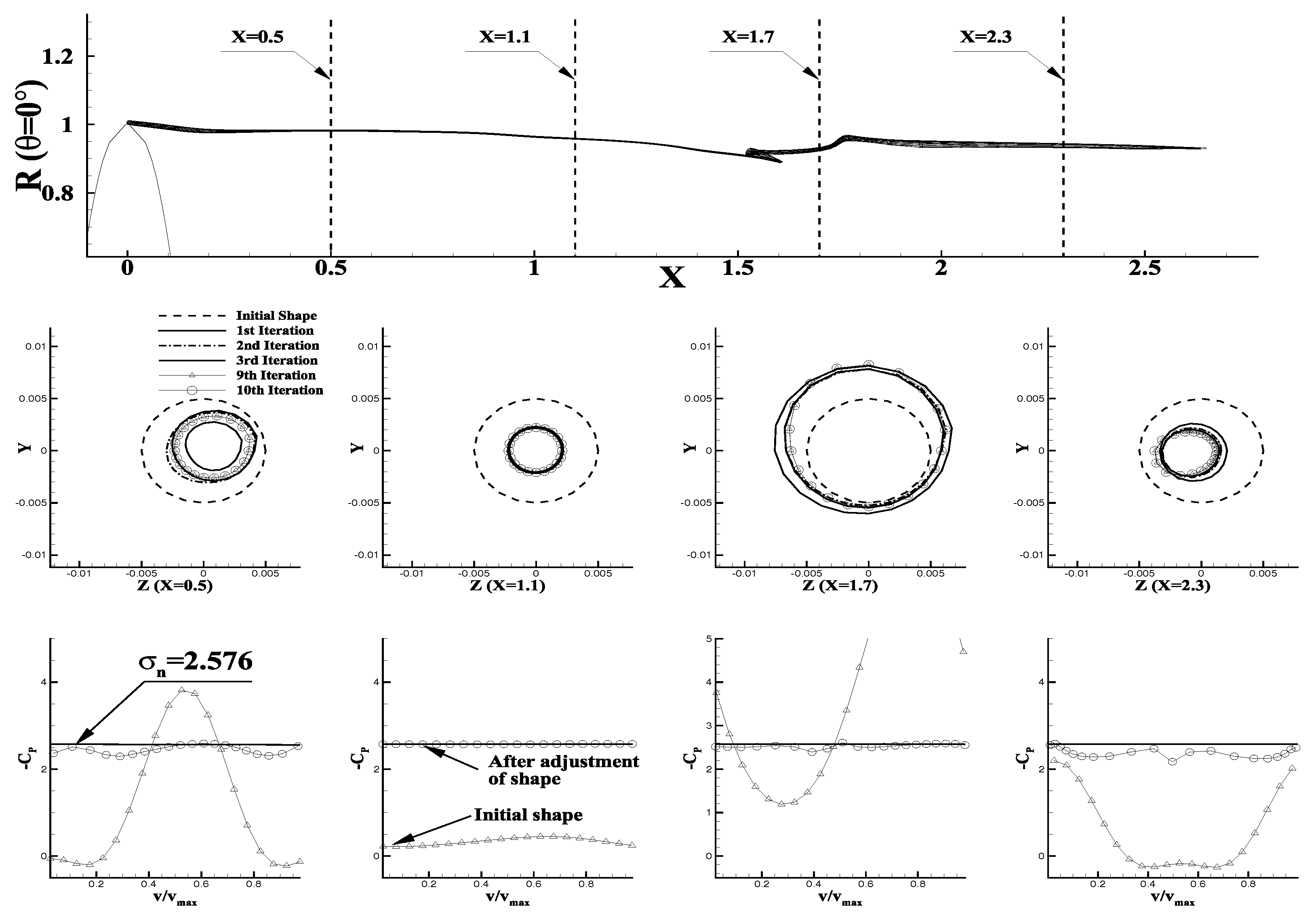
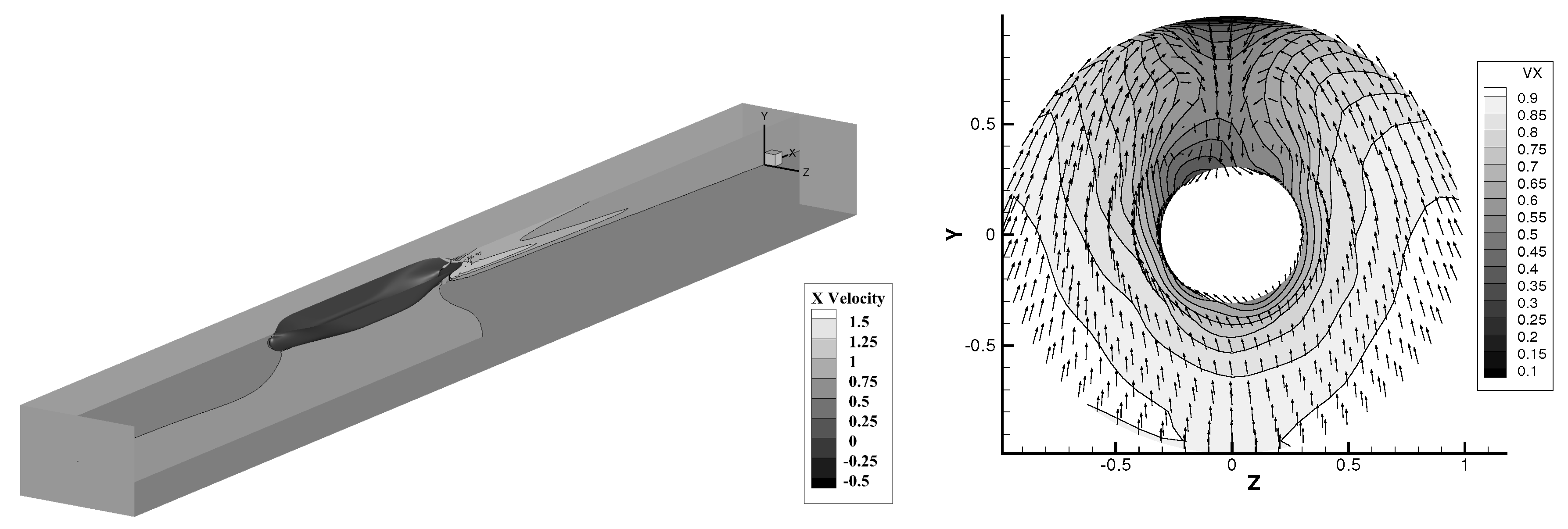
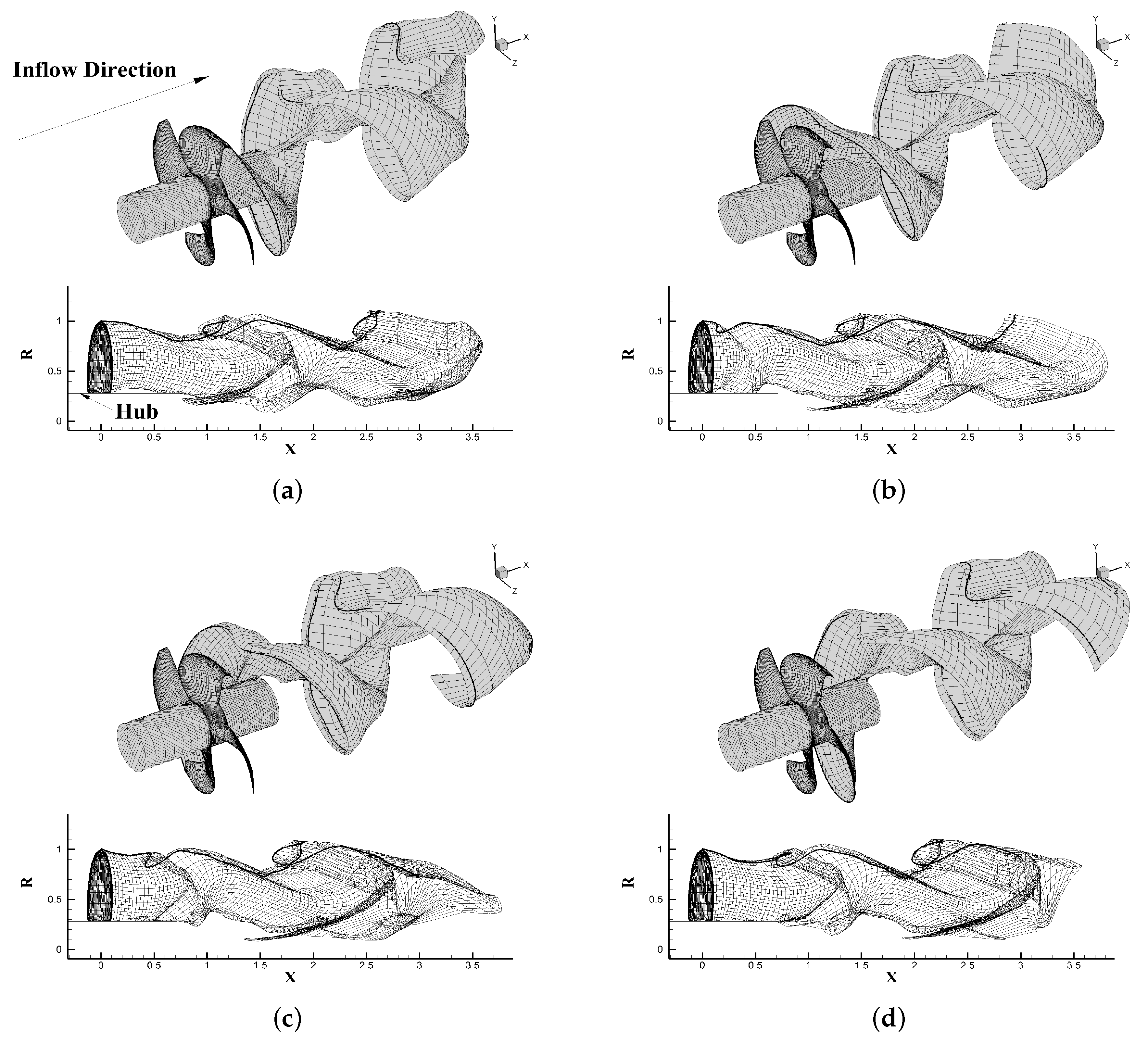
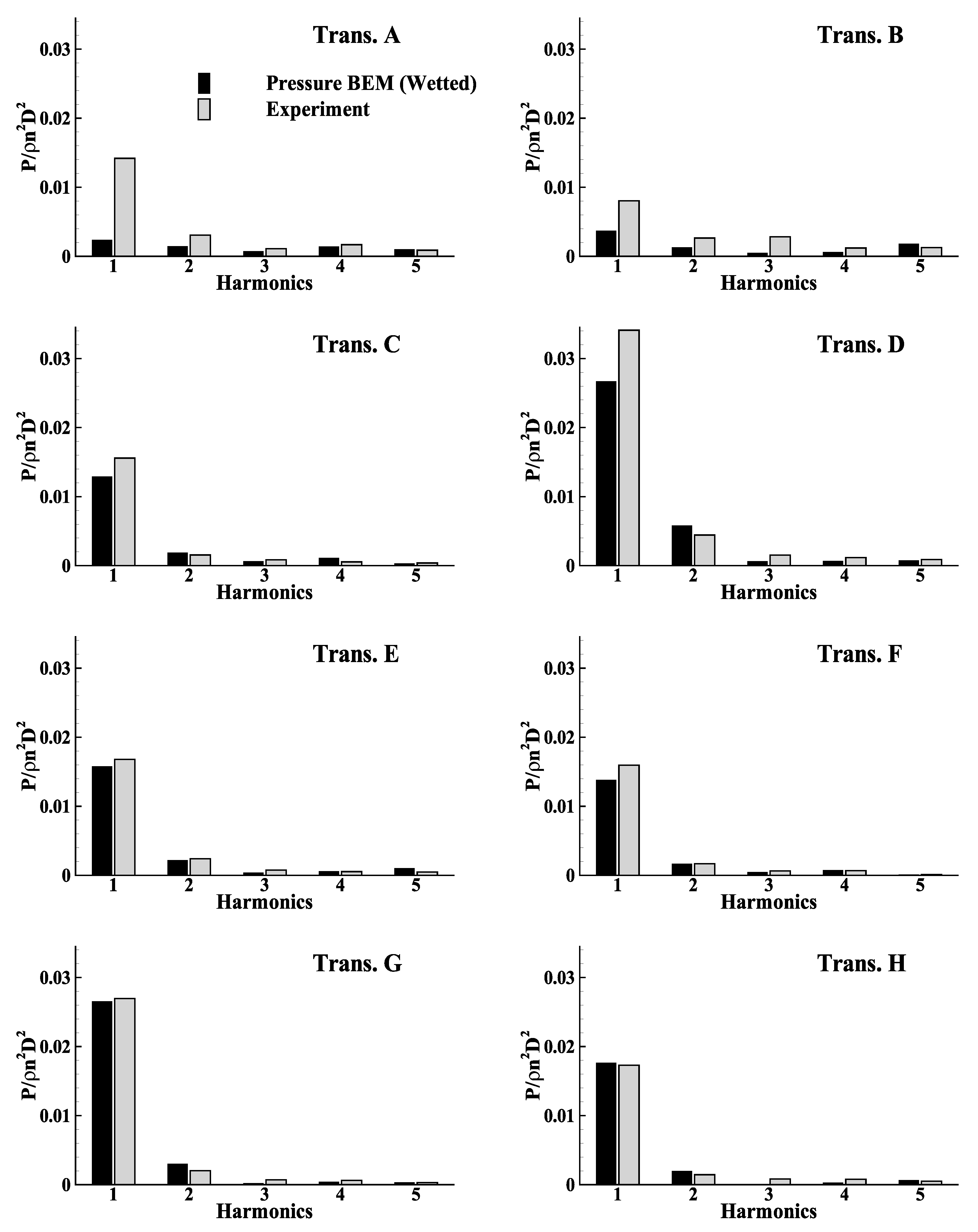
Table 1.
Applications of the numerical models in Section 3.3.
Table 1.
Applications of the numerical models in Section 3.3.
| Subsection | Propeller Geometry | Wake Field | UWA | Tip Vortex Cavitation Model | Pressure-BEM |
|---|---|---|---|---|---|
| Section 3.1 | DTMB 1 4661 | 10° inclined uniform flow | ◯ | × | × |
| Section 3.2 | DTMB N4148 | effective wake from [25] | ◯ | ◯ | × |
| Section 3.3 | SSPA P2772 [2] | effective wake from BEM/RANS coupling method | ◯ | ◯ | ◯ |
1 David Taylor Model Basin (DTMB), U.S. Navy, Maryland, U.S.
Table 2.
Loading conditions used in RANS solver.
| Advance Ratio | Propeller Diameter D | Water Density (kg/m3) | Ship Speed (m/s) |
|---|---|---|---|
| 0.7758 | 2.0 | 1.0 | 1.0 |
© 2020 by the authors. Licensee MDPI, Basel, Switzerland. This article is an open access article distributed under the terms and conditions of the Creative Commons Attribution (CC BY) license (http://creativecommons.org/licenses/by/4.0/).
Share and Cite
MDPI and ACS Style
Kim, S.; Kinnas, S.A. Prediction of Unsteady Developed Tip Vortex Cavitation and Its Effect on the Induced Hull Pressures. J. Mar. Sci. Eng. 2020, 8, 114. https://doi.org/10.3390/jmse8020114
AMA Style
Kim S, Kinnas SA. Prediction of Unsteady Developed Tip Vortex Cavitation and Its Effect on the Induced Hull Pressures. Journal of Marine Science and Engineering. 2020; 8(2):114. https://doi.org/10.3390/jmse8020114
Chicago/Turabian StyleKim, Seungnam, and Spyros A. Kinnas. 2020. "Prediction of Unsteady Developed Tip Vortex Cavitation and Its Effect on the Induced Hull Pressures" Journal of Marine Science and Engineering 8, no. 2: 114. https://doi.org/10.3390/jmse8020114
Note that from the first issue of 2016, this journal uses article numbers instead of page numbers. See further details here.