Multi-Degree of Freedom Propeller Force Models Based on a Neural Network and Regression

Abstract

Accurate and efficient prediction of the forces on a propeller is critical for analyzing a maneuvering vessel with numerical methods. CFD methods like RANS, LES, or DES can accurately predict the propeller forces, but are computationally expensive due to the need for added mesh discretization around the propeller as well as the requisite small time-step size. One way of mitigating the expense of modeling a maneuvering vessel with CFD is to apply the propeller force as a body force term in the Navier–Stokes equations and to apply the force to the equations of motion. The applied propeller force should be determined with minimal expense and good accuracy. This paper examines and compares nonlinear regression and neural network predictions of the thrust, torque, and side force of a propeller both in open water and in the behind condition. The methods are trained and tested with RANS CFD simulations. The neural network approach is shown to be more accurate and requires less training data than the regression technique.

1. Introduction

Accurately and efficiently determining the multi-degree of freedom forces on a propeller for a maneuvering vessel is challenging. Potential flow methods are inexpensive but can be less accurate than viscous methods when the propeller operates off-design. Viscous flow methods, like RANS, DES, or LES, can be more accurate than potential flow methods, but require a very small time step and require extra mesh discretization for the propeller. Common ways of modeling a discretized propeller are with the overset method or sliding mesh methods [1,2,3,4]. The cost can be prohibitive for CFD of a maneuvering vessel, especially in waves and at full scale [5]. Maintaining the accuracy of a viscous CFD method while decreasing the computational cost is desirable. One way to minimize computational cost is to determine the body force using a model. The body force can be applied to the flow and to the vessel equations of motion. This approach can be used with a constant body force [6], a database driven model [7], Boundary Element Models [8], semi-empirical methods [9,10], or by using Blade Element Momentum Theory [5,11,12,13]. Methods that ignore viscous effects may not be as accurate as modeling a fully discretized propeller with CFD in off design conditions. Despite potential loss in accuracy in off-design conditions, Boundary Element Models and Blade Element Momentum Theory are less expensive than modeling a discretized rotating propeller with CFD [8].

This paper explores the use of data-driven models that are trained with RANS CFD. The intent is for the model to be as accurate as the CFD method used to train the model. When implemented as a body force in a maneuvering analysis the model has negligible cost. There are various methods for creating data-driven models for dynamical systems ranging from regression to neural networks. Hornik et al. [14] showed that neural networks can predict any function to any requisite level of accuracy, given adequate training and inputs. Neural networks have been applied to fluid dynamics problems ranging from improved turbulence modeling [15], to determining propeller forces for different advance coefficients [16].

This paper compares the ability for regression and a neural network to predict unsteady propeller forces due to prescribed motions. The thrust T, torque Q, and side force S of a propeller with unsteady forward velocity U, side velocity V, and propeller revolution rate n are examined in this paper. Both the open water and behind condition are considered. The objective of this paper is to evaluate the capabilities of regression compared to a neural network approach for predicting the unsteady three degree of freedom body force of a propeller undergoing unsteady motions. The goal is to train a model with a small amount of training data to limit the expense. Once the model is trained, it is tested on a variety of unsteady motions to evaluate the accuracy of the model. The intent of this method is to train an algorithm with limited data and implement the algorithm to apply the body force to the flow and the forces to the equations of motion for a vessel undergoing a maneuver. This method is especially useful when it is desired to model a vessel performing different maneuvers in a variety of sea states.

The propeller examined is the National Maritime Research Institute (NMRI) scale Kriso Container Ship (KCS) propeller. Details of the CFD setup as well as the derivation for a semi-empirical propeller force method can be found in the authors’ previous work [9,17]. This paper examines both a nonlinear regression model and a neural network that are trained and tested on unsteady RANS CFD results to determine the three-degree of freedom force of the propeller in open water and the behind condition. This is an extension of the authors’ prior work in which a neural network was used to determine the three-degree of freedom force of the propeller [18].

2. Methods

Three types of analysis are used in this paper. First, the RANS CFD setup and specification of unsteady motion is discussed. Second, the neural network framework is discussed. Third, the nonlinear regression modeling is discussed.

2.1. RANS CFD Setup & Specification of Unsteady Motion

The NMRI scale KCS propeller is examined in both open water and in the behind condition. The CFD used is very similar to that used by Knight & Maki [9,17], with the only difference of using an inlet condition on the sides of the domain when there is oblique flow. The OpenFOAM solver pimpleDyMFoam is used with the sliding mesh technique used for the unsteady rotating propeller simulations. The Moving Reference Frame approach is used to calculate the steady open water propeller forces using the OpenFOAM solver simpleFoam. The $k-\omega$ SST turbulence model is used with wall functions. For the behind condition case, a symmetry plane is used at the waterline. Therefore, a double body approximation is used. The mesh used in this study correlates to the coarse grid used by Knight & Maki [9,17]. The goal is for the model to be as accurate as the method that it is trained with. Therefore, the CFD used to train and test the model is treated as the truth with regards to evaluating the accuracy of the model. In this study, RANS CFD is used to train and test the models, but other techniques, such as experimental analysis or LES, could be used instead or in conjunction.

The motions of the vessel and the propeller are prescribed using a customized OpenFOAM six degree of freedom solver. The velocity is initially accelerated from rest to the average velocity over a time $t_r$. In all cases the $t_r$ used is 0.0628 seconds. The general form of the velocity of the propeller after a time $t_r$ can be given by Equation (1). The unsteady motions are prescribed to be harmonic about the average velocity for each respective degree of freedom. Thus, the motions depend upon the average velocity ${\overline{\dot{x}}}_j$, the amplitude of motion $A_j$, the frequency of oscillation ${\omega }_{osc,j}$, and time t. The velocity amplitude ${\dot{x}}_j^{\prime }$ is the product of $A_j$ and ${\omega }_{osc,j}$. In this form, the general motions are given with subscript j. The specific degrees of motion of forward speed U, side velocity V, and revolution rate $\omega$ can be given by Equations (2)–(4), respectively. The equations are functions of the average velocities ($\overline{U}$, $\overline{V}$, and $\overline{n}$), the velocity amplitudes ($u^{\prime }$, $v^{\prime }$, and $n^{\prime }$), and time.

$${\dot{x}}_j={\overline{\dot{x}}}_j+A_j{\omega }_{osc,j}cos\left({\omega }_{osc,j}(t-t_r)\right)={\overline{\dot{x}}}_j+{\dot{x}}_j^{\prime }cos\left({\omega }_{osc,j}(t-t_r)\right)$$

(1)

$$U\left(t\right)={\dot{x}}_1=\overline{U}+u^{\prime }cos\left({\omega }_{osc,1}(t-t_r)\right)$$

(2)

$$V\left(t\right)={\dot{x}}_2=\overline{V}+v^{\prime }cos\left({\omega }_{osc,2}(t-t_r)\right)$$

(3)

$$\omega \left(t\right)=2\pi n={\dot{x}}_4=2\pi \overline{n}+2\pi n^{\prime }cos\left({\omega }_{osc,4}(t-t_r)\right)$$

(4)

2.2. Set-Up of the Neural Network for Unsteady Propeller Forces

A single hidden layer neural network is used with a sigmoid activation function. The inputs to the neural network are snapshots of the advance ratio, J, and the oblique flow angle, $\alpha$. Thus, the inputs are instantaneous feature vectors, where the feature vector includes polynomials of J and $\alpha$. The forces on the propeller depend upon the diameter of the propeller D, the density of water $\rho$, n, U, and $\alpha$. The diameter of the propeller examined is 0.105 m, and the density of the water is 997.66 kg/m${}^3$. Therefore, the output of the neural network is the instantaneous thrust coefficient, $K_T$, the instantaneous side force coefficient, $K_S$, and the instantaneous torque coefficient, $K_Q$. The equations for $K_T$, $K_S$, $K_Q$, J, and $\alpha$ are shown in Equations (5)–(9).

$$K_T=\frac{T}{\rho n^2{D}^4}$$

(5)

$$K_S=\frac{S}{\rho n^2{D}^4}$$

(6)

$$K_Q=\frac{Q}{\rho n^2{D}^5}$$

(7)

$$J=\frac{U}{nD}$$

(8)

$$\alpha ={tan}^{-1}\left(\frac{V}{U}\right)$$

(9)

The particulars of the neural network used to determine the open water propeller forces is discussed first. Second, the extension of the open water neural network to the behind condition is discussed.

2.2.1. Open Water Neural Network

A feedforward neural network with a single hidden layer is programmed in MATLAB. The input to the neural network is a feature vector, $\overrightarrow{x}$, for each snapshot in time. For each snapshot in time, the input feature vector, $\overrightarrow{x}$, is shown by Equation (10). The feature vector is comprised of permutations of the instantaneous J, up to second order, and the absolute value of $\alpha$, up to sixth order. A single hidden layer with k = 10 hidden neurons is used. The output layer has n = 3 neurons correlating to $K_T$, $K_S$, and $K_Q$, which may be scaled and shifted to improve the accuracy of the neural network.

$$\begin{array}{c}\hfill \overrightarrow{x}=[1,J,J^2{,\left|\alpha \right|,\cdots ,\left|\alpha \right|}^6{,J\left|\alpha \right|,\cdots ,J\left|\alpha \right|}^6,J^2\left|\alpha \right|,\cdots ,J^2{\left|\alpha \right|}^6{]}^T\end{array}$$

(10)

The snapshots for the training data are taken by incrementally sampling the time history of the observables of CFD simulations of an open water propeller with unsteady motions, U, V, and n. The unsteady motions are prescribed, and thus are known. Therefore, the feature vector comprised of J and $\alpha$ can be determined. The observables from the CFD simulations include the thrust, side force, and torque. These are processed to give instantaneous values of $K_T$, $K_S$, and $K_Q$. Similarly, J, $\alpha$, $K_T$, $K_S$, and $K_Q$ can all be preprocessed for the test data from CFD simulations. The force coefficients from the CFD are treated as the truth.

Based upon Equation (10), the input matrix has m = 21 rows and the number of columns equal to the number of snapshots examined. A schematic of a single hidden layer neural network is shown in Figure 1. The left hand column of neurons is the input, the middle column of neurons is the hidden layer, and the right hand column of neurons is the output layer. A sigmoid activation function is used, which is defined by Equation (11). Two weight matrices and two bias vectors are used. The first weight matrix ${\mathbf{W}}_{\mathbf{1}}$ and bias vector ${\overrightarrow{b}}_1$ are used between the input layer and the hidden layer. The second weight matrix ${\mathbf{W}}_{\mathbf{2}}$ and bias vector ${\overrightarrow{b}}_2$ are used between the hidden layer and the output layer. The values of the weight matrices and bias vectors are determined using back propagation. The accuracy for a single snapshot i can be evaluated by the loss function $L_i$ defined in Equation (12), where $\widehat{\overrightarrow{y_i}}$ is the prediction and $\overrightarrow{y_i}$ is the truth for that snapshot. $\widehat{\overrightarrow{y_i}}$ is calculated from Equation (13) which depends on the output of Equation (14).

$$\sigma \left(z\right)=\frac{1}{1+e^{-z}}$$

(11)

$$L_i=\frac{1}{2}\parallel \overrightarrow{y_i}-\widehat{\overrightarrow{y_i}}{\parallel }_2^2$$

(12)

$$\widehat{\overrightarrow{y_i}}=\sigma ({\mathbf{W}}_{\mathbf{2}}{\overrightarrow{\eta }}_i+{\overrightarrow{b}}_2)$$

(13)

$${\overrightarrow{\eta }}_i=\sigma ({\mathbf{W}}_{\mathbf{1}}{\overrightarrow{x}}_i+{\overrightarrow{b}}_1)$$

(14)

The average loss function L across all snapshots is most indicative of the error. Therefore, the loss function of each snapshot in time is calculated. The loss functions for each snapshot are summed and divided by the number of snapshots N as shown by Equation (15). The program iterates until the loss function is below a user defined tolerance. Stochastic gradient descent is used to improve the speed of convergence. The stochastic gradient descent algorithm works by randomly selecting one of the snapshots and calculating the gradients of the weight matrices based on that snapshot. Once the neural network is trained, it is tested with data from other unsteady propeller CFD simulations. The accuracy of the neural network is evaluated by how accurate it is compared to the force coefficients calculated from the CFD.

$$L=\frac{1}{N}\sum _{i=1}^N{L}_i$$

(15)

2.2.2. Extension of Neural Network to Predict Unsteady Behind Condition Propeller Forces

The neural network for the behind condition propeller forces is similar to the open water propeller neural network. For the behind condition neural network, the feature vector defined by Equation (10) is modified; the $\left|\alpha \right|$ is changed to $\alpha$. Therefore, the oblique flow angle maintains its sign. In the open water propeller case, the direction of motion did not have an effect except to determine the sign of the side force. However, in the behind condition the hull interacts with the propeller. The direction of $\alpha$ affects the propeller forces since the propeller is rotating in the wake of the hull. Equation (16) shows the feature vector used as input to the neural network for the behind condition for each snapshot in time. Note that J and $\alpha$ are calculated based upon the prescribed vessel velocities and n, just like the open water method. The high dimensionality of the feature vector allows for faster training of the model. Early stopping is used to avoid overtraining of the model. A study is performed while training the behind condition model to determine when the neural network is sufficiently trained and not overtrained.

$$\begin{array}{c}\hfill \overrightarrow{x}={[1,J,J^2,\alpha ,\cdots ,{\alpha }^6,J\alpha ,\cdots ,J{\alpha }^6,J^2\alpha ,\cdots ,J^2{\alpha }^6]}^T\end{array}$$

(16)

The second difference between the behind conditional neural network and the open water neural network is the manner in which they are trained. As aforementioned, the open water neural network uses stochastic gradient descent. The open water neural network is also trained with the results of one unsteady open water propeller CFD simulation. However, the behind condition neural network uses gradient descent instead. Therefore, the average gradient of the weights and bias vector is used to correct the current weights. The behind condition propeller neural network is trained with two different types of simulations. It uses one unsteady CFD simulation of the propeller operating in the behind condition. It also uses steady state open water propeller coefficients which are extended into the behind condition in accordance with [9,17]. Knight & Maki used the thrust identity [19] to extend steady state open water $K_T$ and $K_Q$ into $K_T$ and $K_Q$ coefficients for the propeller operating in the behind condition if the same propeller is run in the behind condition at a single U and n. The KCS propeller has been simulated using a Moving Reference Frame approach at different J values in open water and a rotating propeller simulation was performed for the propeller operating in the behind condition with constant U and n at one speed to determine the Taylor Wake fraction w using the thrust identity [19]. This parameter has been found in [9,17]. Therefore, the behind condition case is trained with the results of one unsteady behind condition propeller simulation and the open water $K_T$ and $K_Q$ values extended into the behind condition using the thrust identity.

2.3. Nonlinear Regression for Unsteady Propeller Forces

MATLAB’s non linear regression function “fitnlm” [20] is used to develop a regression model for $K_T$, $K_Q$, and $K_S$. The same training data is used for the regression model and the neural network. Thus, snapshots of a feature vector of different permutations of J and $\alpha$ are used as input. To limit the propensity for overfitting a simpler feature vector than the neural network is used. The feature vector for the regression contains terms of J and $\alpha$ up to second order, as shown in Equation (17). In the case of the open water data the absolute value of $\alpha$ is used for the same reason as for the neural network. Equation (18) shows the form of the regression model to determine the force coefficients. “fitnlm” determines the a, b, and c coefficients. In the behind condition analysis, a study is performed in which different feature vectors are used to develop the regression model.

$$\begin{array}{c}\hfill \overrightarrow{x}={[1,J,J^2,\alpha ,{\alpha }^2,J\alpha ]}^T\end{array}$$

(17)

$$\begin{array}{c}\hfill K_T=a_1+a_{2}J+a_3{J}^2+a_4\alpha +a_5{\alpha }^2+a_{6}J\alpha \\ \hfill K_S=b_1+b_{2}J+b_3{J}^2+b_4\alpha +b_5{\alpha }^2+b_{6}J\alpha \\ \hfill K_Q=c_1+c_{2}J+c_3{J}^2+c_4\alpha +c_5{\alpha }^2+c_{6}J\alpha \end{array}$$

(18)

3. Training and Testing the Neural Network and Regression Model to Predict Unsteady Open Water Propeller Forces

The models to predict unsteady open water propeller forces are trained with the results of an open water unsteady propeller CFD simulation. Discrete snapshots are examined for the training data. Before testing the neural network on a second unsteady propeller motion, a validation step is taken. The validation step examines the full time history of the unsteady propeller data that was used for training the algorithm. Once the models are trained and validated, they are tested on an unsteady propeller which undergoes a different unsteady motion.

Table 1. Open water parameters for unsteady motion.

Parameter	Train	Test
$\overline{U}$ (m/s)	1.68	1.68
$\overline{V}$ (m/s)	0.00	0.00
$\overline{n}$ (rev/s)	32.0	32.0
$u^{\prime }/\overline{U}$	0.476	0.262
$v^{\prime }/\overline{U}$	0.500	−0.476
$n^{\prime }/\overline{n}$	0.156	0.156
${\omega }_{osc,1}/\left(2\pi \overline{n}\right)$	0.020	0.020
${\omega }_{osc,2}/\left(2\pi \overline{n}\right)$	0.020	0.020
${\omega }_{osc,4}/\left(2\pi \overline{n}\right)$	0.005	0.005

shows the parameters that define the unsteady motion for each of the cases.

3.1. Training the Neural Network and Nonlinear Regression Model

Both the neural network and the nonlinear regression model are trained on a case that has unsteady velocity in all three degrees of freedom. The average forward velocity is $\overline{U}$ = 1.68 m/s, the average side velocity is $\overline{V}$ = 0 m/s, and the average propeller revolution rate is $\overline{n}$ = 32 rev/s. The amplitudes for each degree of freedom are $A_1$ = 0.2 m, $A_2$ = 0.213 m, and $A_4$ = 31.4 rad. The frequencies of oscillation are ${\omega }_{osc,1}$ = 4 rad/s, ${\omega }_{osc,2}$ = 4 rad/s, and ${\omega }_{osc,4}$ = 1 rad/s. The non-dimensionalized velocity amplitudes are $u^{\prime }/\overline{U}$ = 0.476, $v^{\prime }/\overline{U}$ = 0.500, and $n^{\prime }/\overline{n}$ = 0.156. The motion of the propeller in surge, sway, and rotational degrees of freedom is imposed in the customized OpenFOAM multi-degree of freedom solver. Similarly, since the motion is prescribed, Equations (1)–(4) can be used to extract the velocities for each degree of freedom. The first 0.1 seconds are neglected to account for the ramp time and the initial transient effects. After this time, the CFD forces are uniformly sampled to generate 70 snapshots. J and $\alpha$ for each of the snapshots are shown in Figure 2. The feature vector is generated as a function of these J and $\alpha$ values.

At each of these snapshots, the output matrix is extracted from the CFD results. As discussed earlier, each column of output from the neural network represents the predicted ${\left[K_T{K}_S{K}_Q\right]}^T$ of each snapshot. Similarly, the nonlinear regression model determines the values the values of $K_T$, $K_S$, and $K_Q$.

$K_Q$ is much smaller than $K_T$. Additionally, as $K_S$ is zero at $\alpha =0$ rad, $K_S$ can be very small. Furthermore, $K_S$ oscillates about zero depending upon the direction of the sway velocity. Therefore, for both the training and testing of the open water unsteady propeller models, scaling is applied to the $K_Q$ and $K_S$ extracted from the forces calculated by the CFD. The value of $K_S$ is also shifted to improve the scaling. $K_S$ and $K_Q$ are recast in Equations (19) and (20), where the subscript u denotes unscaled coefficients, correlating to the original $K_S$ and $K_Q$ defined in Equations (6) and (7) respectively. The absolute value of $K_{S,u}$ is used as the input matrix contains functions of the absolute value of the oblique flow angle; thus, directionality is not accounted for. It was found that the neural network was more robust when directionality was omitted in the neural network. The sign of the side force is corrected after the models calculate $K_S$. This is demonstrated when the models are tested.

$$K_S=10\left|K_{S,u}\right|+0.3$$

(19)

$$K_Q=10K_{Q,u}$$

(20)

3.1.1. Training the Neural Network for Unsteady Open Water Propeller Forces

Figure 3 shows L versus the training iteration. As stochastic gradient descent is used, the loss function may increase on some iterations, but the loss function overall tends to decrease until reaching a floor. The training loss function is reduced to 3.1 × 10${}^{-5}$. To note, the neural network was examined with the same second order feature vector used by the nonlinear regression method. Using this lower order feature vector leads to similar prediction of the forces, but requires twice as many training iterations compared to the higher order feature vector.

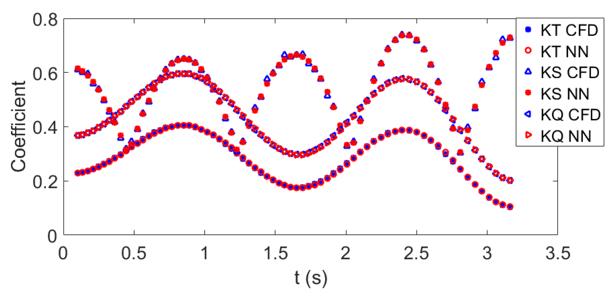
Figure 4 shows the neural network prediction for the training data. This demonstrates that the neural network is trained sufficiently, as it does a good job predicting the data that it was trained with. The neural network can further be validated by examining the neural network prediction of the coefficients versus the CFD predictions for the whole time series, instead of the 70 discrete snapshots used to train the neural network. Figure 5 shows that the neural network does a good job of predicting the force coefficients from the CFD for the whole time series. Note that the side force predicted by the CFD has a high frequency oscillation due to the side force varying as a function of the rotation angle of the propeller. However, this oscillation is not modeled by the neural network since it was not trained with the rotational position of the propeller as a feature, nor were enough snapshots used to train the neural network to discern this characteristic. This oscillation is small and since the intent of the neural network is for use in vessel maneuvering this small oscillation is not necessary to capture.

3.1.2. Training the Nonlinear Regression Model for Unsteady Open Water Propeller Forces

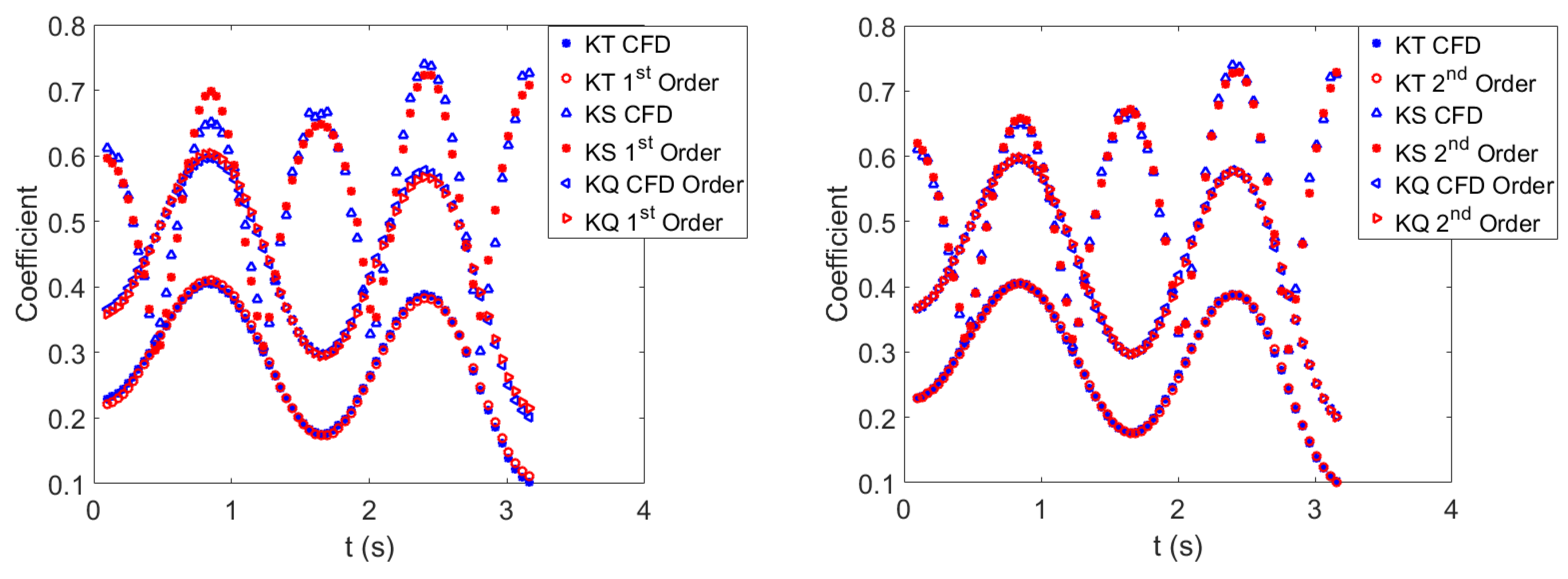
The nonlinear regression fit determined using MATLAB for the prediction of $K_T$, $K_S$, and $K_Q$ for the open water propeller is given by Equation (21). Figure 6 shows the nonlinear regression prediction for the training data. The left hand figure illustrates how well the regression model would predict the training data if only first order terms were used and the regression model was trained neglecting the $J^2$, ${\alpha }^2$, and $J\alpha$ features. The right hand image shows an improvement if the second order terms are included. This demonstrates that the nonlinear regression model is trained sufficiently when the second order features are used.

$$\begin{array}{c}\hfill K_T=0.477-0.281J-0.061J^2+0.134\left|\alpha \right|-{0.204\left|\alpha \right|}^2+0.047J\left|\alpha \right|\\ \hfill K_S=0.320-0.017J-0.126J^2+1.611\left|\alpha \right|-{0.028\left|\alpha \right|}^2+0.252J\left|\alpha \right|\\ \hfill K_Q=0.680-0.332J-0.076J^2+0.162\left|\alpha \right|-{0.291\left|\alpha \right|}^2+0.069J\left|\alpha \right|\end{array}$$

(21)

3.2. Testing the Models for Unsteady Open Water Propeller Force

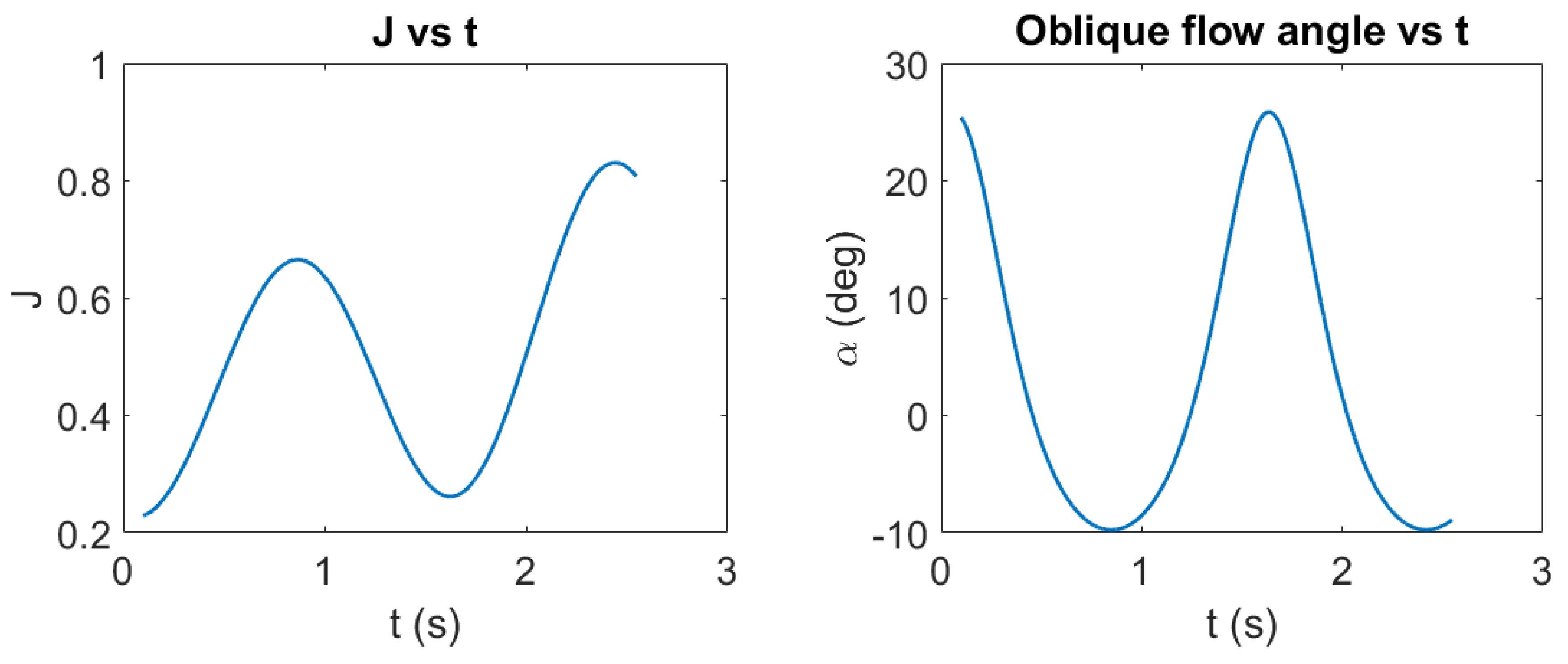
The test case has unsteady velocity in all three degrees of freedom. The average forward velocity is $\overline{U}$ = 1.68 m/s, the average side velocity is $\overline{V}$ = 0 m/s, and the average propeller revolution rate is $\overline{n}$ = 32 revolutions/s. The amplitudes for each degree of freedom are $A_1$ = 0.107 m, $A_2$ = −0.2 m, and $A_4$ = 31.4 radians. The frequencies of oscillation are ${\omega }_{osc,1}=4$ rad/s, ${\omega }_{osc,2}=4$ rad/s, and ${\omega }_{osc,1}=1$ rad/s. This results in non-dimensionalized velocity amplitudes of $u^{\prime }/\overline{U}$ = 0.262, $v^{\prime }/\overline{U}$ = −0.476, and $n^{\prime }/\overline{n}$ = 0.156. The resulting J and $\alpha$ as a function of time are shown in Figure 7.

3.2.1. Testing the Neural Network for Unsteady Open Water Propeller Force

Figure 8 shows the coefficients predicted by the neural network compared to those computed from the CFD. The average loss function is 6.56 $\times {10}^{-5}$, the average L2 norm error of the $K_T$ is 0.0035, the average L2 norm error of the $K_S$ is 0.01015, and the average L2 norm error of the $K_Q$ is 0.0040. Thus, the neural network does a good job of predicting the coefficients for the case that it was not trained with. The coefficients can be expanded back into the forces using Equations (5)–(7), (19), and (20). The sign of the side force is determined with the knowledge that the force acts in the opposite direction that the vessel sways. The side force predicted by the CFD oscillates as a function of the azimuthal position of the propeller. This high frequency oscillation is ignored by the model, as the time scale of this oscillation and the low amplitude of this oscillation will have negligible effect on the maneuvering characteristics of a vessel. The thrust, side force, and torque are plotted in Figure 9. Good agreement is seen between the forces predicted by the CFD and the neural network.

3.2.2. Testing the Nonlinear Regression for Unsteady Open Water Propeller Force

The coefficients predicted by the nonlinear regression model are quite accurate compared to those computed from the CFD. The average loss function is 5.13 $\times {10}^{-5}$, the average L2 norm error of the $K_T$ is 0.0038, the average L2 norm error of the $K_S$ is 0.00385, and the average L2 norm error of the $K_Q$ is 0.0077. Thus, the nonlinear regression also does a good job of predicting the coefficients of the test data. The average loss function and $K_S$ are predicted better using the nonlinear regression, but the $K_T$ and $K_Q$ are predicted better using the neural network. The differences in prediction between the neural network and the nonlinear regression are quite small in this case. The coefficients determined by nonlinear regression are expanded back into the forces using Equations (5)–(7), (19), and (20). The thrust, side force, and torque are plotted in Figure 10. Good agreement is seen between the forces predicted by the CFD and the nonlinear regression.

4. Training and Testing the Neural Network and Nonlinear Regression to Predict Unsteady Behind Condition Propeller Forces

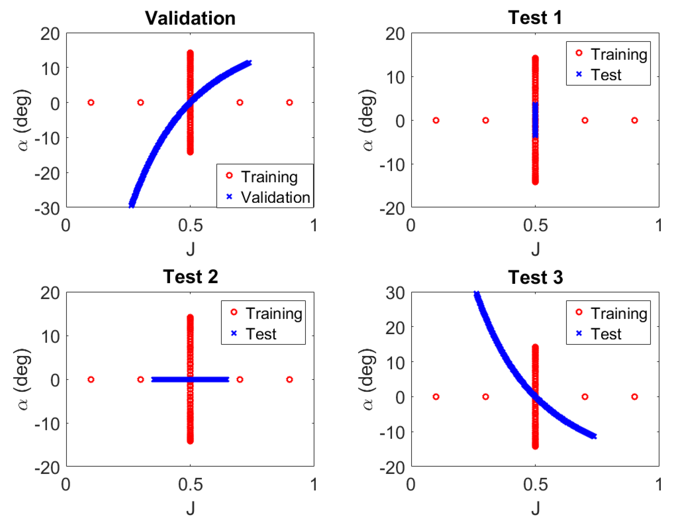
The neural network and nonlinear regression model are used to predict unsteady behind condition propeller forces. First, the models are trained with the results of a behind condition unsteady propeller CFD simulation and the steady state open water coefficients extended to the behind condition. Discrete snapshots are examined for the training data. Once the models are trained they are tested with several different unsteady behind condition propeller CFD cases that have various motions. These three different cases are denoted “Test 1”, “Test 2”, and “Test 3”.

Table 2. Behind condition parameters for unsteady motion.

Parameter	Train	Validation	Test 1	Test 2	Test 3
$\overline{U}$ (m/s)	1.68	1.68	1.68	1.10	1.68
$\overline{V}$ (m/s)	0.00	0.00	0.00	0.00	0.00
$\overline{n}$ (rev/s)	32.00	32.00	32.00	20.95	32.00
$u^{\prime }/\overline{U}$	0.00	0.48	0.00	0.31	0.48
$v^{\prime }/\overline{U}$	0.25	0.30	0.07	0.00	−0.30
$n^{\prime }/\overline{n}$	0.00	0.00	0.00	0.00	0.00
${\omega }_{osc,j}$ (rad/s)	1.00	1.00	1.00	6.72	1.00

shows the parameters that define the unsteady motion for each of the cases. Figure 11 shows $\alpha$-J space for the validation and test cases compared to the training space.

4.1. Training the Models to Predict the Unsteady Behind Condition Propeller Force

The training data is split into two parts. The first part is the unsteady behind condition propeller training case. The average forward velocity is $\overline{U}$ = 1.68 m/s, the average side velocity is $\overline{V}$ = 0 m/s, and the average propeller revolution rate is $\overline{n}$ = 32 rev/s or ${\dot{x}}_{4,avg}$ = 201.06 rad/s. The amplitudes for each degree of freedom are $A_1$ = 0 m, $A_2$ = 0.4265 m, and $A_4$ = 0 rad. The amplitude of sway is equal to the maximum waterline beam (BWL). Therefore, only the sway degree of freedom is unsteady. The resulting velocity amplitudes are $u^{\prime }$ = 0 m/s, $v^{\prime }$ = 0.42 m/s, and $n^{\prime }$ = 0 rev/s. The frequency of oscillation is ${\omega }_{osc,2}$ = 1 rad/s. The second half of the training data is the steady state open water propeller coefficients which are converted to the behind condition coefficients using the thrust identity. Therefore, the $K_T$ and $K_Q$ for steady-state open water J values of [0.1, 0.3, 0.5, 0.7 and 0.9] are expanded to the behind condition if the vessel has the same U and n used for those open water coefficients. The $K_S$ is assumed to be zero, as without drift the side force is small and this eliminates the need to perform additional behind condition simulations. This series is repeated twenty times so that the unsteady data and the steady data have similar data sizes for the determination of the training of the models.

The behind condition coefficients are scaled differently than for the open water case. $K_T$ is shifted up by 0.2 as shown by Equation (22). $K_S$ is multiplied by five and is shifted up 0.5 as shown by Equation (23). $K_Q$ follows the same scaling as in the open water modeling, shown by Equation (20).

$$K_T=K_{T,u}+0.2$$

(22)

$$K_S=5\left|K_{S,u}\right|+0.5$$

(23)

4.1.1. Training the Neural Network for the Unsteady Behind Condition Propeller Force

As noted in the open water discussion, the feature vector defined by Equation (10) trains the neural network faster than a lower order feature vector. To avoid over training the neural network, different tolerances of L are examined and are evaluated by a single test case used to validate the model. As the tolerance of L decreases, it is expected that the accuracy of the model improves until it reaches a point where the neural network may become overtrained.

The “Validation” data set is used to validate the behind condition neural network to evaluate whether or not the model is overtrained. The average forward velocity is $\overline{U}$ = 1.68 m/s, the average side velocity is $\overline{V}$ = 0 m/s, and the average propeller revolution rate is $\overline{n}$ = 32 rev/s. The resulting velocity amplitudes are $u^{\prime }$ = 0.81 m/s, $v^{\prime }$ = 0.50 m/s, and $n^{\prime }$ = 0 rev/s. The frequency of oscillation is ${\omega }_{osc,1}$ = ${\omega }_{osc,2}$ = 1 rad/s. This data set is used to validate the model since it incorporates both unsteady J and unsteady $\alpha$. The validation results for five different tolerances of L are presented: 1 $\times {10}^{-3}$, 5 $\times {10}^{-4}$, 1 $\times {10}^{-4}$, 8.3 $\times {10}^{-5}$, and 7.7 $\times {10}^{-5}$. The L as well as the L2 norm error of $K_T$, $K_S$, and $K_Q$ are shown in

Table 3. L2 norm error for different tolerances of L for validation of neural network for behind condition forces.

Train L	L2 Error ${\mathit{K}}_{\mathit{T}}$	L2 Error ${\mathit{K}}_{\mathit{S}}$	L2 Error ${\mathit{K}}_{\mathit{Q}}$	Validation L
1.0 $\times {10}^{-3}$	2.8 $\times {10}^{-2}$	5.3 $\times {10}^{-2}$	1.0 $\times {10}^{-1}$	1.0 $\times {10}^{-2}$
5.0 $\times {10}^{-4}$	1.2 $\times {10}^{-2}$	4.7 $\times {10}^{-2}$	2.4 $\times {10}^{-2}$	1.5 $\times {10}^{-3}$
1.0 $\times {10}^{-4}$	2.4 $\times {10}^{-2}$	2.6 $\times {10}^{-2}$	3.4 $\times {10}^{-2}$	1.1 $\times {10}^{-3}$
8.3 $\times {10}^{-5}$	9.6 $\times {10}^{-3}$	1.9 $\times {10}^{-2}$	8.8 $\times {10}^{-3}$	2.58 $\times {10}^{-4}$
7.7 $\times {10}^{-5}$	8.3 $\times {10}^{-3}$	1.6 $\times {10}^{-2}$	1.7 $\times {10}^{-2}$	3.0 $\times {10}^{-4}$

. The validation L is used to determine whether the neural network is appropriately trained. For these five different levels of tolerance for the training L, the optimal corresponds to a training L of 8.3 $\times {10}^{-5}$. As L is a function of all three force coefficients, it can be seen that actually the $K_T$ and $K_S$ are better predicted if a lower L tolerance is used, but the $K_Q$ gets worse. Figure 12 shows the validation force coefficients, the thrust, side force, and torque as a function of time. Each row correlates to a different training L, with L = 0.001 in the top row, and the smallest L in the bottom row. This figure illustrates how the prediction of validation forces vary as a function of the tolerance on the L used for training. A better correlation between the neural network forces and the CFD forces can be seen as the training tolerance is reduced. However, both Table 3 and Figure 12 show that as the tolerance of the training L is reduced, some forces may be better predicted in the validation set at different levels of tolerance. One way to mitigate this would be to develop a neural network specifically to determine each force. However, for the purposes of implementation as a body force in a CFD simulation, this would be less desirable due to the increased training cost.

As noted, the best tolerance found from this validation study is for L = 8.3 $\times {10}^{-5}$. Figure 13 shows the coefficients predicted by the neural network compared to those extracted from the CFD for the behind condition training case. The plot on the left shows the neural network prediction of the unsteady training data. The plot on the right shows the neural network prediction of the steady training data. Thus, this setting of L = 8.3 $\times {10}^{-5}$ leads to good results for both the training data as well as the validation test case and will be used to further test this neural network.

4.1.2. Training the Nonlinear Regression Model for the Unsteady Behind Condition Propeller Force

A study of how many features to incorporate into the regression model is performed. The validation case is used to verify the model is accurate and is used to select the number of features used to analyze the test cases. Four different forms of the regression are examined. The features examined in each of these include a second-order model, a third-order model, a fourth-order model, and a model using the neural network features. The feature vector for each of these is shown in Equation (24).

Table 4. L2 norm error for different tolerances of L for validation of neural network for behind condition forces.

Regression Model	Train L	L2 Error ${\mathit{K}}_{\mathit{T}}$	L2 Error ${\mathit{K}}_{\mathit{S}}$	L2 Error ${\mathit{K}}_{\mathit{Q}}$	Validation L
Second Order	9.3 $\times {10}^{-5}$	5.0 $\times {10}^{-2}$	1.8 $\times {10}^{-2}$	5.1 $\times {10}^{-2}$	2.7 $\times {10}^{-3}$
Third Order	7.3 $\times {10}^{-5}$	2.7 $\times {10}^{-2}$	1.4 $\times {10}^{-1}$	3.9 $\times {10}^{-2}$	1.1 $\times {10}^{-2}$
Fourth Order	7.0 $\times {10}^{-5}$	9.9 $\times {10}^{-2}$	1.4 $\times {10}^{-1}$	6.4 $\times {10}^{-2}$	1.6 $\times {10}^{-2}$
Neural Network Features	6.9 $\times {10}^{-5}$	2.0 $\times {10}^{-1}$	7.3 $\times {10}^{-1}$	5.9 $\times {10}^{-1}$	4.6 $\times {10}^{-1}$

and Figure 14 are used to evaluate the different feature vectors for the regression. Table 4 shows the training L compared to the L2 error norms of the force coefficients and the L for the validation case. This table illustrates that even though the training loss function decreases as higher features are added, the model becomes overtrained and the accuracy of the regression model on the validation test case becomes worse. This phenomenon is shown graphically in Figure 14. The top row shows the force coefficients and the forces predicted by the second order regression, the second row shows the results for the third order regression, the third row shows the results for the fourth order regression, and the last row shows the results if the feature vector used by the neural network is used. As additional terms are added to the feature vector, the prediction of the validation test case become worse. Therefore, the second-order model is used to analyze the test cases. Note that Figure 14 also shows that even the second-order model does a poor job of predicting the thrust and torque for this validation case. More training data could be used to improve the model, but that would also increase the cost of implementing the model. Therefore, it can be seen that for this set of training data, the neural network is able to do a better job of predicting the validation test case than the regression approach.

$$\begin{array}{c}\hfill \begin{array}{c}SecondOrder:\overrightarrow{x}={[1,J,J^2,\alpha ,{\alpha }^2,J\alpha ]}^T\hfill \\ ThirdOrder:\overrightarrow{x}={[1,J,J^2,J^3,\alpha ,{\alpha }^2,{\alpha }^3,J\alpha ,J{\alpha }^2,J^2\alpha ]}^T\hfill \\ FourthOrder:\overrightarrow{x}={[1,J,J^2,J^3,J^4,\alpha ,{\alpha }^2,{\alpha }^3,{\alpha }^4,J\alpha ,J{\alpha }^2,J^2\alpha ,J^2{\alpha }^2,J^3\alpha ,J{\alpha }^3]}^T\hfill \\ NeuralNetworkFeatures:\overrightarrow{x}={[1,J,J^2,\alpha ,\cdots ,{\alpha }^6,J\alpha ,\cdots ,J{\alpha }^6,J^2\alpha ,\cdots ,J^2{\alpha }^6]}^T\hfill \end{array}\end{array}$$

(24)

4.2. Testing the Neural Network for the Unsteady behind Condition Propeller Force

The behind condition neural network is tested against three different CFD simulations, each of which have different prescribed motions as shown by Table 2. Test 1 examines a lower amplitude sway motion than the training case with J held constant at 0.5. Test 2 examines a case where the oblique flow angle is held constant at 0 rad, but U, and thus J, vary with time. Test 3 examines a case in which both $\alpha$ and J vary in time. In each of these cases, the first 0.5 seconds are neglected to allow the flow to develop.

4.2.1. Behind Condition Test 1

The average forward velocity for Test 1 is $\overline{U}$ = 1.68 m/s, the average side velocity is $\overline{V}$ = 0 m/s, and the average propeller revolution rate is $\overline{n}$ = 32 rev/s. Only the sway degree of freedom is unsteady, with an amplitude of $A_2=0.11$ m and a frequency of oscillation of ${\omega }_{osc,2}$ = 1 rad/s. This correlates to a sway velocity amplitude of $v^{\prime }$ = 0.11 m/s. This case has a sway amplitude that is a quarter of the amplitude of the training case. The J is constant at 0.5.

Figure 15 shows the coefficients predicted by the neural network compared to those computed from the CFD for Test 1. The average loss function is 3.43 $\times {10}^{-5}$, the average L2 norm error of the $K_T$ is 0.0032, the average L2 norm error of the $K_S$ is 0.003, and the average L2 norm error of the $K_Q$ is 0.0067. Figure 16 shows the thrust, side force, and torque as a function of time. As the error in the coefficients is low, the predictions of the force by the neural network are also close to that of the CFD. This demonstrates that the neural network can correctly predict the forces when the amplitude of sway is less than it was trained with.

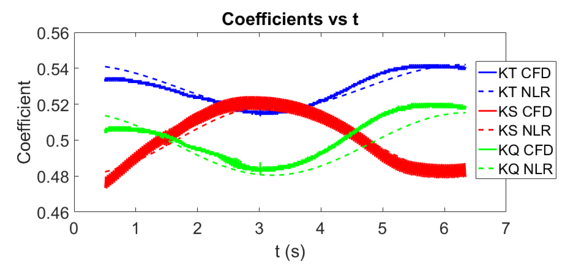
Figure 17 shows the coefficients predicted by the nonlinear regression compared to those computed from the CFD for Test 1. The average loss function is 3.43 $\times {10}^{-5}$, the average L2 norm error of the $K_T$ is 0.003, the average L2 norm error of the $K_S$ is 0.004, and the average L2 norm error of the $K_Q$ is 0.0067. Figure 18 shows the thrust, side force, and torque as a function of time for the nonlinear regression predictions. These results are very similar and nearly indistinguishable compared to those predicted by the neural network. Therefore, both the nonlinear regression and the neural network do a good job of predicting the forces for this case.

4.2.2. Behind Condition Test 2

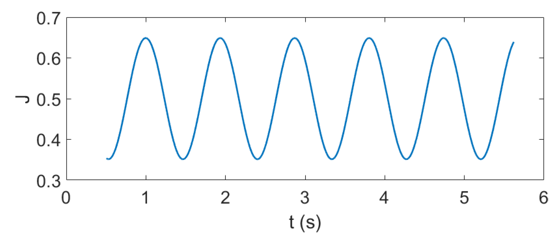
The average forward velocity for Test 2 is reduced to $\overline{U}=1.1$ m/s, the average side velocity is $\overline{V}=0$ m/s, and the average propeller revolution rate is $\overline{n}=20.95$ rev/s. Only the surge degree of freedom is unsteady, with an amplitude of $A_1=0.0487$ m and a frequency of oscillation of ${\omega }_{osc,1}=6.72$ rad/s. This frequency of oscillation was used in [9,17], and it represents the frequency of encounter if the vessel were to be in head seas with the wavelength equal to the length of the waterline. The $\alpha$ is constant at 0 rad. J as a function of time is shown in Figure 19.

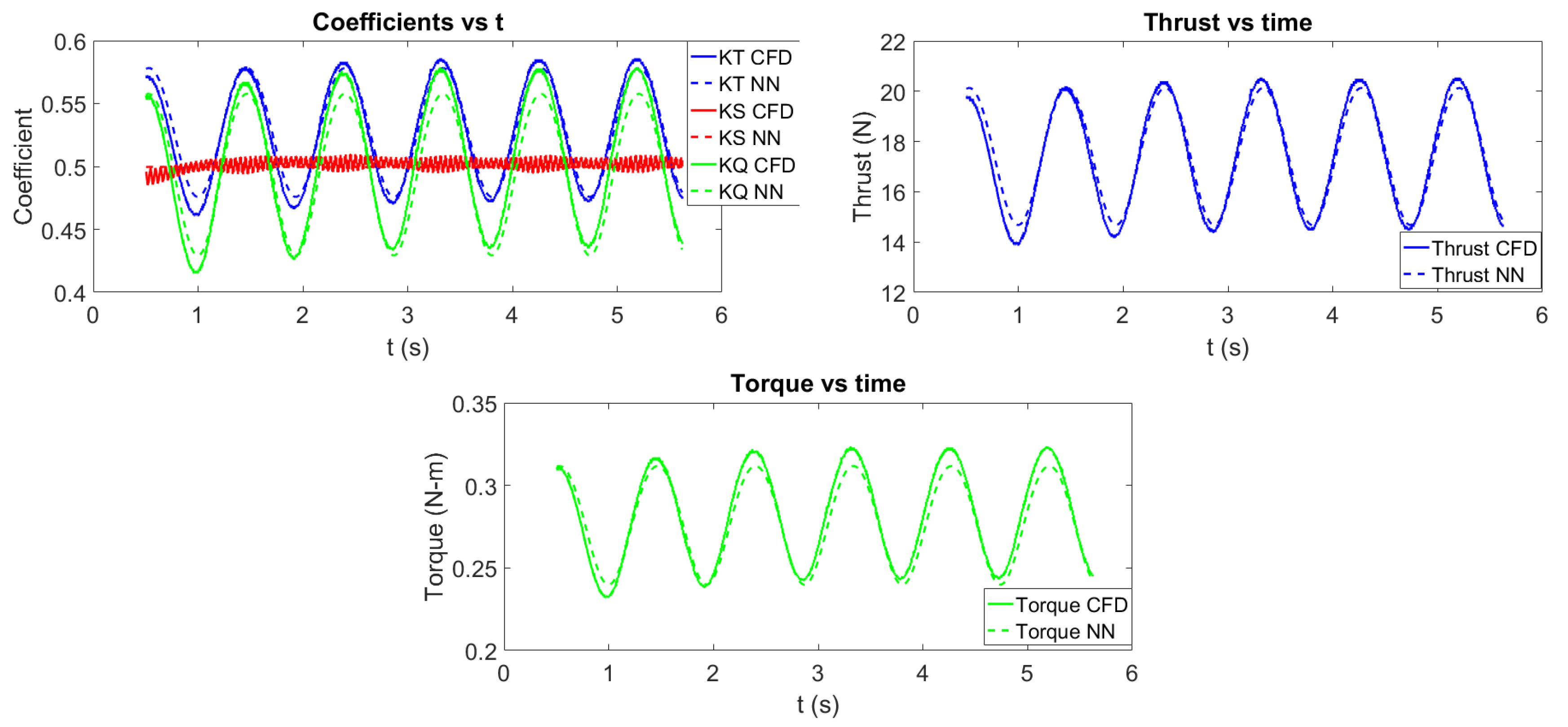
The top left of Figure 20 shows the comparison between the neural network coefficient predictions and the CFD predictions. The average loss function is 1.18 $\times {10}^{-4}$, the average L2 norm error of the $K_T$ is 7.25 $\times {10}^{-3}$, the average L2 norm error of the $K_S$ is 4.58 $\times {10}^{-3}$, and the average L2 norm error of the $K_Q$ is 1.27 $\times {10}^{-2}$. The oscillation in side force is caused by the azimuthal position of the propeller and the resulting force is around zero. The error for $K_T$ and $K_Q$ is higher than Test 1, but still quite accurate. The top right and bottom plots of Figure 20 show the thrust and torque respectively as a function of time. This demonstrates that the neural network can predict the forces well when J oscillates.

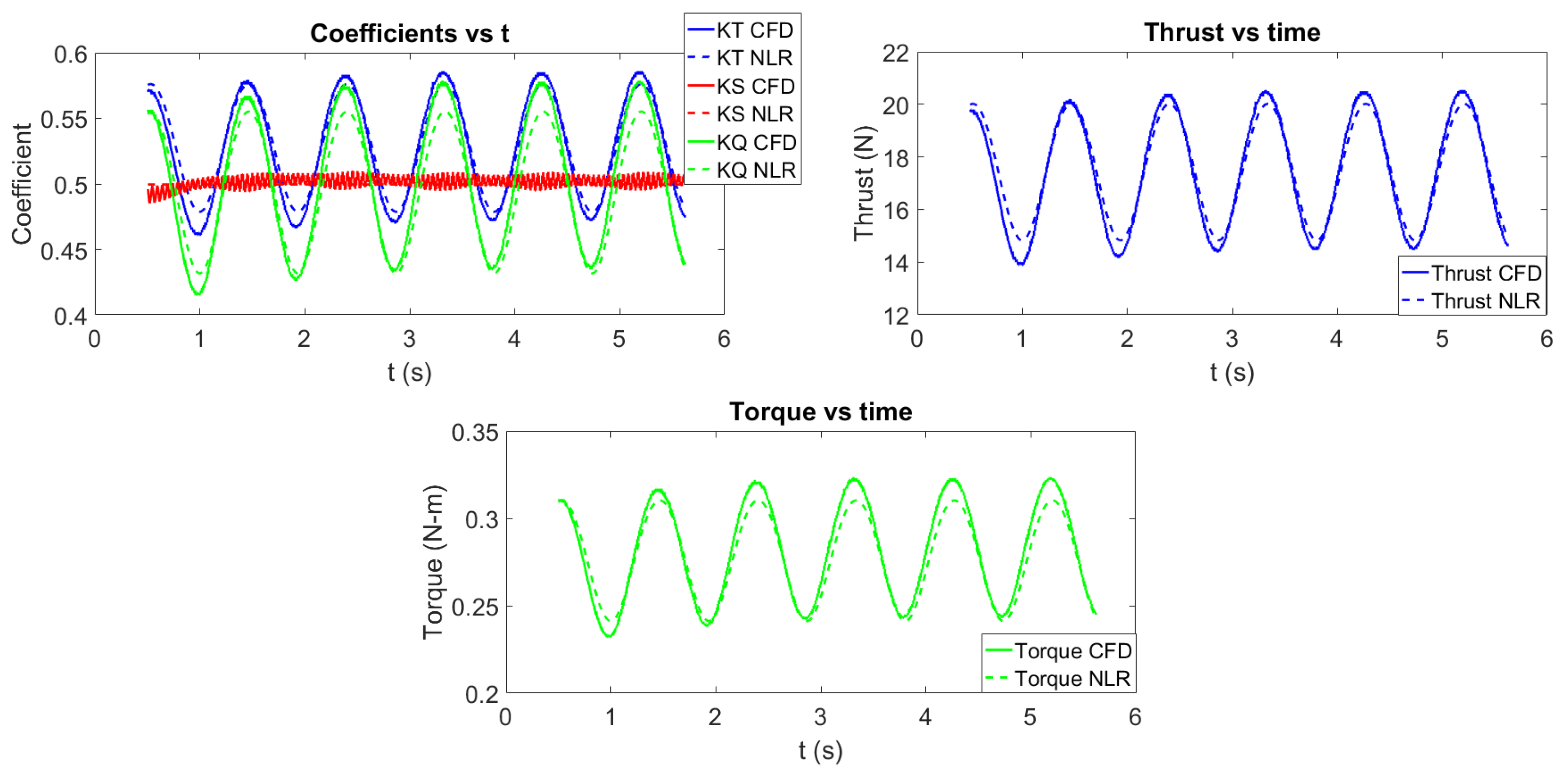
The top left of Figure 21 shows the comparison between the nonlinear regression coefficient predictions and the CFD predictions. The average loss function is 1.18 $\times {10}^{-4}$, the average L2 norm error of the $K_T$ is 8.25 $\times {10}^{-3}$, the average L2 norm error of the $K_S$ is 4.56 $\times {10}^{-3}$, and the average L2 norm error of the $K_Q$ is 1.38 $\times {10}^{-2}$. Thus, the forces are predicted quite similarly to the forces predicted by the neural network. The top right and bottom plots of Figure 21 show the thrust and torque respectively as a function of time.

4.2.3. Behind Condition Test 3

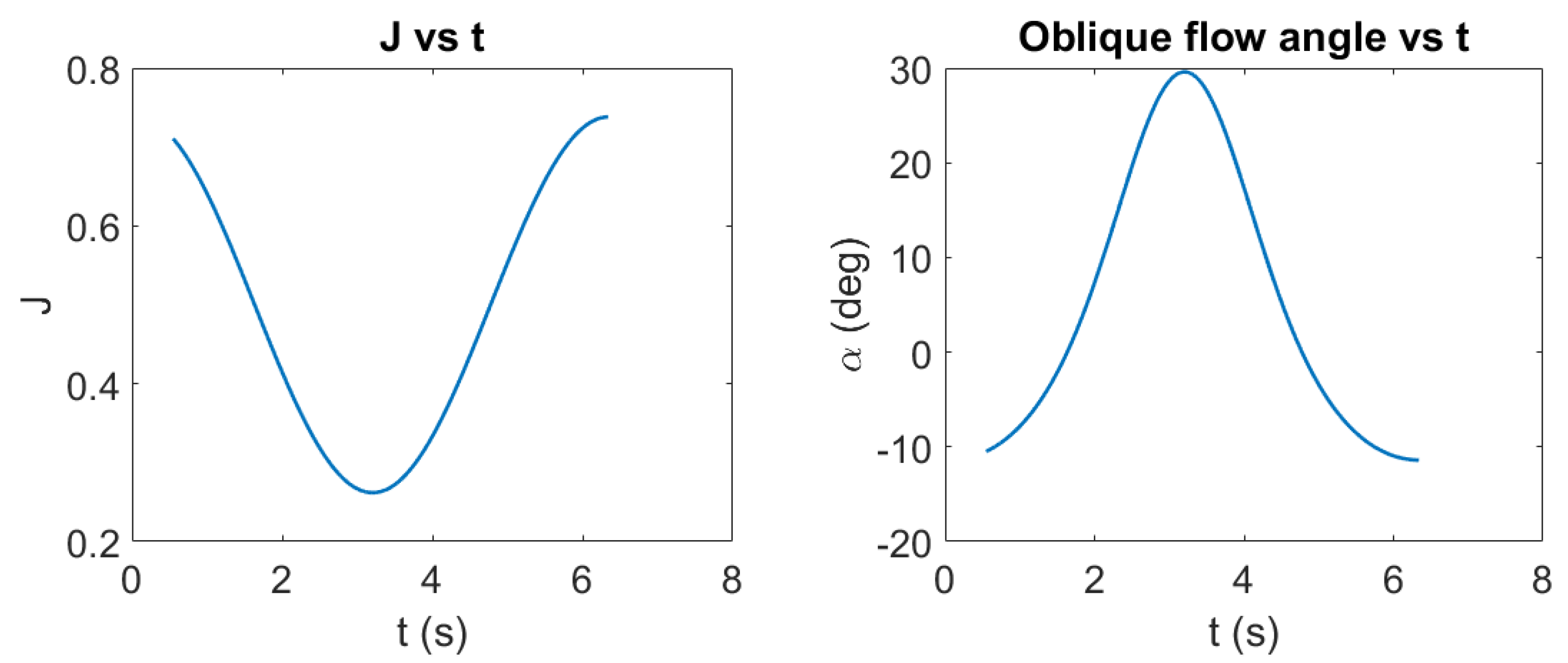
Test three has both unsteady forward velocity as well as unsteady sway velocity. The average forward velocity is $\overline{U}$ = 1.68 m/s, the average side velocity is $\overline{V}$ = 0 m/s, and the average propeller revolution rate is $\overline{n}$ = 32 rev/s. Frequency of oscillation for both surge and sway is ${\omega }_{osc,1}$ = ${\omega }_{osc,2}$ = 1 rad/s. The amplitude of unsteady motion is $A_1$ = 0.8 m and $A_2$ = −0.5 m. Thus, the sway amplitude is larger than the training case and the sway direction is opposite of the Validation case. Figure 22 shows how J and $\alpha$ vary with time for Test 3.

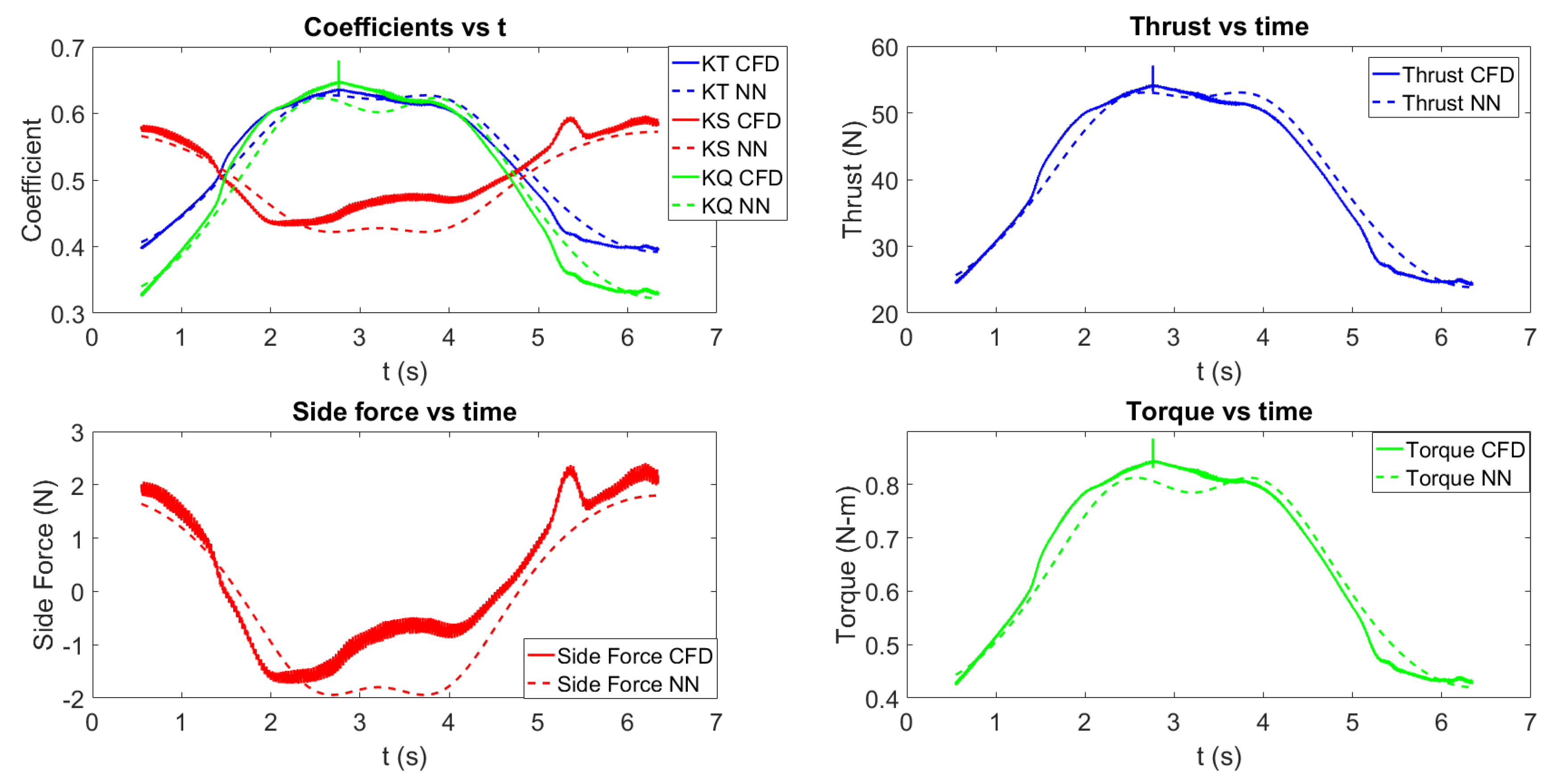
The top left of Figure 23 shows the comparison between the neural network force coefficient predictions and the CFD predictions. The average loss function is 7.30 $\times {10}^{-4}$, the average L2 norm error of the $K_T$ is 1.52 $\times {10}^{-2}$, the average L2 norm error of the $K_S$ is 2.76 $\times {10}^{-2}$, and the average L2 norm error of the $K_Q$ is 2.16 $\times {10}^{-2}$. The top right, bottom left, and bottom right plots of Figure 23 show the thrust, side force, and torque, respectively, as a function of time predicted by the neural network. Overall, good agreement is seen between the CFD and the neural network prediction. The largest error occurs in the prediction of the side force between three and four seconds when the J is low and the oblique flow angle is large.

The top left of Figure 24 shows the comparison between the nonlinear regression force coefficient predictions and the CFD predictions. The average loss function is 2.66 $\times {10}^{-3}$, the average L2 norm error of the $K_T$ is 4.32 $\times {10}^{-2}$, the average L2 norm error of the $K_S$ is 1.72 $\times {10}^{-2}$, and the average L2 norm error of the $K_Q$ is 5.63 $\times {10}^{-2}$. Thus, the forces predicted by the nonlinear regression method are not as accurate as those predicted by the neural network in terms of the L, $K_T$, and $K_Q$. However, the regression model does outperform the $K_S$ neural network prediction. The top right, bottom left, and bottom right plots of Figure 24 show the thrust, side force, and torque, respectively, as a function of time.

5. Conclusions

A neural network and a nonlinear regression model have been trained and tested to determine the unsteady propeller forces due to unsteady motions. The first neural network examined is for open water and it takes a feature vector comprised of various permutations of the instantaneous J and $\left|\alpha \right|$ for each instant in time. A second-order nonlinear regression model was also trained using the instantaneous J and $\left|\alpha \right|$ for each instant in time. The models are extended to the behind condition. The neural network for the behind condition used a similar feature vector, but with the difference of using $\alpha$ instead of $\left|\alpha \right|$. An early stopping procedure is used for the neural network to avoid overtraining. Different feature vectors are examined for the behind condition nonlinear regression, but the second order regression model is shown to be more accurate than higher order regression models that overfit the training data. Both the neural network and the regression approaches are able to predict the unsteady propeller forces for unsteady motions, but the neural network is more accurate for the cases examined. This study is a demonstration of how a neural network and nonlinear regression model can be trained and tested to predict the correct propeller forces for unsteady motion.

The behind condition models could be further improved by incorporating other features in the input. For example, the feature vector could be expanded to incorporate history terms to account for memory effects in the flow. Furthermore, probes could be placed upstream of the propeller plane and the effects of shed vortices from the hull or incident velocities could be accounted for.

The regression model could be improved by supplying additional training to the model. Latin hyper cube sampling could be used to generate training data to cover the full J-$\alpha$ space. However, additional training would clearly lead to increased training cost. Thus, for the cases examined, as the neural network tends to be more accurate than the nonlinear regression, it may be preferable since it can be more accurate than the regression model with limited training.

The models, especially the behind condition neural network, could be very useful for analyzing a maneuvering vessel. Instead of having to discretize the propeller and use a rotating mesh to simulate the viscous effects on the propeller, the neural network or regression model could be used. This could dramatically reduce the cost of a maneuvering calculation using CFD. Furthermore, the models could be trained with any type of training data whether it be experiments, potential flow calculations, RANS CFD, LES, or any combination of these. For example, LES could be used to train the neural network in off design circumstances and potential flow methods could be used to train the on design points.

References

- Carrica, P.M.; Sadat-Hosseini, H.; Stern, F. CFD analysis of broaching for a model surface combatant with explicit simulation of moving rudders and rotating propellers. Comput. Fluids 2012, 53, 117–132. [Google Scholar] [CrossRef]
- Mizzi, K.; Demirel, Y.K.; Banks, C.; Turan, O.; Kaklis, P.; Atlar, M. Design optimisation of propeller boss cap fins for enhanced propeller performance. Appl. Ocean Res. 2017, 62, 210–222. [Google Scholar] [CrossRef] [Green Version]
- Wang, J.; Zou, L.; Wan, D. Numerical simulations of zigzag maneuver of free runnig ship in waves by RANS-Overset grid method. Ocean Eng. 2018, 162, 55–79. [Google Scholar] [CrossRef]
- Shen, Z.; Wan, D.; Carrica, P.M. Dynamic overset grids in OpenFOAM with application to KCS self-propulsion and maneuvering. Ocean Eng. 2015, 108, 287–306. [Google Scholar] [CrossRef]
- Ortolani, F.; Dubbioso, G.; Muscari, R.; Mauro, S.; Mascio, A.D. Experimental and Numerical Investigation of Propeller Loads in Off-Design Conditions. J. Mar. Sci. Eng. 2018, 6, 45. [Google Scholar] [CrossRef] [Green Version]
- Mousaviraad, S. CFD Prediction of Ship Response to Extreme Wind and/or Waves. Ph.D. Thesis, University of Iowa, Iowa City, IA, USA, 2010. [Google Scholar]
- Yao, J. On the Propeller Effect When Predicting Hydrodynamic Forces for Manoeuvring Using RANS Simulations of Captive Model Tests. Ph.D. Thesis, Technical University of Berlin, Berlin, Germany, 2015. [Google Scholar]
- Gaggero, S.; Dubbioso, G.; Villa, D.; Muscari, R.; Viviani, M. Propeller modeling approaches for off-design operative conditions. Ocean Eng. 2019, 178, 283–305. [Google Scholar] [CrossRef]
- Knight, B.; Maki, K. A Semi-Empirical Multi-Degree of Freedom Body Force Propeller Model. Ocean Eng. 2019, 178, 270–282. [Google Scholar] [CrossRef]
- White, P.F.; Knight, B.G.; Filip, G.P.; Maki, K.J. Numerical Simulations of the Duisburg Test Case Hull Maneuvering in Waves. In SNAME Maritime Convention; The Society of Naval Architects and Marine Engineers: Tacoma, WA, USA, 2019. [Google Scholar]
- Broglia, R.; Dubbioso, G.; Durante, D.; Mascio, A.D. Simulation of turning circle by CFD: Analysis of different propeller models and their effect on manoevring prediction. Appl. Ocean Res. 2013, 39, 1–10. [Google Scholar] [CrossRef]
- Phillips, A.; Turnock, S.; Furlong. Evaluation of manoeuvring coefficient of a self-propelled ship using blade element momentum propeller model coupled to a Reynolds averaged Navier–Stokes flow solver. Ocean Eng. 2009, 36, 1217–1225. [Google Scholar] [CrossRef] [Green Version]
- Winden, B. Powering Performance of a Self Propelled Ship in Waves. Ph.D. Thesis, University of Southampton, Southamptom, UK, 2014. [Google Scholar]
- Hornik, K.; Stinchcombe, M.; White, H. Multilayer feedforward networks are universal approximators. Neural Netw. 1989, 2, 359–366. [Google Scholar] [CrossRef]
- Singh, A.P.; Medida, S.; Duraisamy, K. Machine-Learning-Augmented Predictive Modeling of Turbulent Separated Flows over Airfoils. AIAA J. 2017, 55, 2215–2227. [Google Scholar] [CrossRef]
- Abramowski, T. Prediction of Propeller Forces During Ship Maneuvering. J. Theor. Appl. Mech. 2005, 43, 157–178. [Google Scholar]
- Knight, B.; Maki, K. Body Force Propeller Model for Unsteady Surge Motion. In Proceedings of the ASME 37th International Conference on Ocean Offshore and Arctic Engineering (OMAE), Madrid, Spain, 17–22 June 2018. [Google Scholar]
- Knight, B.; Maki, K. A Data-Driven Multi-Degree of Freedom Body Force Propeller Model for Maneuvering. In Proceedings of the Sixth International Conference on Marine Propulsors (SMP 19), Rome, Italy, 26–30 May 2019. [Google Scholar]
- ITTC. ITTC-Recommended Procedures and Guidelines. 1978 ITTC Performance Prediction Method. International Towing Tank Conference, 2011, 7.5-02, 03-01.4. pp. 1–9. Available online: https://ittc.info/media/8372/index.pdf (accessed on 2 February 2020).
- Seber, G.A.F.; Wild, C.J. Nonlinear Regression; Wiley-Interscience: Hoboken, NJ, USA, 2003. [Google Scholar]
Figure 1.
Schematic of neural network with single hidden layer.
Figure 2.
Discrete samples of J (left) and (right) as a function of time for the unsteady open water propeller training case.
Figure 3.
L as a function of training iteration for the open water neural network.
Figure 4.
Coefficients as a function of time for open water training using the neural network.
Figure 5.
Coefficients as a function of time for the entire time series used for open water training. Seventy snapshots of this series were used to train the neural network.
Figure 6.
Coefficients as a function of time for open water training using nonlinear regression. (Left) Nonlinear regression using a first order feature vector. (Right) Nonlinear regression using the second order feature vector.
Figure 7.
J and as a function of time for the unsteady open water propeller test case.
Figure 8.
Open water coefficients for the test data set comparing CFD to the neural network.
Figure 9.
Open water thrust, side force, and torque for the test data set as a function of time comparing CFD to the neural network.
Figure 10.
Open water thrust, side force, and torque for the test data set as a function of time using nonlinear regression.
Figure 11.
-J space for training, validation, and test cases.
Figure 12.
Coefficients, thrust, side force, and torque for behind condition neural network validation case. Top row: highest tolerance for L. Bottom row: lowest tolerance for L examined.
Figure 13.
Coefficients for the behind condition training cases. Left: Unsteady training. Right: Steady training.
Figure 14.
Coefficients, thrust, side force, and torque for behind condition nonlinear regression validation case. Top row: Lowest order regression. Bottom row: Highest order regression.
Figure 15.
Behind condition Test 1 coefficients as a function of time predicted by neural network.
Figure 16.
Behind condition neural network predictions of thrust, side force, and torque for Test 1 as a function of time.
Figure 17.
Behind condition Test 1 coefficients as a function of time predicted by nonlinear regression.
Figure 18.
Behind condition nonlinear regression predictions of thrust, side force, and torque for Test 1 as a function of time.
Figure 19.
J as a function of time for behind condition Test 2.
Figure 20.
Behind condition coefficients, thrust, and torque for Test 2 as a function of time predicted by the neural network.
Figure 21.
Behind condition coefficients, thrust, and torque for Test 2 as a function of time predicted by nonlinear regression.
Figure 22.
J (left) and (right) as a function of time for Test 3.
Figure 23.
Behind condition coefficients, thrust, and torque for Test 3 as a function of time predicted by the neural network.
Figure 24.
Behind condition coefficients, thrust, and torque for Test 3 as a function of time predicted by nonlinear regression.