Effect of Breaking Waves on Near-Surface Mixing in an Ocean-Wave Coupling System under Calm Wind Conditions


Department of Earth and Marine Science, College of Ocean Sciences, Jeju National University, Jeju 63243, Korea
*
Author to whom correspondence should be addressed.
J. Mar. Sci. Eng. 2020, 8(7), 540; https://doi.org/10.3390/jmse8070540
Submission received: 23 June 2020
/
Revised: 17 July 2020
/
Accepted: 17 July 2020
/
Published: 20 July 2020
(This article belongs to the Special Issue Numerical Models in Coastal Hazards and Coastal Environment)
Abstract
:Estimating wave effects on vertical mixing is a necessary step toward improving the accuracy and reliability of upper-ocean forecasts. In this study, we evaluate the wave effects on upper-ocean mixing in the northern East China Sea in summer by analyzing the results of comparative experiments: a stand-alone ocean model as a control run and two ocean–wave coupled models that include the effect of the breaking waves (BW) and of the wave–current interaction (WCI) with a vortex-force formalism. The comparison exhibits that under weak wind conditions, the BW effect prescribed by wave dissipation energy significantly enhances near-surface mixing because of increased downward turbulent kinetic energy (TKE), whereas the WCI has little effect on vertical mixing. Increased TKE results in a mixed-layer depth deepened by ~46% relative to the control run, which provides better agreement with the observed surface thermal structure. An additional experiment with local wind–based BW parameterization confirms the importance of nonlocally generated waves that propagated into the study area upon near-surface mixing. This suggests that under calm wind conditions, waves propagated over distances can largely affect surface vertical mixing; thus, ocean–wave coupling is capable of improving the surface thermal structure.
1. Introduction
Vertical mixing in the upper-ocean in mid-latitude is one of the main processes in heat transfer between the warm surface layer and the cold subsurface layer, and it greatly influences the ocean–atmospheric interaction through changes in sea surface temperature. Generally, vertical mixing is caused by turbulence that can be generated by many processes, such as winds, tides, and waves, and their interactions [1,2]. Ocean waves influence turbulence generation at the ocean–atmosphere interface and modify the surface boundary layer, thereby affecting vertical mixing in the upper ocean. Over the past few decades, many studies have been carried out to represent ocean–wave mixing in an ocean circulation model using subgrid scale parameterizations [3,4,5]. However, because of the range of scales and processes, it is still limiting and challenging to properly represent wave-induced dynamics in ocean modeling. Studies have pointed out the importance of surface waves in upper-ocean mixing and the need for an ocean–wave coupled modeling system that represents the interaction processes [6,7,8,9,10,11,12,13].
The wave effect on vertical mixing can be presented as an increase in turbulent flow at the boundary layer because of the increase in vertical shear instability generated by wave-induced Stokes drift, i.e., wave–current interaction (WCI) [14,15,16,17], and strengthening of turbulent kinetic energy (TKE) by transferring wave dissipation energy, i.e., breaking waves (BW) [5,18,19]. The changes in the wave-induced current, e.g., Stokes drift and wave-related transport, result in large, vertical eddy diffusivity and thus can play a key role in momentum exchange and vertical mixing [16]. Chune and Aouf (2018) [17] investigated the effect of WCI on the tracer in an ocean circulation model and demonstrated that a warm-biased surface temperature in the tropical ocean can be significantly improved by providing more realistic momentum and energy flux from the wave model.
BW are the principal source of TKE and inject wave energy into the water column, resulting in a near-surface turbulent boundary layer at which energy is dissipated by turbulence [18,20,21]. Wada et al. (2009) [12] showed that wave energy dissipation by BW dominated strong vertical mixing in the continental shelf under strong wind events. Carniel et al. (2009) [22] incorporated the injection of TKE by BW into an ocean model by parameterizing vertical mixing using a generic length scale (GLS) scheme and highlighted the need for wave-induced turbulence to improve the accuracy of temperature structures in the ocean surface.
Our study area in the northern East China Sea (ECS) is mostly characterized by a shallow continental shelf, tides, and monsoonal winds. In summer, surface heating and weak monsoons allow strong stratification, resulting in a vertical thermal structure above the thermocline. This region was widely influenced by the Tsushima Warm Current, which is a branch of Kuroshio in the ECS. The Tsushima Warm Current flows northeastward along the ECS continental shelf and a part of the current enters the Jeju Strait by turning clockwise and then flows eastward. This current is called the Cheju Warm Current [23,24]. The surface thermal structure in the ECS can also be influenced by nonlocally generated waves or swell propagated from the northwestern Pacific Ocean. Using a wave-circulation coupled model, Yang et al. (2004) [25] reported that enhanced vertical mixing by non-BW can improve the thermal structure in the upper 50 m in the northern ECS during summer. However, a warm bias remained near the surface in their model [26], indicating that heat transfer between the warm surface and the cold subsurface water was not sufficient to make the surface mixed-layer depth (MLD) as thick as that observed. Because BW and the WCI can affect the shallow mixed layer within a few meters from the sea surface, understanding of their effect on surface mixing is essential to improving the accuracy of the vertical thermal structure and associated MLD. Nevertheless, less attention has been given to the effect of surface gravity waves on the thermal structure in the ECS, particularly during summer when wind conditions are calm.
In this paper, we evaluate wave effects on surface thermal mixing in the northern ECS during summer using an ocean–wave coupled modeling system. In situ measurement data are compared with the coupled model simulations that include the effects of BW and the WCI. This study also highlights the contribution of nonlocally generated waves to surface thermal mixing by comparing a coupled model simulation with an uncoupled ocean model that includes local wind-based BW parameterization.
2. Modeling System
2.1. Model Configurations
To investigate the effect of waves on surface thermal mixing, we used the coupled ocean–atmosphere–wave–sediment transport modeling system [27]. In this study, the modeling system was composed of an ocean circulation model (regional ocean modeling system, ROMS, https://www.myroms.org/) and a wave model (simulating waves nearshore, SWAN, http://swanmodel.sourceforge.net/).
ROMS integrates the Navier–Stokes governing equation based on the hydrostatic and Boussinesq approximation and is extensively used for various regional and basin-scale modeling studies. To simulate realistic ocean circulation, we used the analysis results of the global hybrid coordinate ocean model as the initial and boundary conditions for sea level, water temperature, salinity, and ocean currents. The 10 tidal constituents (M2, S2, N2, K2, K1, O1, P1, Q1, Mf, and Mm) from TPXO 7 (TOPEX/POSEIDON, https://sealevel.jpl.nasa.gov/missions/topex/) data were imposed to generate the tidal currents and sea-level variations [28]. The surface forcing provided by the National Centers for Environmental Prediction (NCEP) global forecast system (GFS) final analysis data (FNL) with a 1-h interval was used to compute the surface boundary conditions with a bulk formula [29]. The GLS vertical mixing closure scheme using the method was adopted as a vertical mixing parameterization [30,31].
The surface wave simulations were carried out using SWAN, a state-of-the-art, third-generation spectral wave model that computes wind-generated waves in offshore and coastal areas [32]. The model solves the wave action balance equation, which describes the generation, propagation, and dissipation of surface waves. The dissipation of wave energy in the governing equation is represented by the total sum of the whitecapping, bottom friction, and depth-induced breaking terms [33,34]. Whitecapping, which represents wave steepness-related breaking, and wave growth by the surface wind, was calculated based on Komen et al. (1984) [35] and Hasselmann (1974) [36] with default coefficients of SWAN version 41.01. Information about the global wave field from Wave Watch 3 [37] was adopted as the boundary condition to impose the incoming waves propagated into the model domain. We used the wind speed at a 10 m height from the GFS analysis data, the same wind field used as the surface boundary condition of the ocean model, to apply the energy transfer of wind to the wave growth.
Model domains of the ocean and wave models cover the ECS and the Yellow Sea from 22.5° N to 42.5° N and from 113° E to 133° E (Figure 1). The horizontal resolution was set to 1/12° for both the ocean and the wave model. The realistic bathymetry used in the ocean and wave models was extracted from the General Bathymetric Chart of the Oceans (GEBCO), which has a horizontal resolution of 30 s. The ocean model had 20 layers in the vertical stretched terrain-following coordinate. Both the ocean and the wave model were initialized at 00:00 UTC on 22 June 2017. The models were spun up using their initial states for a week to obtain a stable solution before the analysis on July. Because the initial state of the ocean model was obtained from near-real time, high-resolution, and operational analysis of HYCOM (hybrid coordinate ocean model), a week of spin-up period was known be enough to resolve the steady state in the ocean simulation. A series of comparative experiments were performed during July 2017.
2.2. Experimental Design
Four experiments were designed to investigate the effects of BW and the WCI on surface thermal mixing: (1) a stand-alone ROMS model as a control run, (2) two-way coupled ROMS-SWAN without the WCI effect but including the BW effect (BW run), (3) two-way coupled ROMS-SWAN without the BW effect but including the WCI effect (WCI run), and (4) a stand-alone ROMS model with local wind-based BW parameterization (CB run). The experimental designs are listed in Table 1. In the coupled experiments, the two models were coupled via the Model Coupling Toolkit [38,39], which allowed informational exchange between ROMS and SWAN. In the coupled procedure, ROMS received updated wave information (i.e., wave dissipation energy, significant wave heights, wave periods, and directions) from SWAN. Additionally, ROMS passed the barotropic current field to the governing equation of the SWAN according to the method of Kirby and Chen (1989) [40], sharing sea level variation and bathymetry.
In the BW run, the ocean model estimated the effect of wave breaking on surface thermal mixing using wave dissipation energy directly transferred from the spectral wave model. The dissipated wave energy was converted into TKE in the process of vertical mixing [41], which was determined by the GLS two-equation turbulence model [30,31]. The additional TKE production in the GLS scheme is given by the following:
where is the Schmidt number for the eddy diffusivity of TKE and is the stability coefficient. Both are constant in GLS . The nondimensional parameter is bounded by 0, meaning no contribution of the wave to TKE, and 1, meaning all wave dissipation energy goes to TKE. The surface roughness length that determines the turbulence length scale is calculated by , where is the significant wave height transferred from the wave model [22,42]. The turbulence length scale contributed little to surface mixing in all experiments because of the relatively low height of the waves during the study period (data not shown). Therefore, the BW run allowed the BW effect on thermal mixing through changes of TKE because of wave dissipation energy transferred from the wave model. Unlike in the BW run, in the control and WCI runs, wave dissipation energy that resulted from wave breaking was not considered in TKE production, whereas wind-induced surface stress τ was directly added as follows:
Surface roughness was also parameterized by wind stress, as described in Charnok (1955) [43]. The WCI run computed the wave effects on the oceanic circulation using a vortex-force formalism [44]. This vortex-force method considers the wave-induced current and its mass flux transport, including the Stokes drift, Stokes–Coriolis interaction, pressure gradient modifications because of wave-induced sea-level perturbation, and vortex-force terms [44]. Because wave dissipation energy resulting from BW was not considered in the WCI run, it was expected that the vertical thermal mixing caused by TKE production would be mainly determined by the wave-induced current changes in this experiment.
In the CB run, the BW effect on turbulence was parameterized by the assumption that BW can be described by the surface wind stress τ with a control parameter c [18].
3. Results
3.1. Model Validation
Before analyzing the effects of waves on upper-ocean mixing, we needed to confirm that the wave model yielded acceptable performance. First, the NCEP/FNL wind data used in the numerical experiments were compared with the data measured using the buoy at Mara (Figure 1b), which is the buoy closest to the area of conductivity, temperature, and depth (CTD) observation, from 1 to 30 July 2017.
Overall, a weak wind speed of less than ~10 m/s was measured at the buoy location. The FNL wind matched the buoy observation throughout the study period, with a mean root mean square error of less than 1.72 m/s. This implies that the wind data used in our experiments was reasonable for simulating the wave fields. Weak wind, of less than 5 m/s, was observed during the in situ CTD surveys on 24 July 2017.
Then, the modeled significant wave height was validated by direct observation at the Mara buoy (Figure 2b). The observed wave height was in the range from 0.5 to 2.8 m during the period. In particular, notably weak wave heights of less than 1 m were found on 24 July 2017 during CTD measurement when weak wind conditions prevailed. The wave model (BW run) reproduced the timing and magnitude of the observed significant wave height at the buoy location, with a root mean square error of 0.38 m (red line in Figure 2b). The simulated significant wave height from the WCI run is not shown here, because almost no difference was found between BW and WCI runs. The statistical indices, including bias, root mean square error (RMSE), linear correlation coefficient, and the index of agreement (IOA, Willmot et al. 2012 [46]) of wind forcing and modeled , are provided in Table 2.
The vertical temperature structure measured along the CTD stations shown by Figure 1b was compared to validate the ocean model result with respect to the upper-ocean’s thermal structure. The vertical structures of temperature along each line on 24 July 2017 obtained from the observation and control experiments are shown in Figure 3. For all lines, the observations showed that the water columns in July were well stratified, with a strong thermocline at a 10 to 20 m depth, and that the thermoclines gradually sloped downward from offshore toward shore (A1, B1, and C1 stations) because of strong tidal mixing near the western coast of Jeju Island. Below the thermocline, offshore cold water existed that originated from Yellow Sea’s bottom cold water [24,47]. Of particular interest is that above the thermocline, the water column was well mixed for all lines, despite weak wind conditions of less than 5 m/s, with the surface MLD reaching a depth of about 6–12 m. The ocean model from the control run captured the general features of the observed temperature structures along the vertical sections. The strong surface stratification with cold bottom water of ~125° E appeared in all sections, showing a downward slope of the thermocline to the shore, which was fairly consistent with the observed distribution. However, in the surface layer, vertical mixing was weaker compared with the observation, showing a shallow MLD of ~2.5 m, which corresponds to less than half of the observed MLD. This result indicates that the vertical mixing process of the surface layer needs to be improved in the ocean circulation model and that surface gravity waves may be a factor for improvement of the surface mixing effect.
3.2. Effect of Waves on the Ocean-Surface’s Thermal Structure
To examine wave-induced changes in the vertical structure of water temperature, we analyzed the differences between the control run and the three other experiments (Figure 4). The largest effect on the thermal structure was found in the result from the BW run that used an ocean–wave coupled system (Figure 4a–c). In all transects, strong negative temperature differences were clearly confined to a thin surface layer, shallower than ~3 m, which corresponds to the MLD calculated from the control run. Below the surface layer, the water became warmer, with the maximum temperature difference at a depth of about 5–8 m. These changes in the vertical thermal structure imply a decrease in stratification near the surface layer. The effect of wave breaking was also evident from the vertical profiles of the section-averaged temperature difference between the control run and the three other runs (Figure 5). The BW run yielded the most remarkable thermal changes in the near-surface layer, resulting in an increase of ~46% in MLD compared with that of the control run. Although the BW run still underestimated the observed MLD, it provided better agreement with the observation. However, different responses of vertical temperature were found in the results of the WCI run (Figure 4d–f). The WCI with a vortex-force formalism affected the thermal structures mainly below the near surface, showing different responses in each section. The temperature changed through the water column below the surface layer, particularly near the shore where the tidal currents are relatively strong. It is likely that the temperature was horizontally redistributed because of changes in ocean current through the WCI. However, unlike the BW run, little effect occurred in the surface layer for all sections (Figure 5), showing no improvement of the MLD. These results demonstrate that the surface temperature decreases while the subsurface layer increases when the BW effect is included in the ocean–wave coupled model, suggesting the surface warm temperature is vertically redistributed.
In an ocean circulation model, the contribution of wave breaking to surface mixing can be parameterized as a function of local wind stress magnitude , as shown in Equation (3) [18,44]. The CB run that is a stand-alone ocean model with BW parameterization reproduced a pattern of vertical temperature differences similar to those of the BW run (Figure 4g–i). The temperature in all sections showed a decrease near the surface and an increase beneath, i.e., a weakened stratification in the near-surface layer. This indicates that the surface thermal structure can be improved by the wave effect parameterized by local wind–based BW in the ocean circulation model. However, as revealed by section-averaged temperature profiles in Figure 5, the changes of vertical temperature in the parameterization were relatively weak compared with the result of the BW run. A small decrease in water temperature was detected in the surface layer, whereas a small increase was seen in the subsurface layer, which was about half that found in the coupled BW run. The difference in the BW effect between the two experiments (i.e., BW and CB runs) is discussed in the following sections.
4. Discussion
4.1. Surface Thermal Mixing Induced by BW
The preceding model comparisons suggest that under weak wind conditions, BW have the potential to strengthen surface thermal mixing above the thermocline when coupled with the wave model. In an ocean model, the vertical thermal structure is primarily controlled by vertical diffusion in the mixing processes so that the wave effects on vertical mixing can be quantified through vertical diffusion in the ocean model. To examine the contribution of vertical mixing to the surface thermal structure, the vertical diffusion term () in the temperature rate equation on the section along line B was compared in the comparative experiments (Figure 6). Because of weak wind conditions and summer heating, strong vertical mixing was restricted to a surface layer shallower than ~3 m in the control run (Figure 6a), suggesting that without the wave effects, vertical heat exchange is restricted to shallow surface water. However, vertical diffusion reached the top of the thermocline when BW were included in the ocean–wave coupled model, i.e., the BW run (Figure 6b). Comparison between the control run and the BW run indicates that BW can deepen the surface MLD above the thermocline, thereby contributing to surface cooling (Figure 4a–c). The WCI run that included Stokes–Coriolis forcing yielded vertical diffusion similar to that of the control run (Figure 6c) and consequently contributed little to the surface thermal structure (Figure 4d–f). Meanwhile, BW parameterized by local wind stress (i.e., the CB run) affected vertical diffusion in the surface layer but were not significant compared with the BW run.
Vertical mixing in the ocean model is determined by TKE and the turbulent length scale in the GLS turbulence closure [30,31]. To identify the wave effects on TKE near the surface, the vertical TKE profiles obtained from the comparative experiments were compared on line B (Figure 7a). In the control run (black solid line), the highest TKE was found in the surface layer and its value sharply decreased down to an ~4 m depth, but it remained constant beneath this depth. With wave-breaking turbulence, i.e., the BW run, the maximum value of TKE was ~ m2/s2 in the surface layer, which is 10 times greater than that of the control run. TKE transferred downward sharply decreased with depth to ~ m2/s2 at a depth of ~6 m, which was deeper than that of the control run. At the same time, the increased and deepened TKE in the surface layer resulted in increases in vertical eddy viscosity and diffusivity, as shown in Figure 7b,c, respectively. Unlike the BW run, TKE and the associated vertical viscosity and diffusivity profiles obtained from the WCI run (blue line) show almost the same responses as those of the control run, suggesting that the wave-induced current changes have little effect on TKE intensification.
TKE responses to wave forcing are clearly evident in Figure 8, which shows the temporal changes of the TKE profile averaged on line B from the comparative experiments. In the control and WCI runs, TKE (Figure 8a,c), restricted to the shallow surface layer, rapidly intrudes down to a depth of ~15 m on 26–27 July 2017 and then rises suddenly on 29–30 July. These changes in the TKE profile correspond to fluctuations of wind speed measured at the ocean buoy (Figure 2a). For example, the minimum TKE at the surface was found on 28–29 July when the wind speed was the smallest (less than ~2 m/s). This shows that the TKE profile mostly depends on shear production resulting from wind conditions, because there is no TKE injection by waves. However, the BW run produces relatively strong TKE in the surface layer during the period (Figure 8b). In particular, even though the wind was the weakest on 28–29 July, the surface TKE was more than 10 times greater than in the control and WCI runs. These comparisons indicate that under weak wind conditions, wave dissipation energy caused by breaking is a key source of enhanced TKE and consequently affects surface thermal structures through intensified vertical mixing.
4.2. Effect of Swell-Related BW
Similarly to the BW run, the CB run produced enhanced TKE and its temporal changes in the surface layer; however, its magnitude was only about half that observed in the BW run (Figure 7 and Figure 8). As a result, the depth in which TKE intruded downward was shallower in the CB run than in the BW run. Of particular interest is that a pronounced difference between the BW run and the CB run was seen on 28–29 July 2017, when the weakest wind blew. This means that the parameterized BW effect based on the local wind speed has a limitation in terms of producing surface thermal mixing under weak wind conditions.
To gain insight into the role of wave dissipation on surface mixing, we examined the spatial patterns of wind speed and wave heights on 29 July 2017, when the weakest wind blew over the study area (Figure 9). Because of the southerly summer monsoon, relatively strong wind of above ~4 m/s dominates the central ECS region; however, the wind magnitude decreases as it moves north (Figure 9a). In particular, the weakest wind of below ~1.5 m/s appears in the study area, i.e., the western seas of Jeju Island. Because the energy dissipation by wave breaking was parameterized by this local wind speed in the ocean model, the CB run yielded small TKE and associated weak surface thermal mixing in the western seas of Jeju Island. However, during the weak wind period, the surface TKE remained stronger in the BW run, which directly considered wave dissipation energy from the wave model in the ocean–wave coupled system. The horizontal distribution of wave heights from the wave model is roughly associated with the wind pattern but clearly shows northward propagation of high waves from the central ECS toward the study area (Figure 9b). As a result, in the BW run, relatively energetic waves were found in the western seas of Jeju Island which thus resulted in increased TKE because of wave energy dissipation by breaking. This result indicates the importance of nonlocally generated waves or swell on the surface TKE in the study area. The role of waves propagated from the south on the surface TKE is evident in Figure 9c, which shows the contribution of swell, which is independent of local wind, to significant wave height.
Unlike the wind magnitude, the long-period swell accounts for a great portion of the wave heights (~70%) over the study area. Our results suggest that under weak wind conditions, swell propagated over long distances can largely affect surface thermal mixing through wave dissipation energy by breaking; thus, ocean–wave coupling is capable of improving the vertical thermal structure in the near surface, especially in summer.
5. Summary
In situ observations, which were conducted in the northern ECS in summer 2017, showed a well-mixed thermal structure in the near surface, even though local winds are quite weak over the study area. Because waves are among the major sources of the turbulence in the ocean-surface layer that cause vertical thermal mixing, in this study, we examined wave effects on surface thermal mixing in the northern ECS during summer by analyzing the results from a series of numerical experiments. Without wave effects, the ocean model produces a shallow MLD, which corresponds to less than 50% of the observed MLD, indicating insufficient surface thermal mixing. However, the BW effect by wave dissipation energy from the wave model significantly enhances near-surface mixing because of increased downward TKE. Increased TKE results in deepened MLD, by ~46%, relative to the control run, which provides better agreement with the observed surface thermal structure, even though it remains underestimated. This comparison indicates that under weak wind conditions, wave dissipation energy by breaking is a key source of enhanced TKE and consequently affects surface thermal structures through intensified vertical mixing. Unlike wave energy dissipation by breaking, wave-induced currents contribute little to surface thermal mixing, suggesting that the effect of WCI on surface mixing can be ignored in regions where ocean currents and local winds are weak.
In addition, a stand-alone ocean model with local wind-based BW parameterization confirms the importance of nonlocally generated waves on near-surface mixing. Under weak wind conditions, swell propagated over distances significantly affects surface thermal mixing through wave dissipation energy by breaking. This suggests that the ocean–wave coupling model can improve vertical mixing in the surface layer and thus provide a more realistic estimate of the surface thermal structure, especially under calm wind conditions.
Author Contributions
Conceptualization, J.-S.H. and J.-H.M.; methodology, T.K.; validation, J.-S.H.; formal analysis, J.-S.H.; visualization, J.-S.H.; writing—original draft, J.-S.H. and J.-H.M.; writing—review and editing, J.-H.M. and T.K.; supervision, J.-H.M. All authors have read and agreed to the published version of the manuscript.
Funding
This research was supported by the Basic Science Research Program to Research Institute for Basic Science (RIBS) of Jeju National University through the National Research Foundation of Korea (NRF) funded by the Ministry of Education (2019R1A6A1A10072987) and was a part of the Korea Meteorological Administration Research and Development Program under grant KMI2018-07610.
Acknowledgments
The authors would like to thank editor and anonymous reviewers for their insightful comments.
Conflicts of Interest
The authors declare no conflict of interest.
References
- Lim, S.; Jang, C.J.; Park, J. Climatology of the mixed layer depth in the East/Japan Sea. J. Mar. Syst. 2012, 96, 1–14. [Google Scholar] [CrossRef]
- Rimac, A. The Role of Wind Induced Near-Inertial Waves on the Energetics of the Ocean. Ph.D. Thesis, Universität Hamburg, Hamburg, Germany, 2014. [Google Scholar]
- Qiao, F.; Huang, C.J. Comparison between vertical shear mixing and surface wave-induced mixing in the extratropical ocean. J. Geophys. Res. Ocean. 2012, 117. [Google Scholar] [CrossRef]
- Huang, C.J.; Qiao, F.; Shu, Q.; Song, Z. Evaluating austral summer mixed-layer response to surface wave-induced mixing in the Southern Ocean. J. Geophys. Res. Ocean. 2012, 117. [Google Scholar] [CrossRef] [Green Version]
- Wu, L.; Rutgersson, A.; Sahlée, E. Upper-ocean mixing due to surface gravity waves. J. Geophys. Res. Ocean. 2015, 120, 8210–8228. [Google Scholar] [CrossRef] [Green Version]
- Rascle, N.; Ardhuin, F.; Terray, E.A. Drift and mixing under the ocean surface: A coherent one-dimensional description with application to unstratified conditions. J. Geophys. Res. Ocean. 2006, 111. [Google Scholar] [CrossRef] [Green Version]
- Walsh, K.; Govekar, P.; Babanin, A.V.; Ghantous, M.; Spence, P.; Scoccimarro, E. The effect on simulated ocean climate of a parameterization of unbroken wave-induced mixing incorporated into the k-epsilon mixing scheme. J. Adv. Modeling Earth Syst. 2017, 9, 735–758. [Google Scholar] [CrossRef]
- Wang, Y.; Qiao, F.; Fang, G.; Wei, Z. Application of wave-induced vertical mixing to the K profile parameterization scheme. J. Geophys. Res. Ocean. 2010, 115. [Google Scholar] [CrossRef]
- Song, Z.; Qiao, F.; Song, Y. Response of the equatorial basin-wide SST to non-breaking surface wave-induced mixing in a climate model: An amendment to tropical bias. J. Geophys. Res. Ocean. 2012, 117. [Google Scholar] [CrossRef]
- Bruneau, N.; Toumi, R.; Wang, S. Impact of wave whitecapping on land falling tropical cyclones. Sci. Rep. 2018, 8, 1–11. [Google Scholar] [CrossRef] [Green Version]
- Aijaz, S.; Ghantous, M.; Babanin, A.V.; Ginis, I.; Thomas, B.; Wake, G. Nonbreaking wave-induced mixing in upper ocean during tropical cyclones using coupled hurricane-ocean-wave modeling. J. Geophys. Res. Ocean. 2017, 122, 3939–3963. [Google Scholar] [CrossRef] [Green Version]
- Wada, A.; Niino, H.; Nakano, H. Roles of vertical turbulent mixing in the ocean response to Typhoon Rex (1998). J. Oceanogr. 2009, 65, 373–396. [Google Scholar] [CrossRef]
- Lewis, H.W.; Castillo Sanchez, J.M.; Siddorn, J.; King, R.R.; Tonani, M.; Saulter, A.; Sykes, P.; Pequignet, A.-C.; Weedon, G.P.; Palmer, T.; et al. Can wave coupling improve operational regional ocean forecasts for the north-west European Shelf. Ocean Sci. 2019, 15, 669–690. [Google Scholar] [CrossRef] [Green Version]
- Kantha, L.; Lass, H.U.; Prandke, H. A note on Stokes production of turbulence kinetic energy in the oceanic mixed layer: Observations in the Baltic Sea. Ocean Dyn. 2010, 60, 171–180. [Google Scholar] [CrossRef]
- Paskyabi, M.B.; Fer, I.; Jenkins, A.D. Surface gravity wave effects on the upper ocean boundary layer: Modification of a one-dimensional vertical mixing model. Cont. Shelf Res. 2012, 38, 63–78. [Google Scholar] [CrossRef] [Green Version]
- Kumar, N.; Feddersen, F. The effect of Stokes drift and transient rip currents on the inner shelf. Part II: With stratification. J. Phys. Oceanogr. 2017, 47, 243–260. [Google Scholar] [CrossRef]
- Chune, S.L.; Aouf, L. Wave effects in global ocean modeling: Parametrizations vs. forcing from a wave model. Ocean Dyn. 2018, 68, 1739–1758. [Google Scholar] [CrossRef]
- Craig, P.D.; Banner, M.L. Modeling wave-enhanced turbulence in the ocean surface layer. J. Phys. Oceanogr. 1994, 24, 2546–2559. [Google Scholar] [CrossRef] [Green Version]
- Breivik, Ø.; Mogensen, K.; Bidlot, J.R.; Balmaseda, M.A.; Janssen, P.A. Surface wave effects in the NEMO ocean model: Forced and coupled experiments. J. Geophys. Res. Ocean. 2015, 120, 2973–2992. [Google Scholar] [CrossRef] [Green Version]
- Rascle, N.; Chapron, B.; Ardhuin, F.; Soloviev, A. A note on the direct injection of turbulence by breaking waves. Ocean Model. 2013, 70, 145–151. [Google Scholar] [CrossRef] [Green Version]
- Ardhuin, F.; Orfila, A. Wind waves. New Front. Oper. Oceanogr. 2018, 393–422. [Google Scholar] [CrossRef] [Green Version]
- Carniel, S.; Warner, J.C.; Chiggiato, J.; Sclavo, M. Investigating the impact of surface wave breaking on modeling the trajectories of drifters in the northern Adriatic Sea during a wind-storm event. Ocean Model. 2009, 30, 225–239. [Google Scholar] [CrossRef]
- Lie, H.J.; Cho, C.H.; Lee, J.H.; Lee, S.; Tang, Y. Seasonal variation of the Cheju warm current in the northern East China Sea. J. Oceanogr. 2000, 56, 197–211. [Google Scholar] [CrossRef]
- Moon, J.H.; Hirose, N.; Yoon, J.H. Comparison of wind and tidal contributions to seasonal circulation of the Yellow Sea. J. Geophys. Res. Ocean. 2009, 114. [Google Scholar] [CrossRef]
- Yongzeng, Y.; Fangli, Q.; Changshui, X.; Jian, M.; Yeli, Y. Wave-induced mixing in the Yellow Sea. Chin. J. Oceanol. Limnol. 2004, 22, 322–326. [Google Scholar] [CrossRef]
- Huang, D.; Zhang, T.; Zhou, F. Sea-surface temperature fronts in the Yellow and East China Seas from TRMM microwave imager data. Deep Sea Res. Part Ii Top. Stud. Oceanogr. 2010, 57, 1017–1024. [Google Scholar] [CrossRef]
- Warner, J.C.; Armstrong, B.; He, R.; Zambon, J.B. Development of a coupled ocean–atmosphere–wave–sediment transport (COAWST) modeling system. Ocean Model. 2010, 35, 230–244. [Google Scholar] [CrossRef] [Green Version]
- Egbert, G.D.; Erofeeva, S.Y. Efficient inverse modeling of barotropic ocean tides. J. Atmos. Ocean. Technol. 2002, 19, 183–204. [Google Scholar] [CrossRef] [Green Version]
- Fairall, C.W.; Bradley, E.F.; Hare, J.E.; Grachev, A.A.; Edson, J.B. Bulk parameterization of air–sea fluxes: Updates and verification for the COARE algorithm. J. Clim. 2003, 16, 571–591. [Google Scholar] [CrossRef]
- Umlauf, L.; Burchard, H. A generic length-scale equation for geophysical turbulence models. J. Mar. Res. 2003, 61, 235–265. [Google Scholar] [CrossRef]
- Warner, J.C.; Sherwood, C.R.; Arango, H.G.; Signell, R.P. Performance of four turbulence closure models implemented using a generic length scale method. Ocean Model. 2005, 8, 81–113. [Google Scholar] [CrossRef]
- Booij NR, R.C.; Ris, R.C.; Holthuijsen, L.H. A third-generation wave model for coastal regions: 1. Model description and validation. J. Geophys. Res. Ocean. 1999, 104, 7649–7666. [Google Scholar] [CrossRef] [Green Version]
- Madsen, O.S.; Poon, Y.K.; Graber, H.C. Spectral wave attenuation by bottom friction: Theory. In Coastal Engineering 1988; 1989; pp. 492–504. Available online: http://ccrm.vims.edu/yinglong/wiki_files/Manual_SED2D.pdf (accessed on 23 June 2020).
- Battjes, J.A.; Janssen, J.P.F.M. Energy loss and set-up due to breaking of random waves. In Coastal Engineering 1978; 1978; pp. 569–587. Available online: https://icce-ojs-tamu.tdl.org/icce/index.php/icce/article/view/3294 (accessed on 23 June 2020).
- Komen, G.J.; Hasselmann, S.; Hasselmann, K. On the existence of a fully developed wind-sea spectrum. J. Phys. Oceanogr. 1984, 14, 1271–1285. [Google Scholar] [CrossRef]
- Hasselmann, K. On the spectral dissipation of ocean waves due to white capping. Bound. Layer Meteorol. 1974, 6, 107–127. [Google Scholar] [CrossRef]
- Tolman, H.L. A third-generation model for wind waves on slowly varying, unsteady, and inhomogeneous depths and currents. J. Phys. Oceanogr. 1991, 21, 782–797. [Google Scholar] [CrossRef]
- Jacob, R.; Larson, J.; Ong, E. M × N communication and parallel interpolation in Community Climate System Model Version 3 using the model coupling toolkit. Int. J. High Perform. Comput. Appl. 2005, 19, 293–307. [Google Scholar] [CrossRef]
- Larson, J.; Jacob, R.; Ong, E. The model coupling toolkit: A new Fortran90 toolkit for building multiphysics parallel coupled models. Int. J. High Perform. Comput. Appl. 2005, 19, 277–292. [Google Scholar] [CrossRef]
- Kirby, J.T.; Chen, T.M. Surface waves on vertically sheared flows: Approximate dispersion relations. J. Geophys. Res. Ocean. 1989, 94, 1013–1027. [Google Scholar] [CrossRef] [Green Version]
- Moghimi, S.; Thomson, J.; Özkan-Haller, T.; Umlauf, L.; Zippel, S. On the modeling of wave-enhanced turbulence nearshore. Ocean Model. 2016, 103, 118–132. [Google Scholar] [CrossRef] [Green Version]
- Stacey, M.W. Simulation of the wind-forced near-surface circulation in Knight Inlet: A parameterization of the roughness length. J. Phys. Oceanogr. 1999, 29, 1363–1367. [Google Scholar] [CrossRef]
- Charnock, H. Wind stress on a water surface. Q. J. R. Meteorol. Soc. 1955, 81, 639–640. [Google Scholar] [CrossRef]
- Kumar, N.; Voulgaris, G.; Warner, J.C.; Olabarrieta, M. Implementation of the vortex force formalism in the coupled ocean-atmosphere-wave-sediment transport (COAWST) modeling system for inner shelf and surf zone applications. Ocean Model. 2012, 47, 65–95. [Google Scholar] [CrossRef]
- Terray, E.A.; Drennan, W.M.; Donelan, M.A. The vertical structure of shear and dissipation in the ocean surface layer. In The Wind-Driven Air–Sea Interface. Electromagnetic and Acoustic Sensing, Wave Dynamics and Turbulent Fluxes; Banner, M.L., Ed.; School of Mathematics, University of NSW: Sydney, Australia, 1999; pp. 239–245. [Google Scholar]
- Willmott, C.J.; Robeson, S.M.; Matsuura, K. A refined index of model performance. Int. J. Climatol. 2012, 32, 2088–2094. [Google Scholar] [CrossRef]
- Lee, J.H.; Pang, I.C.; Moon, J.H. Contribution of the Yellow Sea bottom cold water to the abnormal cooling of sea surface temperature in the summer of 2011. J. Geophys. Res. Ocean. 2016, 121, 3777–3789. [Google Scholar] [CrossRef]
Figure 1.
(a) Model domain (rotated squared box) and bathymetry (in meters) in the Yellow Sea and East China Sea. The gray box indicates the study area. (b) Stations of in situ conductivity, temperature, and depth (CTD) measurements (black circles) and ocean buoy location (red asterisk). The CTD survey was conducted on 24 July 2017 by the Ocean and Fisheries Research Institute, Jeju Special-Governing Province, Korea.
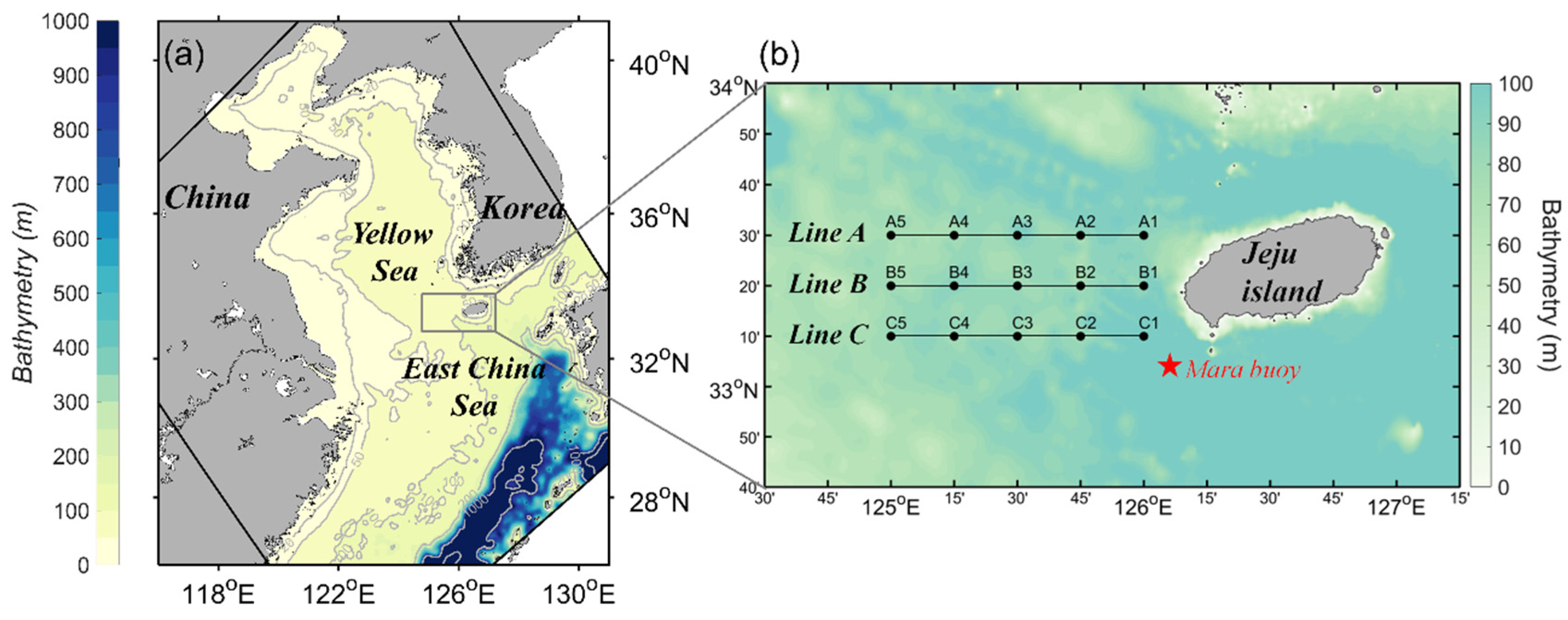
Figure 2.
(a) Time-series comparison of wind speed from FNL (red) and the buoy (black) at the Mara station. (b) Same as (a) except for the significant wave height from the breaking waves (BW) run (red) and the buoy (black) at the Mara station. The shaded period represents the period of CTD observations.

Figure 3.
Vertical sections of temperature from (a–c) the CTD observations and (d–f) the control run along line A (left panels), line B (middle panels), and line C (right panels).
Figure 3.
Vertical sections of temperature from (a–c) the CTD observations and (d–f) the control run along line A (left panels), line B (middle panels), and line C (right panels).

Figure 4.
Vertical sections of temperature differences (a–c) between the BW run and the control run, (d–f) between the WCI run and the control run, and (g–i) between the CB run and the control run along line A (upper panels), line B (middle panels), and line C (bottom panels).
Figure 4.
Vertical sections of temperature differences (a–c) between the BW run and the control run, (d–f) between the WCI run and the control run, and (g–i) between the CB run and the control run along line A (upper panels), line B (middle panels), and line C (bottom panels).
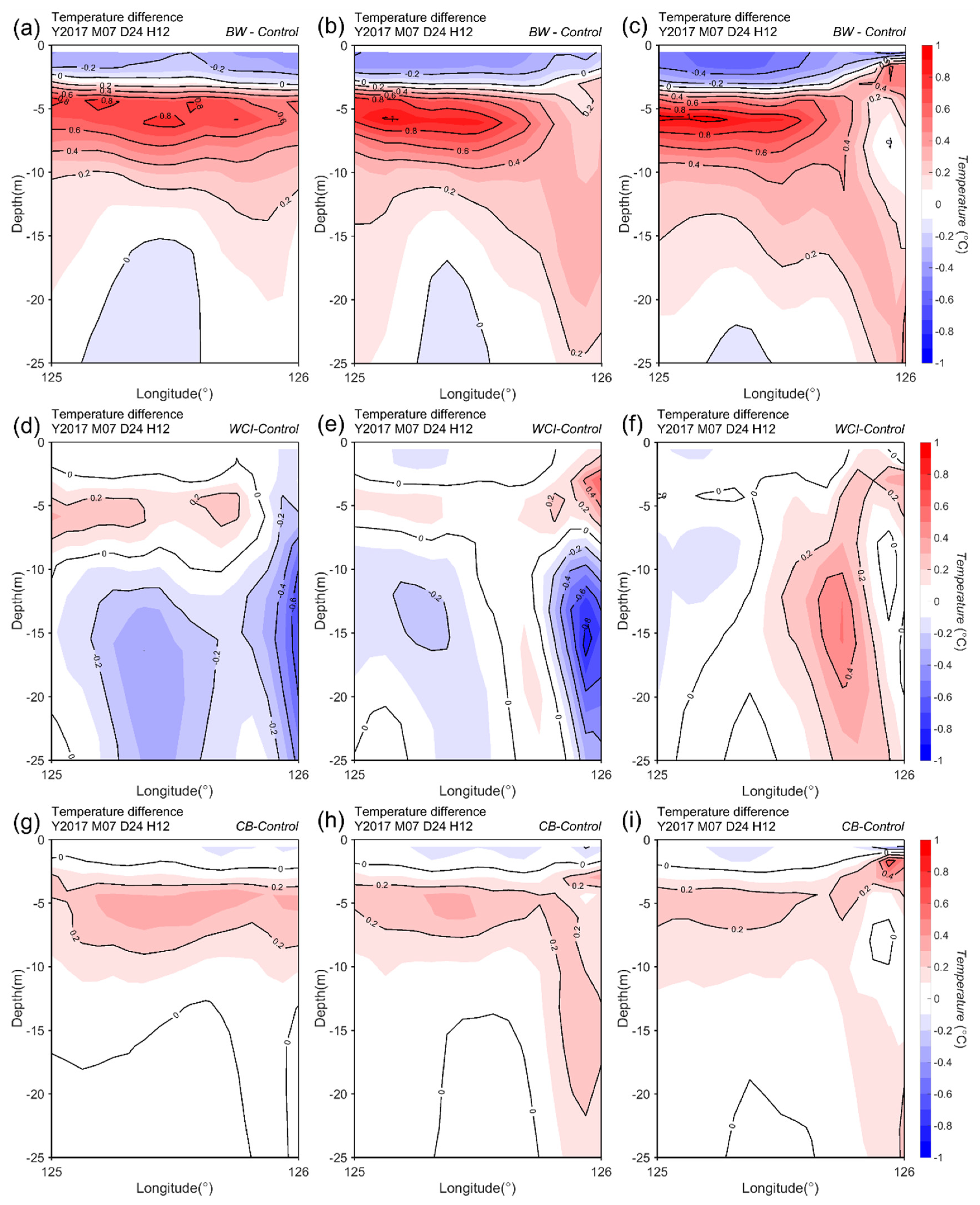
Figure 5.
Vertical profiles of section-averaged temperature differences between each experiment and the control run at (a) line A, (b) line B, and (c) line C on 24 July 2017. Red, blue, and green lines indicate the differences in the BW run, WCI run, and CB run, respectively.
Figure 5.
Vertical profiles of section-averaged temperature differences between each experiment and the control run at (a) line A, (b) line B, and (c) line C on 24 July 2017. Red, blue, and green lines indicate the differences in the BW run, WCI run, and CB run, respectively.

Figure 6.
Vertical sections of the vertical diffusion term (in degrees Celsius per second) in the temperature rate equation obtained from (a) the control run, (b) BW run, (c) WCI run, and (d) CB run along line B on 24 July 2017.
Figure 6.
Vertical sections of the vertical diffusion term (in degrees Celsius per second) in the temperature rate equation obtained from (a) the control run, (b) BW run, (c) WCI run, and (d) CB run along line B on 24 July 2017.

Figure 7.
Vertical profiles of section-averaged (a) TKE, (b) vertical eddy viscosity, and (c) vertical eddy diffusivity in a logarithmic scale at line B on 24 July 2017 obtained from the results of all experiments.
Figure 7.
Vertical profiles of section-averaged (a) TKE, (b) vertical eddy viscosity, and (c) vertical eddy diffusivity in a logarithmic scale at line B on 24 July 2017 obtained from the results of all experiments.
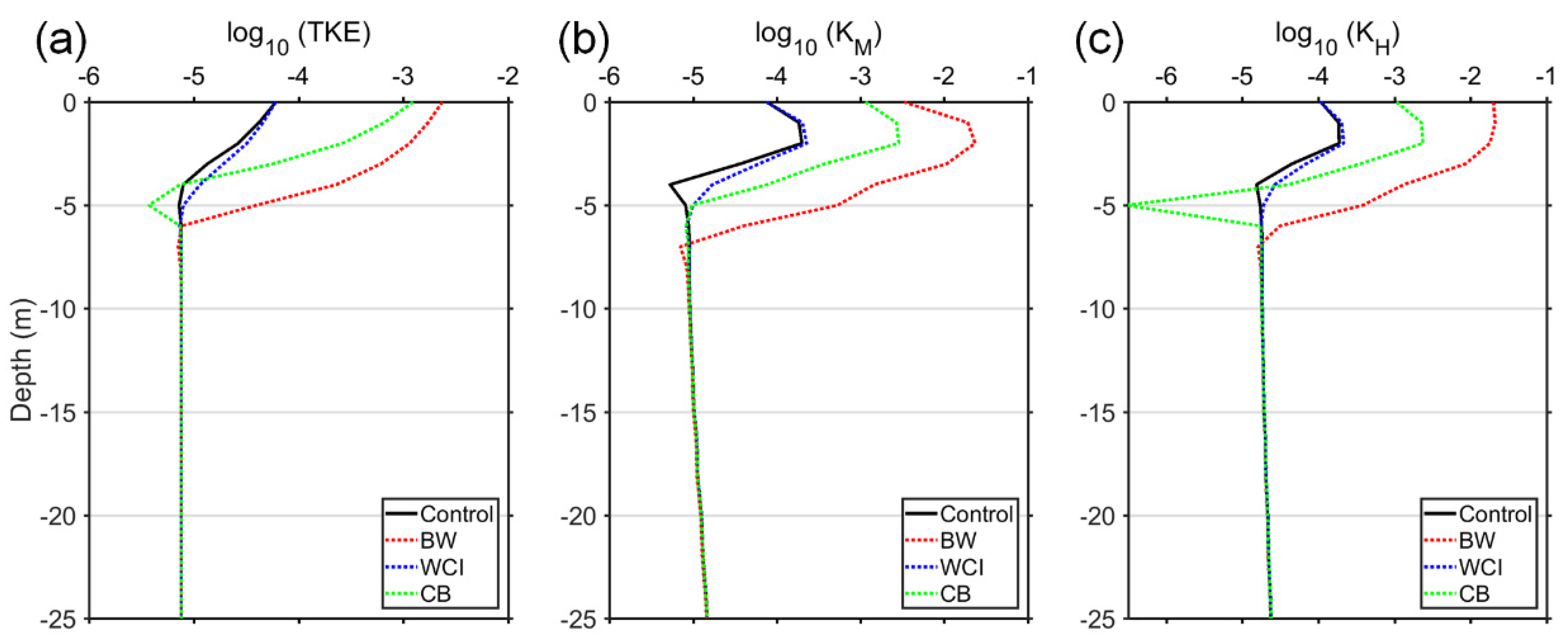
Figure 8.
Depth–time diagram for section-averaged TKE in a logarithmic scale from (a) the control run, (b) BW run, (c) WCI run, and (d) CB run at line B from 22 to 31 July 2017 obtained from the results of all experiments.
Figure 8.
Depth–time diagram for section-averaged TKE in a logarithmic scale from (a) the control run, (b) BW run, (c) WCI run, and (d) CB run at line B from 22 to 31 July 2017 obtained from the results of all experiments.

Figure 9.
Spatial distributions of (a) wind speed at a 10 m height, (b) significant wave height, and (c) the ratio of swell to significant wave height on 29 July 2017 obtained from the wave model in the BW run.
Figure 9.
Spatial distributions of (a) wind speed at a 10 m height, (b) significant wave height, and (c) the ratio of swell to significant wave height on 29 July 2017 obtained from the wave model in the BW run.


Table 1.
Summaries of key processes included in the experiments to introduce wave effects on the near-surface layer.
Table 1.
Summaries of key processes included in the experiments to introduce wave effects on the near-surface layer.
| Wave Effects on the Ocean | Uncoupled | Coupled | ||
|---|---|---|---|---|
| Control | CB | BW | WCI | |
| Breaking wave | Wind-based parameterization (Equation (3)) | Wave dissipation energy ( in Equation (1) from the wave model) | ||
| Wave-Current interaction | Stokes-Coriolis force, Stokes drift advection, Vortex force (Kumar et al. 2012) | |||
Table 2.
Statistics for modeled comparisons with the buoy measurements at the Mara station.
| Bias | RMSE | Correlation | IOA | |
|---|---|---|---|---|
| BW | −0.02 | 0.38 | 0.76 | 0.67 |
| WCI | −0.02 | 0.39 | 0.76 | 0.66 |
© 2020 by the authors. Licensee MDPI, Basel, Switzerland. This article is an open access article distributed under the terms and conditions of the Creative Commons Attribution (CC BY) license (http://creativecommons.org/licenses/by/4.0/).
Share and Cite
MDPI and ACS Style
Hong, J.-S.; Moon, J.-H.; Kim, T. Effect of Breaking Waves on Near-Surface Mixing in an Ocean-Wave Coupling System under Calm Wind Conditions. J. Mar. Sci. Eng. 2020, 8, 540. https://doi.org/10.3390/jmse8070540
AMA Style
Hong J-S, Moon J-H, Kim T. Effect of Breaking Waves on Near-Surface Mixing in an Ocean-Wave Coupling System under Calm Wind Conditions. Journal of Marine Science and Engineering. 2020; 8(7):540. https://doi.org/10.3390/jmse8070540
Chicago/Turabian StyleHong, Ji-Seok, Jae-Hong Moon, and Taekyun Kim. 2020. "Effect of Breaking Waves on Near-Surface Mixing in an Ocean-Wave Coupling System under Calm Wind Conditions" Journal of Marine Science and Engineering 8, no. 7: 540. https://doi.org/10.3390/jmse8070540
Note that from the first issue of 2016, this journal uses article numbers instead of page numbers. See further details here.