
Propulsion Performance and Wake Dynamics of Heaving Foils under Different Waveform Input Perturbations

1
School of Marine Science and Technology, Northwestern Polytechnical University, Xi’an 710072, China
2
Key Laboratory of Unmanned Underwater Vehicle, Northwestern Polytechnical University, Xi’an 710072, China
*
Author to whom correspondence should be addressed.
J. Mar. Sci. Eng. 2021, 9(11), 1271; https://doi.org/10.3390/jmse9111271
Submission received: 27 October 2021
/
Revised: 5 November 2021
/
Accepted: 11 November 2021
/
Published: 15 November 2021
(This article belongs to the Special Issue Computational Fluid Mechanics)
Abstract
:A numerical simulation is used to investigate the effects of adding high frequency and low amplitude perturbations of different waveforms to the sinusoidal-based signal of the heaving foil on the propulsion performance and wake structure. We use the adjustable parameter k to achieve a heaving motion of various waveform cycle trajectories, such as sawtooth, sine, and square. Adding a perturbation of whatever waveform is beneficial in increasing the thrust of the heaving foil, especially by adding a square wave perturbation with a frequency of 10 Hz, pushes the thrust up to 10.49 times that without the perturbation. However, the addition of the perturbation signal brings a reduction in propulsion efficiency, and the larger the perturbation frequency, the lower the efficiency. The wake structure of the heaving foil behaves similarly under different waveform perturbations, all going through some intermediate stages, which eventually evolve into a chaotic wake with the increase in the perturbation frequency. However, a lower frequency square wave perturbation can destabilize the heaving foil wake structure. This work further explains the effect of different waveform perturbation signals on the base sinusoidal signal and provides a new control idea for underwater vehicles.
1. Introduction
Motion is the fundamental property and the existing mode of matter. From running cheetahs to flying swallows and swimming carp, and even to bacteria, moving organisms can be commonly observed. Birds and fish, which usually overcome drag by flapping their wings or fins, can drive themselves with fewer power costs and greater maneuverability after more than 500 million years of natural selection.
Over the past century, researchers have made numerous efforts to learn about the physical mechanisms at the back of flapping propulsion and apply them to bionic vehicles, such as the pioneering work of Garrick [1] and Gray [2], and the theoretical investigations presented by Lighthill [3] and Wu [4]. As the saying goes: three parts land, seven parts ocean. With the over-exploitation of land resources, humans gradually shifted their focus to the ocean, which has more resources, and thus bionic underwater vehicles were born. With the development of technology, scholars have analyzed the skeletal–muscular structure of marine organisms through technical means such as X-ray scanning and dissection, and also used high-speed cameras to photograph the movement of different fishes, summarizing a large number of kinematic equations, which have greatly contributed to the development of bionic vehicles. [5,6,7,8]
Most commonly studied today is the replacement of fins/wings of fish and birds by a simplified model (flapping foil), while simulating biological motion by forcing an excitation signal on the leading edge of the foil. Previously, smooth and periodic excitation signals (sinusoidal, non-sinusoidal, asymmetric functions, etc.) were often chosen to control the foil to accomplish a pure pitch motion, pure heave motion, or a combination of both. Mao et al. [9] used a computational fluid dynamics (CFD) approach to study the hydrodynamic characteristics of 3D flapping foil with different bias angles in pitch motion, and his results can be used to improve control systems for the heave and pitch motions of vehicles. Wu [10] conducted a numerical study on the self-propulsion problem of rigid–flexible composite plates, in which he applied forces to the connection points to keep the rigid part in a given pitch motion, while the deformation of the flexible part was consequent. The effect of the stiffness of the flexible plate was investigated by varying the length ratio of the flexible and rigid parts to simulate the composite plate. In the experiments of Cros [11], a transverse harmonic displacement is applied at the fixed leading edge of the flexible plate. The excitation frequency and air velocity are the two control parameters in their experiment. Their experimental results demonstrate that the resonance phenomenon exhibited by the cantilever plate in the airflow is consistent with the linear theoretical predictions of Eloy [12] and Michelin [13].
However, the simple excitation signals mentioned above cannot accurately represent the mechanisms that generate motor output in biological systems. The reasons for this are mainly the following: Firstly, when fish move, their fins and bodies are deformed, thus generating multiple waves [14,15]. Secondly, the biological locomotor signal is not formed by a single signal, it is generated by a combination of central modulation signals and organ feedback signals [16,17,18]. Finally, the marine environment in which fish live is complex and variable. Therefore, fish must adapt their movements to the changing ocean currents for efficient propulsion. Lehn et al. [19] conducted perturbation experiments in a closed recirculating water tank, where he added a high frequency, low amplitude sinusoidal perturbation signal to the base signal of a sinusoidal heave motion, and the experimental results showed that the addition of the perturbation resulted in a substantial increase in thrust. Inspired by Lehn et al. [19], we add the nonsinusoidal perturbation signal to the sinusoidal base signal and investigate the effects of different waveforms of the perturbation signal on the hydrodynamic characteristics of the heaving foil using numerical simulations.
In this paper, we give the description of the problem and the methodology in Section 2, where the schematic representation of the flow configuration and the kinematics of heaving foil are described. We also define the relevant parameters and validate the numerical method in this section. Then, we discuss the wake structure and hydrodynamics in Section 3. The last section concludes the paper with a summary of our results.
2. Problem Definition and Methodology
2.1. Problem Definition
Figure 1 depicts this problem through a flow schematic. A two-dimensional NACA0012 foil is placed in a uniform flow with constant velocity U in the x-direction. The control signal h(t) consists of the base signal hb(t) and the perturbation signal hp(t). The base signal is a sinusoidal signal, which has a heaving amplitude (A) of 0.25 times the chord length (c) and a fixed frequency (fb) of 1 Hz. The heaving amplitude (0.1 A) of the perturbation signal is 0.025 times the chord length (c) and the frequency (fp) ranges from 0 to 10 Hz with increments of 2 Hz, but its waveform is not fixed, and we will give a detailed definition of the perturbation signal later.
Different from Lehn et al. [19], the adjustable parameter k is used to achieve perturbation signals of various waveform cycle trajectories, such as sawtooth, sine, and square. According to the work of Lu [20], we define the nonsinusoidal heaving perturbation signal of the foil as follows:
where hp(t) denotes the instantaneous heaving perturbation amplitude, hp0 is the maximum heaving amplitude, f is the heaving frequency, and t is the instantaneous time. In Equation (1), we regulate the trajectory of the heaving perturbation signal through an adjustable parameter k. As k increases, the heaving perturbation signal changes from a sawtooth wave to a sine wave and finally to a square wave. In Figure 2, we use the k adopted in this study to show the waveform shapes of various perturbation signals.
We present several dimensionless parameters to describe the motion of the foil. The non-dimensional heave amplitude h, Reynolds number Re, and non-dimensional frequency are defined:
where v is the kinematic viscosity of the fluid, U is the incoming flow velocity, which has been described earlier, A is the heaving amplitude of the base signal, c is the chord length, and here f is the base frequency (fb).
To analyze the forces produced by the heaving foil, we use the symbols CT and CL to represent the instantaneous thrust coefficient and the instantaneous lift coefficient of the heaving foil, respectively. Where s is the span length. Hence, the time-averaged coefficients over a motion period are calculated as:
According to the definition, it can be easily found that produces thrust while produces drag. From the previous study [21], we computed the instantaneous power coefficient, CP, as . Therefore, the time-averaged input power coefficient is calculated as:
Thus, the propulsion efficiency of the heaving foil is determined as:
2.2. Numerical Approach
Numerical simulation of the unsteady flow field around the heaving foil is performed with the software Fluent 20.0. The finite volume method (FVM) is used to discretize the Navier–Stocks equations. The PISO (Pressure-Implicit with Splitting of Operators) algorithm is used to solve the coupled velocity–pressure solution. Momentum discretization is performed using the second-order windward method and derivatives are calculated on the basis of Green-Gauss nodes. The foil motion is achieved by user-defined functions (UDF).
The computational domain consists of two parts: the inner domain and the outer domain. The total size of the computational domain is a rectangle of 20c × 12c, and the inner domain is 10c × 3c. The inner domain uses an unstructured grid to reduce computational resources by the dynamic diffusion grid method and avoid obvious changes in the grid, and the outer domain uses a structured grid.
The boundary conditions of the calculation area are set as follows: the inlet boundary is the velocity inlet; the outlet boundary is the pressure outlet, and the no-slip boundary conditions are used for the foil’s surface and the upper and lower boundaries.
2.3. Validations
To verify the grid-independence, three grid sizes (coarse, medium, and fine) were selected, and the number of grids in grid 1 to 3 was 9 × 10⁴, 2 × 10⁵, and 3 × 10⁵. The CT curves of the heaving foil at h = 0.25, fb = 1 Hz, and fp = 0 Hz were used to verify the grid-independence. The convergence validation of grids 1 to 3 is shown in Figure 3a. There is no significant difference in the CT variation under the three grid scales, indicating that the numerical calculation is grid convergent, and the subsequent results are analyzed using the calculation results of grid 2.
To verify the reliability of the calculation method, the results of this paper are compared with those of Heathcote [22] and Ashraf [23]. Heathcote conducted experiments on a NACA0012 airfoil with an amplitude h = 0.175 at different frequencies . To determine whether turbulence effects play an important role in the flow, Ashraf compared his calculations with the Sparlart–Allmaras turbulence model and the experimental results of Heathcote. It was shown that the NS (Navier-Stokes) laminar simulation results coincided with the turbulence simulation results and were similar to the experimental data when the product of the dimensionless amplitude h and the dimensionless frequency was less than 1.5 (h < 1.5). From Figure 3b, we can see that the calculation results of the method in this paper are in good agreement with the experimental results and are better than the calculation results of Ashraf. A time-step refinement study has also been performed by varying the number of time steps per cycle. For this study, 500, 800, 1000, and 1500 steps were used, using a medium grid for each cycle. As shown in Figure 3c, increasing the resolution of the time step from 1000 to 1500 steps per cycle does not change the thrust coefficient. Therefore, in our study, we use 1000 steps for further simulations.
3. Result and Discussion
To investigate the physical mechanism behind the effect of different waveform perturbation signals on the heaving foil, this section shows the average thrust coefficient, propulsion efficiency, and wake structure of the heaving foil for different waveforms of perturbation signals.
3.1. Force Measurement
From the preceding parameter settings, we can see that the base frequency fb has been kept constant at 1 Hz and the perturbation frequency fp is in variation. Therefore, the calculation period is determined by the base frequency, which means that one calculation period is 1 s and the total calculation time is 10 s. Note that all calculations are averaged over the last two cycles.
The variation of the thrust coefficient of the heaving foil with the perturbation frequency for different waveform perturbations is shown in Figure 4. The comparisons between square and sine, and sawtooth and sine waves are carried out in Figure 4a,b, respectively. The 0 Hz perturbation frequency means that the input signal is only the base signal.
The thrust coefficient of the heaving foil gradually improves as the perturbation frequency increases, which is consistent with the conclusion reached in the experiment of Lehn et al. [19]. We also observe that the sine wave perturbation signal brings a slightly better thrust enhancement than the sawtooth wave, while the square wave perturbation signal brings a substantial thrust enhancement, and we can observe that at k = 5 and fp = 10 Hz, the thrust is directly raised to 1049.89% of that without the addition of perturbation. However, we did not observe the peak thrust as in the experiment of Lehn et al. [19], perhaps because the stiff foil used in his experiment is defined only relative to the flexible foil he used and is not an absolutely rigid body.
For the purpose of quantifying the effect of perturbation frequency on the thrust coefficient, we attempted to fit a response function from the data to derive the corresponding thrust coefficient based on the input perturbation parameters. We fitted a polynomial of the fourth order to the existing thrust coefficient and perturbation frequency curves to obtain the following equation.
where y represents the value of the thrust coefficient and x represents the value of the perturbation frequency. To test the accuracy of the empirical equation we obtained, we numerically simulated that the value of the thrust coefficient under a 12 Hz sinusoidal wave perturbation is 0.9429, which was calculated from our fitted equation as 0.9505, resulting in an error of 0.81%. This indicates that the fitted equation is predictive and yields a universal relationship between the perturbation parameters and the thrust coefficients.
Figure 5 illustrates the variation pattern of propulsion efficiency with perturbation frequency for heaving foil under five perturbation waveforms. As can be seen from the figure, the propulsion efficiency of the heaving foil tends to decrease as the perturbation frequency increases, regardless of which waveform perturbation is added. The propulsion efficiency performance of heaving foil under the perturbation of five waveforms can be roughly classified into three levels: excellent (k = −0.8, 0), good (k = 2), and poor (k = −1, 5). No increase in propulsion efficiency similar to that obtained experimentally by Lehn et al. [19] was found in our numerical simulations, but there is a large number of previous research [24] showing differences in the propulsive performance of flexible and rigid foils. Therefore, we have reason to believe that the reason for this difference is because the research object of this paper is a rigid foil, and the effect of flexibility on the foil motion performance is not considered.
To explore the physical mechanism of the efficiency decrease, we show the variation of the input power coefficient CP with the perturbation frequency fp at different base frequencies fb in Figure 6. It can be observed that the input power coefficient almost always increases, while the perturbation frequency gradually increases. Since the increase of the perturbation frequency makes the foil move more distance at the same time, it inevitably leads to the increase of the input work, which causes the increase of the input power coefficient. Since the increase of input power coefficient is much larger than the increase of thrust coefficient, the propulsion efficiency of foil decreases with the increase of perturbation frequency. Meanwhile, we see that the input power coefficient at k = −1 is much larger than k = 0, −0.8, which explains why the propulsion efficiency is low when the perturbation signal is a sawtooth wave.
Considering the thrust and propulsion efficiency performance of the heaving foil under different perturbations, it seems that this can give us some inspiration for the drive mechanism of the bionic vehicle. First, the control signal of the vehicle trys to avoid the use of the sawtooth wave signal. The thrust gain from the sawtooth wave is not significantly different from the sine wave, but the sawtooth wave brings a significant reduction in propulsion efficiency. Second, it can consider sacrificing part of the propulsion efficiency and adding a square wave signal to the drive signal to promote the vehicle, gaining great thrust. Next, to ensure high propulsion efficiency for a long voyage, a sinusoidal signal (or a signal with k = −0.8) can be added to the drive signal. Last, the waveform signal with k = 2 seems to be the most cost-effective choice, which provides a larger thrust without a very drastic decrease in propulsion efficiency.
3.2. Wake Structures
In this section, we study the wake structure as well as the wake evolution to better understand the foil propulsion properties, and we summarize all the wake structures into a (k, fp) map.
It can be seen from Figure 7 that the wake evolves similarly when the waveform parameter k is less than 0, in other words, when the perturbation signal is in the sawtooth to sine wave range. The transition from rbvk wake in the absence of perturbation to an asymmetric wake then goes through a complex wake phase and finally evolves to a chaotic wake. Even when the perturbation signal is a square wave, the wake still behaves as an asymmetric wake at fp = 2 Hz, and the difference starts to appear when the perturbation frequency reaches 4 Hz. Also, this confirms the thrust curve, where the difference of thrust is small when k = −1, −0.8, 0; the difference in thrust also occurs at fp = 4 Hz for k = 2, 5.
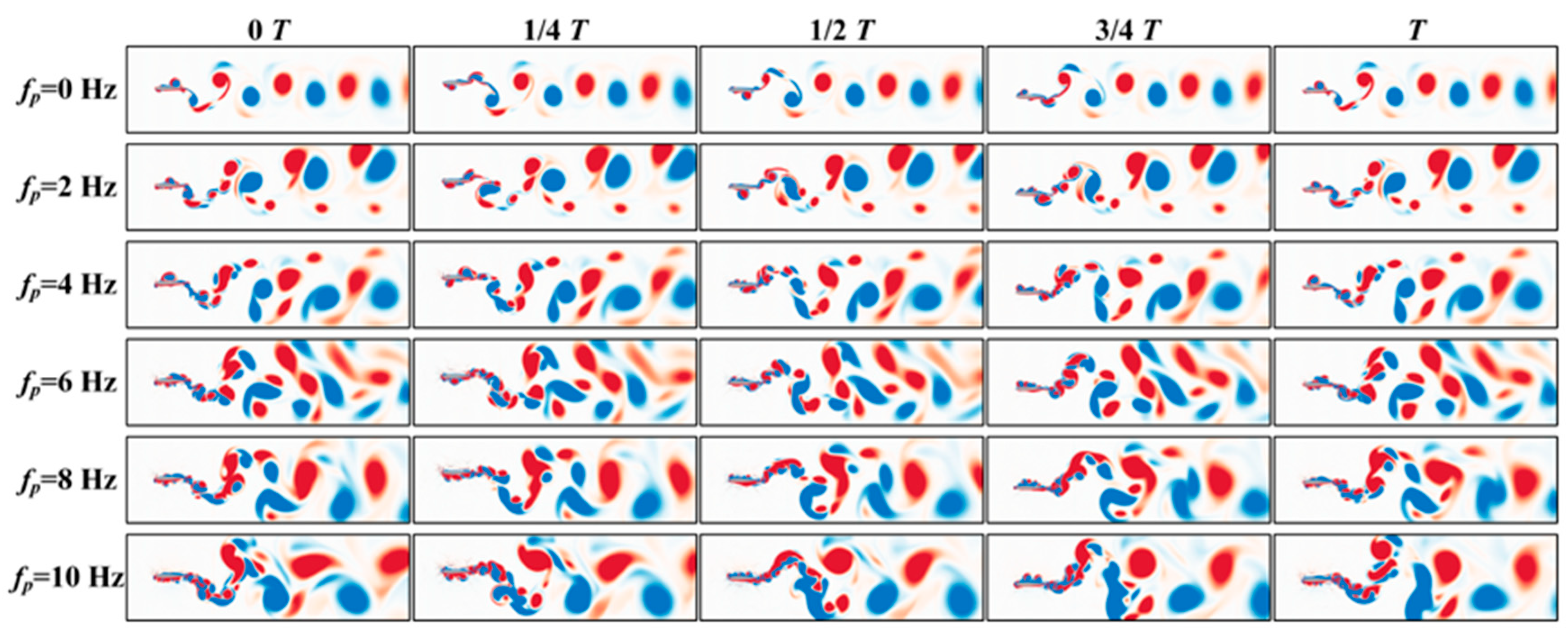
Because the flow structure is similar, this paper only shows the wake structure of the heaving foil at different perturbation frequencies at five different moments (0 T, 1/4 T, 1/2 T, 3/4 T, T) in one computational period for k= −1, 2, 5, with the initial motion direction all along the positive y-axis.
From Figure 8, it can be found that at fb = 1 Hz, the wake structure behaves as an rBvk wake at fp = 0 Hz. When fp increases to 2 Hz, the wake structure is presented as asymmetric wake and the vortex pair deflects upward. When fp increases to 4 Hz, the wake structure is not chaotic and sheds four vortices respectively in one cycle; when the perturbation frequency continues to increase to 6 Hz, the trailing edge structure starts to become chaotic. As can be seen from the Figure 4b, the thrust coefficient is increased when the perturbation frequency reaches 4 Hz. The reason for this phenomenon is that the number of wake vortex pairs increases and is accompanied by an increase in vortex strength when the perturbation frequency is 4 Hz. In particular, when the perturbation frequency is greater than 6 Hz, vortices start to fall off at the leading edge of the foil and converge into the wake, further enhancing the thrust coefficient.
The wake evolution at k = 2 is shown in Figure 9. When a perturbation of 2 Hz is added, the wake structure also deflects and appears as asymmetric wake, and the degree of deflection is greater than k ≤ 0. Unlike the sine and sawtooth wave perturbations, the wake structure remains as asymmetric wake when the perturbation frequency increases to 4 Hz and becomes chaotic when the perturbation frequency reaches 6 Hz. Because of this pattern of change in wake structure, no increase in thrust coefficient is observed at a perturbation frequency of 4 Hz as at k = −1. Instead, a significant increase in thrust coefficient is observed at fp = 6 Hz. In addition, it can be observed that when the perturbation frequency is higher than 6 Hz, the vortex density and vortex intensity are significantly increased relative to those at k = −1, which also leads to a significant increase in the heaving foil thrust coefficient.
Figure 10 shows the wake structure when k = 5, in other words, when the perturbation signal is a square wave. Unlike the two evolutionary modes mentioned previously, the wake structure becomes directly chaotic when the perturbation frequency increases to 4 Hz. This fits with the phenomenon in Figure 4a that the thrust coefficient produces a large enhancement when the perturbation frequency reaches 4 Hz when k = 5. Furthermore, by comparing the wake structure diagrams for k = −1, 2, 5, it can be observed that the vortex strength is greatest when k = 5. This also explains why the square wave perturbation brings the most significant thrust improvement for the same perturbation amplitude and perturbation frequency.
From the above analysis, it can be observed that although we add different perturbation waveforms, there is no significant effect on the wake structure of the heaving foil at perturbation frequencies below 4 Hz, which means that a higher perturbation frequency is beneficial for the perturbation signal to affect the flow structure. At the same time, this can also trigger us to think about why the effect of different waveforms of perturbation on the heaving foil wake structure is only different when the perturbation frequency is more or equal to 4 Hz. Our preliminary speculation is that this perturbation frequency value is related to the parameters, such as the base frequency we selected and the amplitude ratio between the base signal and the perturbation signal, which will also be the focus of our subsequent research.
4. Conclusions
A systematic numerical investigation of the fluid dynamics around the heaving foil, including the time-averaged thrust coefficient, time-averaged input work coefficient, propulsion efficiency, and the wake structure generated by the foil, was conducted to better understand the effects of different waveform perturbations on the heaving foil force generation and wake structure, and to provide recommendations for underwater vehicle motion parameter settings from a hydrodynamic perspective. The simulation results are concluded as follows:
- The addition of any waveform perturbation increases the axial thrust, especially when a square wave (k = 5) perturbation with a frequency of 10 Hz is applied, which directly raises the thrust to 10.49 times higher than when no perturbation is added. A response function is obtained which gives the relationship between the input perturbation parameters and the thrust coefficients.
- However, the propulsion efficiency decreases gradually with the increase of the perturbation frequency, especially when a sawtooth wave perturbation (k = −1) is applied, which brings limited thrust gain but a rapid decrease in the propulsion efficiency.
- The wake structure is roughly the same for different waveform perturbations, all of which first go through an asymmetric wake phase (at fp = 2 Hz). With increasing perturbation frequency, adding sine wave perturbation (k = 0) and sawtooth wave perturbation (k = −1, −0.8) leads to a complex wake phase (at fp = 4 Hz) and then evolves to a chaotic wake; adding square wave perturbation (k =2) keeps the asymmetric wake at fp = 4 Hz and then evolves to a chaotic wake; adding square wave perturbation (k = 5) leads to a direct evolution from an asymmetric wake to a chaotic wake.
- The simulation results have a guiding meaning for the setting of the vehicle motion parameters. The control signal of the vehicle tries to avoid the use of sawtooth wave signal. It can consider sacrificing part of the propulsion efficiency and adding a square wave signal to the drive signal to promote the vehicle gaining greater thrust. To ensure high propulsion efficiency for a long voyage, a sinusoidal signal (or a signal with k = −0.8) can be added to the drive signal. The waveform signal with k = 2 seems to be the most cost-effective choice, which provides a larger thrust without a significant decrease in propulsion efficiency.
Author Contributions
Conceptualization, P.G.; methodology, P.G.; software, P.G.; validation, P.G., Q.H., and G.P.; formal analysis, P.G.; investigation, P.G.; data curation, P.G.; writing—original draft preparation, P.G.; writing—review and editing, Q.H.; visualization, P.G.; supervision, G.P. and Q.H.; project administration, G.P. and Q.H.; funding acquisition, G.P. and Q.H. All authors have read and agreed to the published version of the manuscript.
Funding
This work was supported by the National Natural Science Foundation of China (Grant No. 51879220), the National Key Research and Development Program of China (Grant No. 2020YFB1313201), and Fundamental Research Funds for the Central Universities (Grant No. 3102019HHZY030019 and 3102020HHZY030018).
Institutional Review Board Statement
Not applicable.
Informed Consent Statement
Not applicable.
Data Availability Statement
The data that support the findings of this study are available within the article.
Conflicts of Interest
The authors declare no conflict of interest.
References
- Garrick, I.E. Propulsion of a flapping and oscillating airfoil. NACA Rep. 1937, 567, 419–427. [Google Scholar]
- Gray, J. Studies in animal locomotion: VI. The propulsive powers of the dolphin. J. Exp. Biol. 1936, 13, 192–199. [Google Scholar] [CrossRef]
- Lighthill, M.J. Hydromechanics of aquatic animal propulsion. Annu. Rev. Fluid Mech. 1969, 1, 413–446. [Google Scholar] [CrossRef]
- Wu, T.Y. Fish swimming and bird/insect flight. Annu. Rev. Fluid Mech. 2011, 43, 25–58. [Google Scholar] [CrossRef]
- Shiau, J.; Watson, J.R.; Cramp, R.L.; Gordos, M.A.; Franklin, C.E. Interactions between water depth, velocity and body size on fish swimming performance: Implications for culvert hydrodynamics. Ecol. Eng. 2020, 156, 105987. [Google Scholar] [CrossRef]
- Downie, A.T.; Illing, B.; Faria, A.M.; Rummer, J.L. Swimming performance of marine fish larvae: Review of a universal trait under ecological and environmental pressure. Rev. Fish Biol. Fish. 2020, 30, 93–108. [Google Scholar] [CrossRef]
- Russo, R.S.; Blemker, S.S.; Fish, F.E.; Bart-Smith, H. Biomechanical model of batoid (skates and rays) pectoral fins predicts the influence of skeletal structure on fin kinematics: Implications for bio-inspired design. Bioinspiration Biomim. 2015, 10, 046002. [Google Scholar] [CrossRef] [PubMed] [Green Version]
- Tytell, E.D.; Leftwich, M.C.; Hsu, C.Y.; Griffith, B.E.; Cohen, A.H.; Smits, A.J.; Hamlet, C.; Fauci, L.J. Role of body stiffness in undulatory swimming: Insights from robotic and computational models. Phys. Rev. Fluids. 2016, 1, 073202. [Google Scholar] [CrossRef]
- Mao, L.; Wang, H.; Li, Y.; Yi, H. Force model of flapping foil stabilizers based on CFD parameterization. Ocean Eng. 2019, 187, 106151. [Google Scholar] [CrossRef]
- Wu, W. Study on the self-propulsion of the rigid-flexible composite plate. Fluid Dyn. Res. 2021, 53, 045501. [Google Scholar] [CrossRef]
- Cros, A.; Castro, R.F.A. Experimental study on the resonance frequencies of a cantilevered plate in air flow. J. Sound Vib. 2016, 363, 240–246. [Google Scholar] [CrossRef]
- Eloy, C.; Souilliez, C.; Schouveiler, L. Flutter of a rectangular plate. J. Fluids Struct. 2007, 23, 904–919. [Google Scholar] [CrossRef]
- Michelin, S.; Llewellyn Smith, S.G. Resonance and propulsion performance of a heaving flexible wing. Phys. Fluids 2009, 21, 071902. [Google Scholar] [CrossRef] [Green Version]
- Root, R.G.; Courtland, H.W.; Shepherd, W.; Long, J.H. Flapping flexible fish. In Animal Locomotion, 1st ed.; Taylor, G.K., Triantafyllou, M.S., Tropea, C., Eds.; Springer: Berlin/Heidelberg, Germany, 2010; pp. 141–159. [Google Scholar]
- Root, R.G.; Liew, C.W. Computational and mathematical modeling of the effects of tailbeat frequency and flexural stiffness in swimming fish. Zoology 2014, 117, 81–85. [Google Scholar] [CrossRef]
- Grillner, S. Neural control of locomotion in lower vertebrates: From behavior to ionic mechanisms. Neural Control. Rhythm. Mov. Vertebr. 1988, 1, 1–40. [Google Scholar]
- Pearson, K.G. Common principles of motor control in vertebrates and invertebrates. Annu. Rev. Neurosci. 1993, 16, 265–297. [Google Scholar] [CrossRef]
- Pearson, K.G. Generating the walking gait: Role of sensory feedback. Prog. Brain Res. 2004, 143, 123–129. [Google Scholar] [PubMed]
- Lehn, A.M.; Thornycroft, P.J.; Lauder, G.V.; Leftwich, M.C. Effect of input perturbation on the performance and wake dynamics of aquatic propulsion in heaving flexible foils. Phys. Rev. Fluids 2017, 2, 023101. [Google Scholar] [CrossRef]
- Lu, K.; Xie, Y.H.; Zhang, D. Numerical study of large amplitude, nonsinusoidal motion and camber effects on pitching airfoil propulsion. J. Fluids Struct. 2013, 36, 184–194. [Google Scholar] [CrossRef]
- Read, D.A.; Hover, F.S.; Triantafyllou, M.S. Forces on oscillating foils for propulsion and maneuvering. J. Fluids Struct. 2003, 17, 163–183. [Google Scholar] [CrossRef]
- Heathcote, S.; Gursul, I. Jet switching phenomenon for a periodically plunging airfoil. Phys. Fluids 2007, 19, 027104. [Google Scholar] [CrossRef]
- Ashraf, M.A.; Young, J.; Lai, J.C.S. Oscillation frequency and amplitude effects on plunging airfoil propulsion and flow periodicity. AIAA J. 2012, 50, 2308–2324. [Google Scholar] [CrossRef]
- Gao, P.; Huang, Q.; Pan, G.; Zhao, J. Effects of flexibility and motion parameters on a flapping foil at zero freestream velocity. Ocean Eng. 2021, 242, 110061. [Google Scholar] [CrossRef]
Figure 1.
Schematic diagram of the flow field.

Figure 2.
Variation of the perturbation signal waveform in one period at different k.

Figure 3.
Validation for present numerical simulation: (a) grid independence verification, (b) calculation method validation and (c) validation for present numerical simulation.
Figure 3.
Validation for present numerical simulation: (a) grid independence verification, (b) calculation method validation and (c) validation for present numerical simulation.

Figure 4.
Variation of thrust coefficient: (a) a square wave vs. a sine wave and (b) a sawtooth wave vs. a sine wave.
Figure 4.
Variation of thrust coefficient: (a) a square wave vs. a sine wave and (b) a sawtooth wave vs. a sine wave.
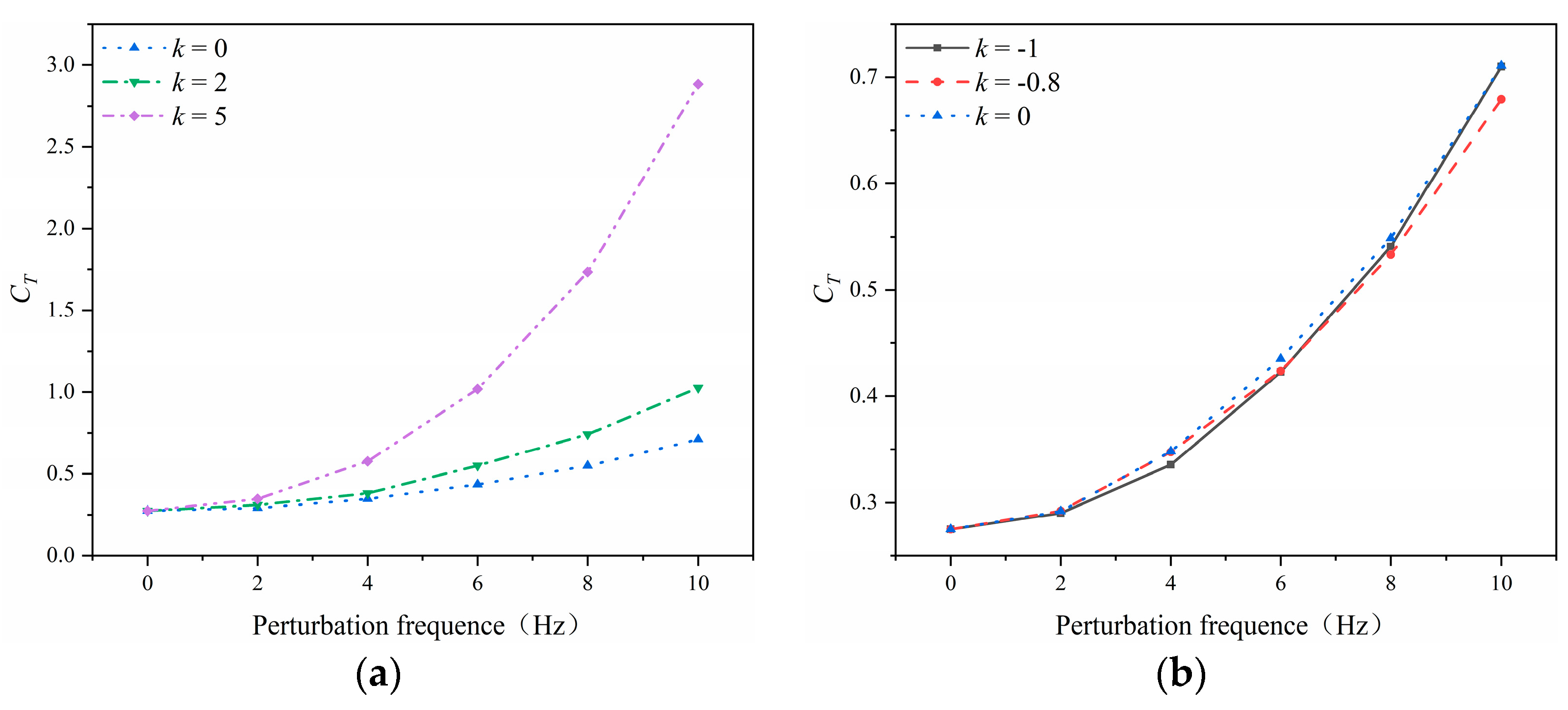
Figure 5.
Variation of propulsion efficiency.
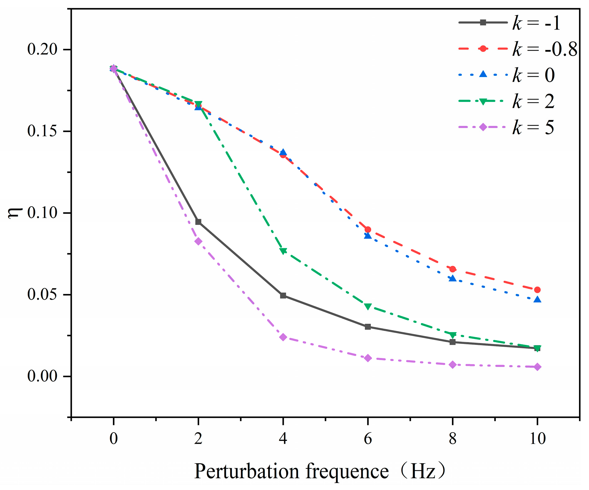
Figure 6.
Variation of input power coefficient.

Figure 7.
The numerical points in the (k, fp) plane for the heaving foil. ○: reverse Bénard–von Kármán (rBvk) wake; ●: asymmetric wake; ❊: complex wake; ◊: chaotic wake. (a) Represents the (k, fp) map and (b) presents examples of the wake structures.
Figure 7.
The numerical points in the (k, fp) plane for the heaving foil. ○: reverse Bénard–von Kármán (rBvk) wake; ●: asymmetric wake; ❊: complex wake; ◊: chaotic wake. (a) Represents the (k, fp) map and (b) presents examples of the wake structures.

Figure 8.
Instantaneous wake structure for foil at k = −1.
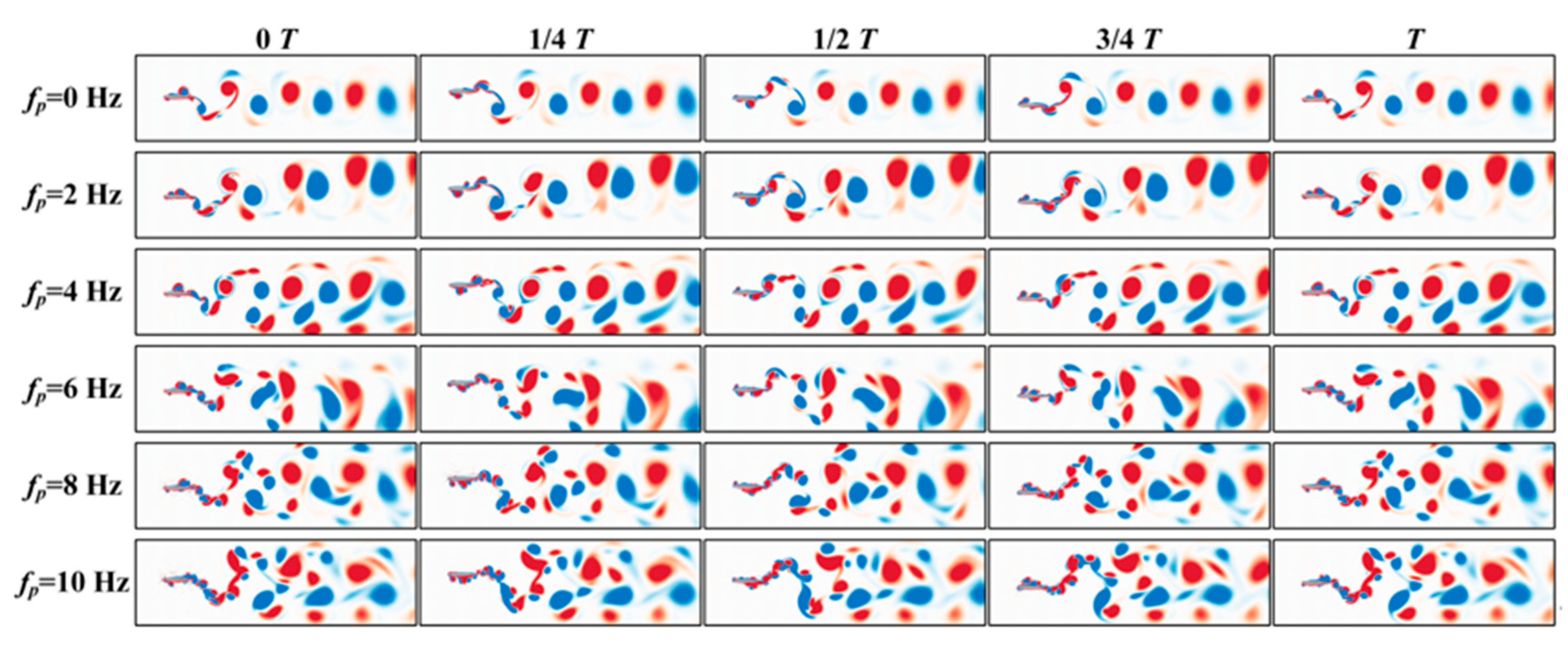
Figure 9.
Instantaneous wake structure for foil at k = 2.

Figure 10.
Instantaneous wake structure for foil at k = 5.
Publisher’s Note: MDPI stays neutral with regard to jurisdictional claims in published maps and institutional affiliations. |
© 2021 by the authors. Licensee MDPI, Basel, Switzerland. This article is an open access article distributed under the terms and conditions of the Creative Commons Attribution (CC BY) license (https://creativecommons.org/licenses/by/4.0/).
Share and Cite
MDPI and ACS Style
Gao, P.; Huang, Q.; Pan, G. Propulsion Performance and Wake Dynamics of Heaving Foils under Different Waveform Input Perturbations. J. Mar. Sci. Eng. 2021, 9, 1271. https://doi.org/10.3390/jmse9111271
AMA Style
Gao P, Huang Q, Pan G. Propulsion Performance and Wake Dynamics of Heaving Foils under Different Waveform Input Perturbations. Journal of Marine Science and Engineering. 2021; 9(11):1271. https://doi.org/10.3390/jmse9111271
Chicago/Turabian StyleGao, Pengcheng, Qiaogao Huang, and Guang Pan. 2021. "Propulsion Performance and Wake Dynamics of Heaving Foils under Different Waveform Input Perturbations" Journal of Marine Science and Engineering 9, no. 11: 1271. https://doi.org/10.3390/jmse9111271
Note that from the first issue of 2016, this journal uses article numbers instead of page numbers. See further details here.