Simulated Autonomous Driving Using Reinforcement Learning: A Comparative Study on Unity’s ML-Agents Framework

Abstract

Advancements in artificial intelligence are leading researchers to find use cases that were not as straightforward to solve in the past. The use case of simulated autonomous driving has been known as a notoriously difficult task to automate, but advancements in the field of reinforcement learning have made it possible to reach satisfactory results. In this paper, we explore the use of the Unity ML-Agents toolkit to train intelligent agents to navigate a racing track in a simulated environment using RL algorithms. The paper compares the performance of several different RL algorithms and configurations on the task of training kart agents to successfully traverse a racing track and identifies the most effective approach for training kart agents to navigate a racing track and avoid obstacles in that track. The best results, value loss of 0.0013 and a cumulative reward of 0.761, were yielded using the Proximal Policy Optimization algorithm. After successfully choosing a model and algorithm that can traverse the track with ease, different objects were added to the track and another model (which used behavioral cloning as a pre-training option) was trained to avoid such obstacles. The aforementioned model resulted in a value loss of 0.001 and a cumulative reward of 0.068, proving that behavioral cloning can help achieve satisfactory results where the in game agents are able to avoid obstacles more efficiently and complete the track with human-like performance, allowing for a deployment of intelligent agents in racing simulators.

1. Introduction

Reinforcement learning (RL) is a powerful approach for training intelligent agents to perform a wide range of tasks, from playing games to navigating complex environments [1]. The possible applications include the following: robotics, where RL can be used to train robots to perform tasks such as grasping objects or navigating through a physical environment [2] with strong potential to drive adapting industrial environments, a potential technological driver to emerge under the revolution of Industry 4.0 [3]; game playing, where RL has been used to train agents to play games [4] such as chess, Go and poker at a superhuman level; Autonomous vehicles, where RL can be used to train self-driving cars to make decisions [5] such as when to change lanes or when to stop at a traffic light; healthcare, where RL can be used to optimize treatment plans for patients and to design personalized medicine [6,7]; industrial control, where RL can be used to optimize control of industrial systems [8,9] such as power grids, water treatment plants and factories; energy, where RL can be used to optimize energy consumption [10], renewable energy systems and storage; recommendation systems, where RL can be used to optimize personalized recommendations for users [11], such as products or movies to watch; cybersecurity, where RL can be used to train agents to detect and respond to cyber attacks [12].

One particularly promising application of RL is in the development of autonomous racing agents [13,14], which can navigate a racing track and make decisions about how to navigate obstacles and other competitors in real time. In most cases, particularly for testing, simulation environments are used [15,16]. One key advantage of using simulation environments for the training of RL agents is the ability to easily generate large amounts of data for training and testing. This is particularly important for tasks such as autonomous driving [17] and autonomous path planning [18,19] and tracking control [20,21], where real-world data can be difficult and expensive to collect. Simulation environments also allow for greater control over the training environment, enabling researchers to easily vary factors such as the layout of the track or the weather conditions [22].

The development of autonomous racing agents is important for mobile robotics because it presents a challenging problem that requires the integration of many different skills, including perception, control, path planning [23] and decision-making. Autonomous racing involves navigating through a dynamic, unstructured environment at high speeds while avoiding obstacles, moving over irregular terrain [24,25] and competing against other agents. Solving this problem requires the development of advanced algorithms for perception, control and decision-making, as well as the ability to process large amounts of data in real time. Additionally, the use of simulation environments allows for the safe and efficient testing of these agents in crowded environments [19] or partially unknown environments [26], which is important when working with mobile robots. The development of autonomous racing agents can also lead to the development of more capable mobile robots that can be used in a variety of different applications, such as search and rescue, delivery and other tasks. The development of autonomous racing agents can also lead to important breakthroughs in the field of robotics, as the challenges that need to be overcome for autonomous racing are similar to those that need to be overcome for other mobile robotic applications. In addition, autonomous racing can serve as a test bed for various technologies, such as sensors, cameras, lidars and other technologies that can be used in mobile robotics [27,28]. These technologies are then further improved to meet the demands of autonomous racing and then can be used in other mobile robotic applications.

In this paper, we investigate the the Unity ML-Agents toolkit [29], a widely used platform for training intelligent agents using RL algorithms, to train kart agents to navigate a racing track. The Unity engine [30] provides a rich and realistic simulation environment that allows for the development and testing of intelligent agents in a wide range of scenarios. By training kart agents to navigate a racing track using RL algorithms, we aim to identify the most effective approach for training autonomous racing agents. The novelty of this paper is that it explores the use of the Unity ML-Agents toolkit to train intelligent agents to navigate a racing track in a simulated environment using RL algorithms.

The paper contributes to the field by comparing the performance of several RL algorithms, including Multi-Agent Proximal Policy Optimization (MA-PPO) and POCA (Parallel Online Continuous Arcing), in training intelligent agents to navigate a racing track in a simulated environment. Additionally, the paper proposes the use of behavioral cloning as a pre-training condition with the default PPO algorithm to assist the model in learning the required behavior and to improve the performance of intelligent agents for solving the racing task. The paper also provides insight into the capabilities and limitations of different RL algorithms and can inform the development of more effective and efficient approaches for training intelligent agents in simulated environments. Our results provide insight into the relative strengths and weaknesses of different RL approaches and contribute to the growing body of literature on the use of RL algorithms for training intelligent agents in simulated environments [31,32].

2. State of the Art Review

There have been numerous advances in reinforcement learning algorithms for training intelligent agents to perform tasks in simulated environments [33], such as using the Unity engine [34]. One example is the use of deep RL, which combines the use of deep neural networks with RL algorithms to enable the learning of complex tasks from high-dimensional sensory input [35]. This approach has been applied to a range of tasks in simulated environments, including the training of autonomous vehicles to navigate roads and traffic [36].

Another notable development in RL for simulation environments is the use of multi-agent RL algorithms, which enable the training of multiple agents to interact and learn from one another in a shared environment [37]. This has the potential to enable the development of more complex and realistic simulations, as well as to facilitate the training of agents to perform collaborative tasks. In addition, there has been a growing interest in the use of RL algorithms for training autonomous racing agents to navigate tracks in simulation environments [38]. These approaches often involve the use of actor–critic algorithms, which learn to predict the value of different actions in a given state and use this information to guide the selection of actions [39]. In another paper, the authors [40] extend the Generative Adversarial Imitation Learning (GAIL) approach of Reinforcement learning (which uses human-provided inputs) to solve shortcomings when training several agents. They propose parameters sharing GAIL which proves superior to GAIL in interacting stably in a multi-agent environment. In the paper [41], the author presents an RL-based approach where multiple agents cooperate and coordinate their actions in a simulated traffic environment. The author uses a deep RL to train said agents to improve and optimize the actions made based on actions of other agents in the environment. The author proposes a reward function that takes into consideration not only the performance of each agent, but additionally the total performance of the whole system. The author also introduces a mechanism for the agents to communicate and share information of the actions performed in certain conditions and what results that leads to. Temporal information and historical data can also be used to train agents to traverse roads and tracks. In the paper [42], the authors used Convolutional Neural Networks (CNN) to extract features from the road, after which an LSTM (long short term memory) network is used to choose an action based on historical data of different actions taken based on different features extracted. The approach was tested on the open racing car simulator and has been able to mimic human decisions with a relatively high degree of accuracy.

Some approaches use both real-world and simulated environments to train and improve models in autonomous driving environments [43]. Deep and traditional RL-based models can be trained on simulated agents, after which the models are fine tuned in real-world environments where the model is fine tuned to perform more in line with what is expected [44]. The authors of [45] suggest a comprehensive learning approach for self-driving systems which utilizes neural networks to approximate suitable motor commands from sensory input. The authors tackle the issue of returning a car to its designated lane when it deviates off course by gathering recovery data based on the distance from a preferred track while conducting a road test using a simulator. The proposed method consists of three phases: firstly, data are gathered by means of a path-following module during a hundred laps of driving; secondly, a neural driving module is trained using these data to generate driving behavior, such as adjusting the accelerator, brake and steering based on a particular threshold; finally, the neural driving module is re-trained using data collected from the path-following module during another hundred laps of driving. The efficacy of the proposed approach is assessed by comparing the average distance from the nearest waypoint link and the average distance traveled per lap across datasets with no recovery, random recovery and the proposed method with recovery. The findings demonstrate that the model based on the proposed method performed well and demonstrated a greater focus on the road as opposed to unrelated objects, across both trained and untrained courses and various weather conditions.

We compare the discussed studies based on their application domain, reinforcement learning algorithm used and performance metrics in

Table 1. Comparison of studies based on application domain, reinforcement learning algorithms and performance metrics.

Study	Application Domain	RL Algorithm	Performance Metrics
[33]	virtual vehicle simulation	PPO and BC	torque, steering, acceleration, rapidity, revolutions per minute (RPM) and gear number
[35]	game playing	deep Q-learning with experience replay	win rate
[36]	autonomous driving	-	autonomy
[37]	robotics	MADDPG	communication success
[38]	autonomous driving	soft actor–critic and rainbow DQN	angle, track position, speed, wheel speeds, RPM
[39]	pole balancing	associative search element (ASE) and adaptive critic element (ACE)	score
[40]	autonomous driving	Parameter Sharing Generative Adversarial Imitation Learning (GAIL)	RMSE
[41]	autonomous driving	DQN	successful intersection crossings
[42]	autonomous driving	DQN	driving decisions
[43]	robotics	DQN	distance run
[44]	robotics	A3C (Asynchronous Advantage Actor–Critic), PPO	OpenAI Gym benchmark metrics
[45]	autonomous driving	-	distance travelled

.

The state of the art in RL algorithms for simulation environments continues to evolve, with ongoing research focused on developing more efficient and effective approaches for training intelligent agents to perform a wide range of tasks. RL algorithms have been increasingly used to train agents to perform tasks in simulated environments, such as the Unity engine. Deep RL, which combines deep neural networks with RL algorithms, has been used to learn complex tasks from high-dimensional sensory input, such as training autonomous vehicles to navigate roads and traffic. Multi-agent RL algorithms have also been developed, allowing the training of multiple agents to interact and learn from one another in a shared environment. These have potential for the development of more complex and realistic simulations, as well as the training of agents to perform collaborative tasks. RL approaches have also been used to train autonomous racing agents to navigate tracks in simulation environments using actor–critic algorithms and to train multiple agents to cooperate and coordinate actions in a simulated traffic environment. CNNs and LSTMs have been used to extract features from the road and historical data to choose actions for autonomous driving. Some approaches use both real-world and simulated environments to train and fine tune models in autonomous driving environments.

3. Materials and Methods

3.1. Reinforcement Learning for Autonomous Cart Racing

Reinforcement learning (RL) is a learning framework where an agent learns to make decisions by interacting with an environment. The agent’s goal is to maximize the expected cumulative reward over time. Autonomous cart racing is a task where multiple agents, represented by autonomous carts, navigate through a track while competing against each other to reach the finish line as fast as possible. A mathematical definition of RL for this task can be defined as follows:

Let there be a set of agents $A=a_1,a_2,\dots ,a_n$, where n is the total number of agents. Each agent $a_i$ is an autonomous cart that interacts with the track environment in a sequence of discrete time steps $t=1,2,\dots ,T$. At each time step t, each agent $a_i$ takes an action $a_{i,t}$ from a set of actions $A_i$, which include acceleration, braking and steering and the environment transitions to a new state $s_{t+1}$ and provides each agent with a scalar reward $r_{i,t}$. The agent’s goal is to learn a policy ${\pi }_i\left(a_{i,t}\right|s_t)$, which is a probability distribution over actions given the current state, that maximizes the expected cumulative reward over time, also known as the return, defined as:

$$J\left({\pi }_i\right)=\mathbb{E}{\pi }_i\left[\sum {t=0}^{T-1}{\gamma }^t{r}_{i,t}\right]$$

(1)

where $\gamma \in [0,1]$ is a discount factor that determines the importance of future rewards and $r_{i,t}$ is the reward associated with reaching the finish line as fast as possible, avoiding collisions and penalties. This can also be defined by considering the state value function $V_{{\pi }_i}\left(s_t\right)$ which represents the expected time to reach the finish line starting from state $s_t$ and following policy ${\pi }_i$:

$$V_{{\pi }_i}\left(s_t\right)=\mathbb{E}{\pi }_i\left[\sum {k=0}^{T-t-1}{\gamma }^k{r}_{i,t+k}\right|s_t]$$

(2)

and the action-value function $Q_{{\pi }_i}(s_t,a_{i,t})$ which represents the expected time to reach the finish line starting from state $s_t$, taking action $a_{i,t}$ and following policy ${\pi }_i$:

$$Q_{{\pi }_i}(s_t,a_{i,t})=\mathbb{E}{\pi }_i\left[\sum {k=0}^{T-t-1}{\gamma }^k{r}_{i,t+k}\right|s_t,a_{i,t}]$$

(3)

The objective of RL for multiple agents in autonomous cart racing is for each agent $a_i$ to learn a policy ${\pi }_i$ that maximizes its own expected time to reach the finish line as fast as possible while avoiding collisions and penalties.

3.2. Test Environment

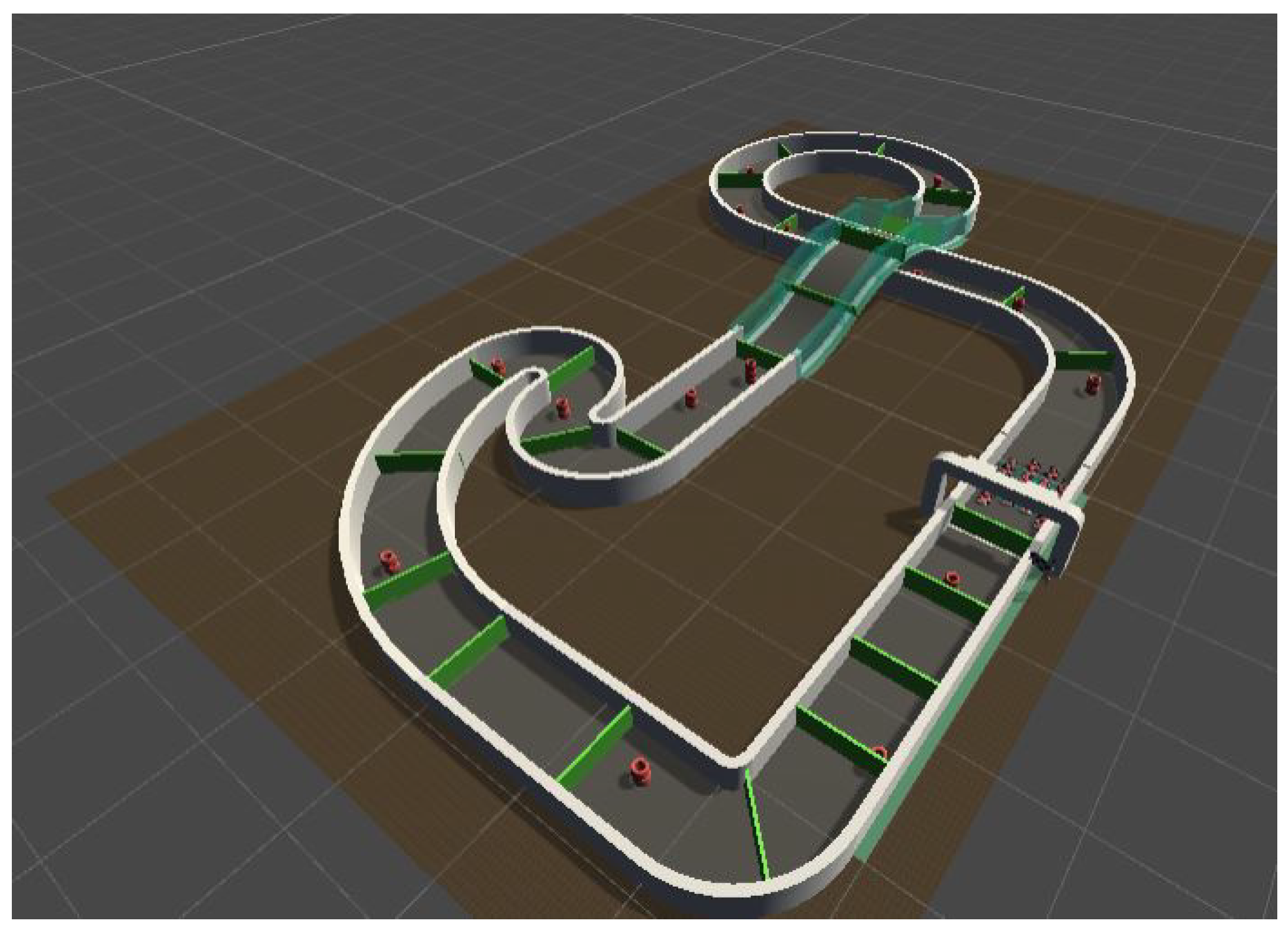
The simulation/test environment was chosen to be the Unity game engine. The experiments conducted for this project used a publicly available environment (repository name https://github.com/jaredbest/unity-ai-racing-karts-ml-agents accessed on 8 April 2023). This environment includes a racing track as well as the karts/agents. There are 24 agents in total. Multiple agents are used to speed up training. Agents are independent of each other, meaning their training occurs independently. An illustration of the environment can be seen below in Figure 1.

The environment also includes kart models that are able to traverse the track. There are 24 such karts and they are used as the agents in our experiments. There are three ways by which the agents can be controlled, one is through the usage of ML-agents, by which the ML-agent’s so-called “brain” is used to control the agents. This is the default so-called “behavior type”. The second option is the “inference only” behavior type, with which the agents use an already trained network to control the agents. The final behavior type is called “heuristic only”; with it, a user controls the agent using pre-specified keys. All three types are used during our experimentation. The 24 mentioned karts/agents can be seen in Figure 2.

The second part of the experiments included adding obstacles on the track to see if it is possible to train agents that can both traverse the track as well as avoid all obstacles. The obstacles used are simple round roadblocks. They are placed randomly along the track. Their positions will change for some of the experiments to showcase the robustness of trained models. Some of the obstacles can be seen in Figure 3.

3.3. Algorithms

In this paper two main algorithms are used, with some modifications of each to train our agents. The two algorithms are the well-known Proximal Policy Optimization (PPO) [46] and POCA [47] algorithms. Those algorithms are used as they are available in the ML-agents framework used. Both of the algorithms support multi-agent training. Training multiple independent agent speeds up training and makes good use of distributed computing.

3.3.1. MA-PPO Algorithm

The MA-PPO (Multi-Agent Proximal Policy Optimization) algorithm is a variant of the PPO (Proximal Policy Optimization) algorithm that is specifically designed for training multiple agents in a shared environment. PPO is a reinforcement learning algorithm that uses a combination of value and policy gradients to optimize the performance of an agent in an environment. It is known for being stable and relatively easy to implement compared to other reinforcement learning algorithms. The MA-PPO algorithm extends the standard PPO algorithm to work with multiple agents, allowing them to learn and interact with each other within a shared environment. This can be useful for training agents to coordinate their actions, such as in multi-agent games or simulations, including for the task of autonomous cart racing. The MA-PPO algorithm can be defined as follows:

Let there be a set of agents $A=a_1,a_2,\dots ,a_n$, where n is the total number of agents. Each agent $a_i$ has a policy ${\pi }_i\left(a_{i,t}\right|s_t;{\theta }_i)$ that is parameterized via ${\theta }_i$, where ${\pi }_i$ is a probability distribution over actions given the current state. The objective of the MA-PPO algorithm is to find the policy parameter ${\theta }_i$ that maximizes the expected cumulative reward over time, also known as the return, defined as:

$$J\left({\pi }_i\right)=\mathbb{E}{\pi }_i\left[\sum {t=0}^{T-1}{\gamma }^t{r}_{i,t}\right]$$

(4)

where $\gamma \in [0,1]$ is a discount factor that determines the importance of future rewards.

The MA-PPO algorithm updates the policy parameters ${\theta }_i$ by maximizing a surrogate objective function $L^{MA-PPO}\left({\theta }_i\right)$ defined as:

$$L^{MA-PPO}\left({\theta }_i\right)={\mathbb{E}}_{\tau \sim {\pi }_i}\left[min\left(r_t\left({\theta }_i\right)\frac{{\pi }_i\left(a_t\right|s_t;{\theta }_i)}{{\pi }_i\left(a_t\right|s_t;{\theta }_i^{\mathrm{old}})},clip(r_t\left({\theta }_i\right),1-ϵ,1+ϵ)\right)\right]$$

(5)

where $\tau$ is the trajectory of the agent, $r_t\left({\theta }_i\right)$ is the likelihood ratio between the new and old policy, ${\pi }_i\left(a_t\right|s_t;{\theta }_i)$ and ${\pi }_i\left(a_t\right|s_t;{\theta }_i^{\mathrm{old}})$, respectively, and $ϵ$ is a hyperparameter that controls the step size.

The MA-PPO algorithm repeatedly updates the policy parameters ${\theta }_i$ by performing gradient ascent on the surrogate objective function $L^{MA-PPO}\left({\theta }_i\right)$ using mini-batch of trajectories sampled from the current policy. In summary, MA-PPO is a variant of PPO that can be used to train multiple agents simultaneously for the task of autonomous cart racing by updating the policy parameters ${\theta }_i$ with the goal of maximizing the expected cumulative reward over time. The MA-PPO algorithm has been shown to be effective in a variety of environments, including multi-agent games and cooperative tasks [48]. A simplified diagram of how the PPO algorithm works can be seen in Figure 4.

The pseudocode of the PPO can be seen in Algorithm 1:

Algorithm 1 MA-PPO algorithm

1: Initialize a policy network $\pi$ and a value network V   2: Initialize a set of parameters $\theta$ for the policy and value networks   3: Initialize a set of old parameters ${\theta }_{old}$ for the policy and value networks   4: Initialize a set of trajectories $\tau =\left\{\right\}$   5: for each iteration do   6:       Reset the environment and get initial state $s_0$   7:       for each time step do   8:           Sample an action $a_t$ from the current policy ${\pi }_{\theta }$   9:           Execute action $a_t$ and observe reward $r_t$ and new state $s_{t+1}$ 10:           Store the transition tuple $(s_t,a_t,r_t,s_{t+1})$ in $\tau$ 11:           Update the value network: $V_{\theta }\left(s_t\right)\leftarrow V_{\theta }\left(s_t\right)+\alpha (r_t+\gamma V_{\theta }\left(s_{t+1}\right)-V_{\theta }\left(s_t\right))$ 12:       end for 13:       Calculate the advantages using the GAE ($\tau \leftarrow$ compute_advantages($\tau ,\gamma ,\lambda$)) 14:       Normalize the advantages 15:       Update the old policy parameters: ${\theta }_{old}\leftarrow \theta$ 16:       Optimize the policy using the PPO objective: $\theta \leftarrow$ optimize_policy($\tau ,\theta ,{\theta }_{old}$) 17: end for

3.3.2. POCA Algorithm

POCA (Parallel Online Continuous Arcing) [49] is a boosting algorithm that differs from traditional arcing algorithms such as Adaboost. While traditional arcing algorithms construct an ensemble by adding and training weak learners sequentially on a round-by-round basis, POCA performs training over an entire ensemble continuously and in parallel. This allows POCA to adapt rapidly to non-stationary environments, as members of the ensemble are not frozen after an initial learning period. Additionally, POCA does not require the explicit storage of exemplar statistics, making it capable of online learning. As a result, POCA is a boosting algorithm that trains an ensemble of weak learners in parallel and continuously, enabling fast adaptation to non-stationary environments and online learning capabilities. In Figure 5, a simplified view of the way POCA algorithm works can be seen. The pseudocode can be seen in Algorithm 2.

Algorithm 2 POCA

1: Initialize a set of policies ${\pi }_1,{\pi }_2,\dots ,{\pi }_N$ for each agent   2: Initialize a set of value functions $V_1,V_2,\dots ,V_N$ for each agent   3: Initialize a set of parameters ${\theta }_1,{\theta }_2,\dots ,{\theta }_N$ for the policy and value functions of each agent   4: Initialize a set of old parameters ${\theta }_{old,1},{\theta }_{old,2},\dots ,{\theta }_{old,N}$ for the policy and value functions of each agent   5: Initialize a set of trajectories $\tau =\left\{\right\}$   6: for each iteration do   7:       Reset the environment and get initial state $s_0$   8:       for each time step do   9:          Sample actions $a_{1,t},a_{2,t},\dots ,a_{N,t}$ from the current policies ${\pi }_{1,{\theta }_1},{\pi }_{2,{\theta }_2},\dots ,{\pi }_{N,{\theta }_N}$ 10:          Execute actions $a_{1,t},a_{2,t},\dots ,a_{N,t}$ and observe rewards $r_{1,t},r_{2,t},\dots ,r_{N,t}$ and new state $s_{t+1}$ 11:          Store the transition tuples $(s_t,a_{1,t},a_{2,t},\dots ,a_{N,t},r_{1,t},r_{2,t},\dots ,r_{N,t},s_{t+1})$ in $\tau$ 12:          Update the value functions: $V_{i,{\theta }_i}\left(s_t\right)\leftarrow V_{i,{\theta }_i}\left(s_t\right)+\alpha (r_{i,t}+\gamma V_{i,{\theta }_i}\left(s_{t+1}\right)-V_{i,{\theta }_i}\left(s_t\right))$ for all agents i 13:       end for 14:       Calculate the advantages using the GAE ($\tau \leftarrow$ compute_advantages($\tau ,\gamma ,\lambda$)) 15:       Normalize the advantages 16:       Update the old policy parameters: ${\theta }_{old,i}\leftarrow {\theta }_i$ for all agents i 17:       Optimize the policies using the MPOCA objective: ${\theta }_i\leftarrow$ optimize_policy($\tau ,{\theta }_i,{\theta }_{old,i}$) for all agents i 18: end for

3.4. Reward Structure of the Implementation

The reward structure of the environment was not edited except for the addition of punishment/negative reward in the case of the added obstacles. The list below explains, without going into detail, how the episodes are portrayed and when rewards or punishments are added.

• Agents begin at the starting position where the ML-agents’ ‘brain’ starts listening to input and provides actions for agents to perform.
• Whenever an agent passes through a checkpoint, a reward is added to the agent’s total that equals the $0.5/n$, n here being the total number of checkpoints.
• If the time to reach the next checkpoint exceeds 30 s, the episode ends, the agent receives a punishment of −1 and the agent respawns at the start of the track.
• Whenever the agent reaches the final checkpoint, a reward of 0.5 is given, the episode ends and the agent respawns at the starting position.
• To incentivize speed, agents are given a small −0.001 reward (punishment).
• In the case of the added obstacles version of the environment, a negative reward of −0.1 is given every time a collision occurs between the agent and any of the obstacles.

This can also be summarized in the pseudocode available in Algorithm 3.

3.5. Agents Sequence Diagram

The sequence diagram in Figure 6 shows how the ML-agent clients use the ML-Agents Server to understand the environment. If the agent successfully navigates past checkpoints and obstacles with $Action\left(A_t\right)$, it receives a $Reward\left(R_t\right)$ from the ML-Agents server. However, if the agent is not efficient, it receives a $Punishment\left(P_t\right)$ and returns to the server with a $State\left(S_n\right)$ to receive the next $Action\left(A_{t+1}\right)$ and $Reward\left(R_{t+1}\right)$. This process repeats multiple times, with the agent receiving different $Action\left(A_{t+n}\right)$, $Reward\left(R_{t+n}\right)$, $Punishment\left(R_{t+n}\right)$ and $State\left(S_{t+n}\right)$.

Algorithm 3 Reward structure

1: Input: kart agents, track, obstacles (optional)   2: Output: trained kart agents   3: Initialize: agents at starting position, total reward = 0, total number of checkpoints = n   4: repeat   5:       Begin episode:   6:       while agent has not reached final checkpoint do   7:          agent performs actions based on input and brain’s output   8:          if agent passes through checkpoint then   9:              total reward += 0.5/n 10:          end if 11:          if time to reach next checkpoint > 30 s then 12:              end episode 13:              agent receives punishment of −1 14:              agents respawn at start of track 15:          end if 16:          if agent collides with obstacles (added version only) then 17:              total reward += −0.1 18:          end if 19:          agent receives punishment of −0.001 for every time step 20:       end while 21:       End episode: 22:       agent receives reward of 0.5 23:       agents respawn at start of track 24: until agents are sufficiently trained

4. Experimental Evaluation and Results

4.1. Settings

The evaluation of the different experiments carried out is carried out by comparing the mean reward for all karts in the final step. The results of the rewards of the experiments carried out with and without obstacles should not be directly compared, as having obstacles slows down and thus adds a significant negative reward to agents. Thus, we first compare different algorithms using the default environment where obstacles were not added and select the algorithm/model with the highest mean reward. For experiments that include obstacles, the best algorithm from the previous steps is used to train the agents. Experiments carried out in the environment with added obstacles on the track are evaluated separately.

The experiments shall be divided into two main sections and further subsections. These are listed below.

• Environment without obstacles.

  -

  Default models.

  *

  Default PPO algorithm configurations.

  *

  Default POCA algorithm configurations.

  *

  ML-agents default, which also uses the PPO algorithm.

  *

  Adding RNN to the best model from the default models.

• Environment with obstacles.

  -

  Default PPO algorithm.

  -

  Adding behavioral cloning as a pre-training condition with the default PPO algorithm

Before going into the results, we must first look at the tools used to perform those experiments. In

Table 2. Hardware and software used.

Hardware	GPU	Pipelines	Video Memory	Memory Type
	Nvidia 1650 ti	1024	4 GB	GDDR6
Software	Unity Editor Version	ML-Agents Package Version	Pytorch Version	CUDA Version	Python Version
	2020.3.39f1	0.29.0	1.8.0 + cu111	11.4	3.8.0

, both the hardware and software used can be seen.

4.2. Results

4.2.1. Environment without Obstacles

First we train and compare different models in the default environment without obstacles. This will be divided into two, the default models and the best model chosen with added RNA as (1) default models and (2) default model of the ML-agents.

First, the default ML-agents model was experimented with. The results were not satisfactory as the agents were unable to navigate the track easily and did not produce decent rewards or loss of value. The model yielded a mean cumulative reward of −1.582 and a value loss of 0.006. The plots of the model can be seen in Figure 7. This model uses the configurations seen in

Table 3. ML-agent’s default model configurations.

Parameter	Value
batch_size	1024
buffer_size	10,240
learning_rate	0.0003
beta	0.005
epsilon	0.2
lambda	0.95
num_epoch	30
learning_rate_schedule	linear

.

4.2.2. Default PPO Model (Also Environment’s Default)

The default PPO model was experimented with and yielded the best results with a mean cumulative reward and value loss of 0.761 and 0.0013, respectively. The plots of the model can be seen in Figure 8. This model uses the configurations seen in

Table 4. Configurations of the default PPO model.

Parameter	Value
batch_size	120
buffer_size	12,000
learning_rate	0.0003
beta	0.001
epsilon	0.2
lambda	0.95
num_epoch	30
learning_rate_schedule	linear

.

4.2.3. Default POCA Model

The default POCA model achieved decent results with a cumulative reward and value loss of −0.372 and 0.002, respectively. The plots of the model can be seen in Figure 9. This model uses the configurations seen in Table 4.

Adding memory or RNN blocks to the model was attempted with the results shown below. The cumulative reward degraded with the number of steps and did not reach satisfactory results after the set number of steps with a final reward of −2.411 and a loss of 0.082. The plots of the model can be seen in Figure 10. This model uses the configurations seen in

Table 5. PPO model with added memory.

Parameter	Value
batch_size	1024
buffer_size	10,240
learning_rate	0.0003
beta	0.005
epsilon	0.2
lambda	0.95
num_epoch	30
learning_rate_schedule	linear
memory_size	128
sequence_length	64

.

The next set of experiments will include an environment where obstacles were placed in random positions, where agents would be required to traverse the track and avoid any obstacles in their way.

4.2.4. Default PPO Model

The default PPO was retrained using an environment for which obstacles were added.The results were not satisfactory, with a final mean reward of −2.574 and a loss value of 0.018. The plots of the model can be seen in Figure 11. The configurations used can be found in Table 4.

The default PPO was retrained using an environment in which obstacles were added. Behavioral cloning was used here as a pre-training condition with a strength hyperparameter set to 0.1. The results were not satisfactory with a final mean reward of −2.547 and a loss value of 0.0042. The plots of the model can be seen in Figure 12. The configurations used can be found in Table 4.

After adding behavioral cloning as a pre-training condition with a strength hyper-parameter set to 1.0, agents were able to learn the desired behavior. The results were not satisfactory, with a final mean reward of 0.0681 and 0.0011. Plots of the model can be seen in Figure 13. The configurations used can be found in Table 4.

4.2.5. Comparing the Final Model on Different Obstacle Positions

As a robustness test, the final model trained on the obstacles that includes the obstacles (17 obstacles in total) was tested on three different random configurations that are listed below:

• First configuration: the figure shows the configuration that the model was trained with Figure 14a.
• Second configuration: a configuration in which obstacles were placed in different random positions, as can be seen in Figure 14b.
• Third configuration: another configuration in which obstacles were placed again in different random positions and this can be seen in Figure 14c.

To compare the model with the positions of the aforementioned obstacles, we run the model in inference mode for one minute per configuration. The metric used here is simply the number of times the agent collides with an obstacle. It is important to note here that the tests that follow were carried out on a single agent (all other agents were disabled). This is done for better interpretability and for demonstration purposes. The results are presented in Figure 15.

4.2.6. Comparing Model Sizes

To compare the size of the models, we use the actual memory size of each model in kilobytes. These do represent the sizes of the models directly as the file format used to store the models is not compressed and is stored as is. The comparison of the different model sizes can be seen in Figure 16. Every model that uses the default PPO hyperparameters has the same size (hence why we only have four bars).

5. Discussion and Future Research

5.1. Evaluation of Findings

The results of our experiments confirm the usefulness of behavioral cloning for improving the performance of intelligent agents for racing tasks. Behavioral cloning is a technique where an agent is trained to mimic the behavior of an expert. In the context of this paper, it involves training an agent using a dataset of expert demonstrations where a human-controlled kart navigates the racing track and avoids obstacles. Adding behavioral cloning as a pre-training condition with the default PPO algorithm can improve the performance of intelligent agents for solving the racing task in several ways.

• First, pre-training with behavioral cloning can help to initialize the agent’s policy network with a set of good initial weights. This can help to improve the convergence speed of the RL algorithm during training, allowing the agent to learn faster and achieve better performance.
• Secondly, behavioral cloning can help to improve the agent’s ability to generalize to new situations such as different obstacle configurations. By training the agent on a dataset of expert demonstrations that includes a variety of different scenarios and obstacle configurations (see Figure 15), the agent can learn to recognize and respond appropriately to different situations it may encounter during the racing task. This can help to improve the agent’s overall performance and reduce the likelihood of it getting stuck in local optima during training.
• Finally, adding behavioral cloning as a pre-training condition with the default PPO algorithm can improve the stability and robustness of the agent’s policy network. By training the agent to mimic the behavior of an expert, the agent can learn to avoid certain mistakes or suboptimal behaviors that may arise during the RL training process. This can help to improve the overall quality of the agent’s policy network and make it more resistant to noise and other sources of variability in the environment.

In summary, adding behavioral cloning as a pre-training condition with the default PPO algorithm can improve the performance of intelligent agents for solving the cart racing task by improving the initialization of the policy network, improving the agent’s ability to generalize to new obstacle configurations and improving the stability and robustness of the model.

5.2. Network Simplification Using Pruning Techniques

Network pruning techniques can be used to simplify deep networks used for training ML-agents using RL, which can help to reduce the number of parameters and memory usage [50,51,52]. Deep neural networks typically consist of millions of trainable parameters, which can make them computationally expensive and difficult to train. Network pruning techniques involve removing unnecessary connections or neurons from a network, which can reduce the number of parameters and improve the efficiency of the network. There are several different network pruning techniques that can be used, including weight pruning, neuron pruning and filter pruning. Weight pruning involves removing small-weight connections from the network, while neuron pruning involves removing entire neurons that are not contributing significantly to the network’s output. Filter pruning involves removing entire filters from convolutional layers that are not contributing significantly to the network’s output. By using network pruning techniques, it is possible to simplify deep networks used for training ML-agents using RL, which can reduce the number of parameters and memory usage. This can make the networks more efficient and easier to train, which can ultimately lead to better performance. Additionally, network pruning can help to reduce the risk of overfitting, as it can prevent the network from memorizing noise in the training data. Overall, network pruning techniques can be a useful tool for simplifying deep networks used for training ML-agents using RL. By reducing the number of parameters and memory usage, network pruning can make the networks more efficient and easier to train, which can ultimately lead to better performance.

5.3. Possible Applications

The use of the Unity ML-Agents toolkit to train intelligent agents to navigate a racing track in a simulated environment using RL algorithms has several potential real-world applications. One possible application is in the development of autonomous vehicles, where RL algorithms can be used to train agents to navigate complex environments and avoid obstacles. The use of a simulated environment allows for safe and efficient testing of autonomous vehicle systems before they are deployed on real roads. Another potential application is in the development of robotics, where RL algorithms can be used to train robots to perform complex tasks in a variety of environments. For example, robots could be trained to navigate through cluttered environments, such as warehouses or factories, to perform tasks such as picking and packing items. The use of RL algorithms to train intelligent agents in simulated environments can also have applications in the field of gaming. Game developers can use these algorithms to create more intelligent and realistic non-player characters (NPCs) [53,54] that can interact with players in more complex ways. Overall, the use of the Unity ML-Agents toolkit to train intelligent agents using RL algorithms has the potential to revolutionize several industries, including autonomous vehicles, robotics and gaming.

5.4. Future Research

There are many areas where this research could be expanded on. Our research has been very specific to, as is clear to, one environment and to one framework (ML-agents) which has a limited number of algorithms to choose from. To summarize areas of expansion for future research, we list them below and go into some detail concerning what each would mean.

• Expansion of the algorithms used and hyperparameters experimented with. As mentioned above, ML-agents only provide a small subset of algorithms to choose from. It does simplify experimentation and makes it more convenient for any researcher while being very user-friendly with great documentation and a large community. However, it does not explore the large number of algorithms available. It is a great tool/framework, but does have limitations.
• Environment augmentation. There is little research in this particular area. Laskin et al. [55] proposed the enhancement of input data that agents receive, but do not exactly go into the enhancement of the environment. A proposed methodology would include either different random changes to the environment which would prevent the agents from overfitting into the environment they are trained in (this could even be totally different environments trained on). Agents find optimal paths to complete the tasks, making it harder to generalize to different environments or setups. Augmentation of this kind can help generalize the model so that different tracks are completed under different conditions. Examples of such an augmentation are given below:

  -

  Different escape positions for agents during training. Instead of respawning in the same area, agents can respawn and restart episodes in random positions in random orientations. This could prevent overfitting.

  -

  Changing the positions of the obstacles during training. As can be seen in the results, different positions of obstacles (or a larger number of such obstacles) than what it has been trained on make it more difficult for the agents to avoid the said obstacles. This would also decrease overfitting and help generalize to any position of an obstacle.

  -

  Using completely different environments during training. This would be the most challenging task, as this would require much more robust and much larger models. This, however, would almost certainly prevent any overfitting to any one environment.

6. Conclusions

In this paper, we explore the use of the Unity ML-Agents toolkit to train kart agents to navigate a racing track in a simulated environment using reinforcement learning (RL) algorithms. We have compared the performance of several different RL algorithms and configurations on the task of training kart agents to successfully traverse a racing track and have identified the most effective approach for training kart agents to navigate a racing track and avoid obstacles in that track.

In general, our findings have important implications for the design and implementation of intelligent agents in racing simulations. Our results provide insight into the capabilities and limitations of different RL algorithms and can inform the development of more effective and efficient approaches to training intelligent agents in simulated environments. We draw on a variety of sources, including in our analysis and conclusions.

• Different models were trained and the results were recorded. The best model turned out to be the default environment, which uses the PPO algorithm. The model produces a loss value of 0.0013 and a cumulative reward of 0.761 for the final step.
• Adding obstacles and retraining using the best algorithm found did not produce satisfactory results. AI agents were unable to find a policy that results in decent rewards. The reward and loss at the final step of this model were found to be −1.720 and 0.0153, respectively. To assist the model in learning the required behavior, behavioral cloning was used as a pre-training condition. A recording of the desired behavior was made using physical input from the authors. Using behavioral cloning, the model was able to achieve satisfactory results where the agents were able to avoid obstacles and complete the track. The reward and loss for these were 0.0681 and 0.0011, respectively.

References

- Arulkumaran, K.; Deisenroth, M.P.; Brundage, M.; Bharath, A.A. Deep reinforcement learning: A brief survey. IEEE Signal Process. Mag. 2017, 34, 26–38. [Google Scholar] [CrossRef]
- Elguea-Aguinaco, Í.; Serrano-Muñoz, A.; Chrysostomou, D.; Inziarte-Hidalgo, I.; Bøgh, S.; Arana-Arexolaleiba, N. A review on reinforcement learning for contact-rich robotic manipulation tasks. Robot. Comput.-Integr. Manuf. 2023, 81, 102517. [Google Scholar] [CrossRef]
- Malleret, T.; Schwab, K. Great Narrative (The Great Reset Book 2); World Economic Forum: Colonie, Switzerland, 2021. [Google Scholar]
- Crespo, J.; Wichert, A. Reinforcement learning applied to games. SN Appl. Sci. 2020, 2, 824. [Google Scholar] [CrossRef]
- Liu, H.; Kiumarsi, B.; Kartal, Y.; Taha Koru, A.; Modares, H.; Lewis, F.L. Reinforcement Learning Applications in Unmanned Vehicle Control: A Comprehensive Overview. Unmanned Syst. 2022, 11, 17–26. [Google Scholar] [CrossRef]
- Jagannath, D.J.; Dolly, R.J.; Let, G.S.; Peter, J.D. An IoT enabled smart healthcare system using deep reinforcement learning. Concurr. Comput. Pract. Exp. 2022, 34, e7403. [Google Scholar] [CrossRef]
- Shuvo, S.S.; Symum, H.; Ahmed, M.R.; Yilmaz, Y.; Zayas-Castro, J.L. Multi-Objective Reinforcement Learning Based Healthcare Expansion Planning Considering Pandemic Events. IEEE J. Biomed. Health Inform. 2022, 1–11. [Google Scholar] [CrossRef]
- Faria, R.D.R.; Capron, B.D.O.; Secchi, A.R.; de Souza, M.B. Where Reinforcement Learning Meets Process Control: Review and Guidelines. Processes 2022, 10, 2311. [Google Scholar] [CrossRef]
- Nian, R.; Liu, J.; Huang, B. A review On reinforcement learning: Introduction and applications in industrial process control. Comput. Chem. Eng. 2020, 139, 106886. [Google Scholar] [CrossRef]
- Shaqour, A.; Hagishima, A. Systematic Review on Deep Reinforcement Learning-Based Energy Management for Different Building Types. Energies 2022, 15, 8663. [Google Scholar] [CrossRef]
- Liu, H.; Cai, K.; Li, P.; Qian, C.; Zhao, P.; Wu, X. REDRL: A review-enhanced Deep Reinforcement Learning model for interactive recommendation. Expert Syst. Appl. 2022, 213, 118926. [Google Scholar] [CrossRef]
- Sewak, M.; Sahay, S.K.; Rathore, H. Deep Reinforcement Learning in the Advanced Cybersecurity Threat Detection and Protection. Inf. Syst. Front. 2022, 25, 589–611. [Google Scholar] [CrossRef]
- Cai, P.; Wang, H.; Huang, H.; Liu, Y.; Liu, M. Vision-Based Autonomous Car Racing Using Deep Imitative Reinforcement Learning. IEEE Robot. Autom. Lett. 2021, 6, 7262–7269. [Google Scholar] [CrossRef]
- Suresh Babu, V.; Behl, M. Threading the Needle—Overtaking Framework for Multi-agent Autonomous Racing. SAE Int. J. Connect. Autom. Veh. 2022, 5, 33–43. [Google Scholar] [CrossRef]
- Amini, A.; Gilitschenski, I.; Phillips, J.; Moseyko, J.; Banerjee, R.; Karaman, S.; Rus, D. Learning Robust Control Policies for End-to-End Autonomous Driving from Data-Driven Simulation. IEEE Robot. Autom. Lett. 2020, 5, 1143–1150. [Google Scholar] [CrossRef]
- Walker, V.; Vanegas, F.; Gonzalez, F. NanoMap: A GPU-Accelerated OpenVDB-Based Mapping and Simulation Package for Robotic Agents. Remote Sens. 2022, 14, 5463. [Google Scholar] [CrossRef]
- Woźniak, M.; Zielonka, A.; Sikora, A. Driving support by type-2 fuzzy logic control model. Expert Syst. Appl. 2022, 207, 117798. [Google Scholar] [CrossRef]
- Wei, W.; Gao, F.; Scherer, R.; Damasevicius, R.; Połap, D. Design and implementation of autonomous path planning for intelligent vehicle. J. Internet Technol. 2021, 22, 957–965. [Google Scholar] [CrossRef]
- Zagradjanin, N.; Rodic, A.; Pamucar, D.; Pavkovic, B. Cloud-based multi-robot path planning in complex and crowded environment using fuzzy logic and online learning. Inf. Technol. Control 2021, 50, 357–374. [Google Scholar] [CrossRef]
- Mehmood, A.; Shaikh, I.U.H.; Ali, A. Application of deep reinforcement learning tracking control of 3wd omnidirectional mobile robot. Inf. Technol. Control 2021, 50, 507–521. [Google Scholar] [CrossRef]
- Xuhui, B.; Rui, H.; Yanling, Y.; Wei, Y.; Jiahao, G.; Xinghe, M. Distributed iterative learning formation control for nonholonomic multiple wheeled mobile robots with channel noise. Inf. Technol. Control 2021, 50, 588–600. [Google Scholar]
- Bathla, G.; Bhadane, K.; Singh, R.K.; Kumar, R.; Aluvalu, R.; Krishnamurthi, R.; Kumar, A.; Thakur, R.N.; Basheer, S. Autonomous Vehicles and Intelligent Automation: Applications, Challenges and Opportunities. Mob. Inf. Syst. 2022, 2022, 7632892. [Google Scholar] [CrossRef]
- Wang, J.; Xu, Z.; Zheng, X.; Liu, Z. A Fuzzy Logic Path Planning Algorithm Based on Geometric Landmarks and Kinetic Constraints. Inf. Technol. Control 2022, 51, 499–514. [Google Scholar] [CrossRef]
- Luneckas, M.; Luneckas, T.; Udris, D.; Plonis, D.; Maskeliunas, R.; Damasevicius, R. Energy-efficient walking over irregular terrain: A case of hexapod robot. Metrol. Meas. Syst. 2019, 26, 645–660. [Google Scholar]
- Luneckas, M.; Luneckas, T.; Udris, D.; Plonis, D.; Maskeliūnas, R.; Damaševičius, R. A hybrid tactile sensor-based obstacle overcoming method for hexapod walking robots. Intell. Serv. Robot. 2021, 14, 9–24. [Google Scholar] [CrossRef]
- Ayawli, B.B.K.; Mei, X.; Shen, M.; Appiah, A.Y.; Kyeremeh, F. Optimized RRT-A* path planning method for mobile robots in partially known environment. Inf. Technol. Control 2019, 48, 179–194. [Google Scholar] [CrossRef]
- Palacios, F.M.; Quesada, E.S.E.; Sanahuja, G.; Salazar, S.; Salazar, O.G.; Carrillo, L.R.G. Test bed for applications of heterogeneous unmanned vehicles. Int. J. Adv. Robot. Syst. 2017, 14, 172988141668711. [Google Scholar] [CrossRef]
- Herman, J.; Francis, J.; Ganju, S.; Chen, B.; Koul, A.; Gupta, A.; Skabelkin, A.; Zhukov, I.; Kumskoy, M.; Nyberg, E. Learn-to-Race: A Multimodal Control Environment for Autonomous Racing. In Proceedings of the 2021 IEEE/CVF International Conference on Computer Vision (ICCV), Montreal, BC, Canada, 11–17 October 2021. [Google Scholar] [CrossRef]
- Almón-Manzano, L.; Pastor-Vargas, R.; Troncoso, J.M.C. Deep Reinforcement Learning in Agents’ Training: Unity ML-Agents; Lecture Notes in Computer Science (including subseries Lecture Notes in Artificial Intelligence and Lecture Notes in Bioinformatics); Springer: Berlin, Germany, 2022; Volume 13259 LNCS, pp. 391–400. [Google Scholar]
- Yasufuku, K.; Katou, G.; Shoman, S. Game engine (Unity, Unreal Engine). Kyokai Joho Imeji Zasshi/J. Inst. Image Inf. Telev. Eng. 2017, 71, 353–357. [Google Scholar] [CrossRef]
- Şerban, G. A New Programming Interface for Reinforcement Learning Simulations. In Advances in Soft Computing; Springer: Berlin/Heidelberg, Germany, 2005; pp. 481–485. [Google Scholar] [CrossRef]
- Ramezani Dooraki, A.; Lee, D.J. An end-to-end deep reinforcement learning-based intelligent agent capable of autonomous exploration in unknown environments. Sensors 2018, 18, 3575. [Google Scholar] [CrossRef]
- Urrea, C.; Garrido, F.; Kern, J. Design and implementation of intelligent agent training systems for virtual vehicles. Sensors 2021, 21, 492. [Google Scholar] [CrossRef]
- Juliani, A.; Berges, V.P.; Teng, E.; Cohen, A.; Harper, J.; Elion, C.; Goy, C.; Gao, Y.; Henry, H.; Mattar, M.; et al. Unity: A general platform for intelligent agents. arXiv 2018, arXiv:1809.02627. [Google Scholar]
- Mnih, V.; Kavukcuoglu, K.; Silver, D.; Rusu, A.A.; Veness, J.; Bellemare, M.G.; Graves, A.; Riedmiller, M.; Fidjeland, A.K.; Ostrovski, G.; et al. Human-level control through deep reinforcement learning. Nature 2015, 518, 529–533. [Google Scholar] [CrossRef] [PubMed]
- Bojarski, M.; Del Testa, D.; Dworakowski, D.; Firner, B.; Flepp, B.; Goyal, P.; Jackel, L.D.; Monfort, M.; Muller, U.; Zhang, J.; et al. End to End Learning for Self-Driving Cars. arXiv 2016, arXiv:1604.07316. [Google Scholar]
- Lowe, R.; Wu, Y.; Tamar, A.; Harb, J.; Abbeel, P.; Mordatch, I. Multi-Agent Actor-Critic for Mixed Cooperative-Competitive Environments. In Proceedings of the 31st International Conference on Neural Information Processing Systems, Long Beach, CA, USA, 4–9 December 2017; Curran Associates Inc.: Red Hook, NY, USA, 2017; Volume NIPS’17, pp. 6382–6393. [Google Scholar]
- Guckiran, K.; Bolat, B. Autonomous Car Racing in Simulation Environment Using Deep Reinforcement Learning. In Proceedings of the 2019 Innovations in Intelligent Systems and Applications Conference (ASYU), Izmir, Turkey, 31 October–2 November 2019. [Google Scholar] [CrossRef]
- Barto, A.G.; Sutton, R.S.; Anderson, C.W. Neuronlike adaptive elements that can solve difficult learning control problems. IEEE Trans. Syst. Man Cybern. 1983, SMC-13, 834–846. [Google Scholar] [CrossRef]
- Bhattacharyya, R.P.; Phillips, D.J.; Wulfe, B.; Morton, J.; Kuefler, A.; Kochenderfer, M.J. Multi-Agent Imitation Learning for Driving Simulation. In Proceedings of the 2018 IEEE/RSJ International Conference on Intelligent Robots and Systems (IROS), Madrid, Spain, 1–5 October 2018. [Google Scholar] [CrossRef]
- Palanisamy, P. Multi-Agent Connected Autonomous Driving using Deep Reinforcement Learning. In Proceedings of the 2020 International Joint Conference on Neural Networks (IJCNN), Glasgow, UK, 19–24 July 2020. [Google Scholar] [CrossRef]
- Chen, S.; Leng, Y.; Labi, S. A deep learning algorithm for simulating autonomous driving considering prior knowledge and temporal information. Comput.-Aided Civ. Infrastruct. Eng. 2019, 35, 305–321. [Google Scholar] [CrossRef]
- Almasi, P.; Moni, R.; Gyires-Toth, B. Robust Reinforcement Learning-based Autonomous Driving Agent for Simulation and Real World. In Proceedings of the 2020 International Joint Conference on Neural Networks (IJCNN), Glasgow, UK, 19–24 July 2020. [Google Scholar] [CrossRef]
- Ma, G.; Wang, Z.; Yuan, X.; Zhou, F. Improving Model-Based Deep Reinforcement Learning with Learning Degree Networks and Its Application in Robot Control. J. Robot. 2022, 2022, 7169594. [Google Scholar] [CrossRef]
- Onishi, T.; Motoyoshi, T.; Suga, Y.; Mori, H.; Ogata, T. End-to-end Learning Method for Self-Driving Cars with Trajectory Recovery Using a Path-following Function. In Proceedings of the 2019 International Joint Conference on Neural Networks (IJCNN), Budapest, Hungary, 14–19 July 2019. [Google Scholar] [CrossRef]
- Schulman, J.; Wolski, F.; Dhariwal, P.; Radford, A.; Klimov, O. Proximal Policy Optimization Algorithms. arXiv 2017, arXiv:1707.06347. [Google Scholar]
- Cohen, A.; Teng, E.; Berges, V.P.; Dong, R.P.; Henry, H.; Mattar, M.; Zook, A.; Ganguly, S. On the Use and Misuse of Absorbing States in Multi-agent Reinforcement Learning. arXiv 2021, arXiv:2111.05992. [Google Scholar]
- Yu, C.; Velu, A.; Vinitsky, E.; Gao, J.; Wang, Y.; Bayen, A.; Wu, Y. The Surprising Effectiveness of PPO in Cooperative, Multi-Agent Games. arXiv 2021, arXiv:2103.01955. [Google Scholar]
- Reichler, J.A.; Harris, H.D.; Savchenko, M.A. Online Parallel Boosting. In Proceedings of the 19th National Conference on Artifical Intelligence, San Jose, CA, USA, 25–29 July 2004; AAAI Press: Menlo Park, CA, USA, 2004; Volume AAAI’04, pp. 366–371. [Google Scholar]
- Tang, Z.; Luo, L.; Xie, B.; Zhu, Y.; Zhao, R.; Bi, L.; Lu, C. Automatic Sparse Connectivity Learning for Neural Networks. arXiv 2022, arXiv:2201.05020. [Google Scholar] [CrossRef]
- Zhu, M.; Gupta, S. To prune or not to prune: Exploring the efficacy of pruning for model compression. arXiv 2017, arXiv:1710.01878. [Google Scholar]
- Hu, W.; Che, Z.; Liu, N.; Li, M.; Tang, J.; Zhang, C.; Wang, J. CATRO: Channel Pruning via Class-Aware Trace Ratio Optimization. IEEE Trans. Neural Netw. Learn. Syst. 2023, 1–13. [Google Scholar] [CrossRef] [PubMed]
- Palacios, E.; Peláez, E. Towards training swarms for game AI. In Proceedings of the 22nd International Conference on Intelligent Games and Simulation, GAME-ON 2021, Aveiro, Portugal, 22–24 September 2021; pp. 27–34. [Google Scholar]
- Kovalský, K.; Palamas, G. Neuroevolution vs. Reinforcement Learning for Training Non Player Characters in Games: The Case of a Self Driving Car; Lecture Notes of the Institute for Computer Sciences, Social-Informatics and Telecommunications Engineering; Springer: Berlin/Heidelberg, Germany, 2021; Volume 377, pp. 191–206. [Google Scholar]
- Laskin, M.; Lee, K.; Stooke, A.; Pinto, L.; Abbeel, P.; Srinivas, A. Reinforcement Learning with Augmented Data. arXiv 2020, arXiv:2004.14990. [Google Scholar]
Figure 1.
Illustration of the Unity environment used to test.
Figure 2.
Agents for training.
Figure 3.
A snapshot of some of the randomly placed obstacles.
Figure 4.
MAPPO workflow diagram.
Figure 5.
POCA diagram.
Figure 6.
ML-agent Sequence Diagram.
Figure 7.
Default ML-agents model result plots: (a) reward value, (b) loss value.
Figure 8.
Default PPO result plots: (a) reward value, (b) loss value.
Figure 9.
Default POCA model result plots: (a) reward value, (b) loss value.
Figure 10.
Adding RNN to the default PPO model: (a) reward value, (b) loss value.
Figure 11.
Default PPO (obstacle environment) result plots: (a) reward value, (b) loss value.
Figure 12.
Default PPO (obstacle environment) result plots with behavioral cloning (strength of 0.1): (a) reward value, (b) loss value.
Figure 13.
Default PPO (obstacle environment) result plots with behavioral cloning (strength of 1.0): (a) reward value, (b) loss value.
Figure 14.
Configurations: (a) first, (b) second, (c) third.
Figure 15.
Comparison of different obstacle configurations.
Figure 16.
Comparison of model sizes.