A Critical Analysis of Deep Semi-Supervised Learning Approaches for Enhanced Medical Image Classification

Abstract

Deep semi-supervised learning (DSSL) is a machine learning paradigm that blends supervised and unsupervised learning techniques to improve the performance of various models in computer vision tasks. Medical image classification plays a crucial role in disease diagnosis, treatment planning, and patient care. However, obtaining labeled medical image data is often expensive and time-consuming for medical practitioners, leading to limited labeled datasets. DSSL techniques aim to address this challenge, particularly in various medical image tasks, to improve model generalization and performance. DSSL models leverage both the labeled information, which provides explicit supervision, and the unlabeled data, which can provide additional information about the underlying data distribution. That offers a practical solution to resource-intensive demands of data annotation, and enhances the model’s ability to generalize across diverse and previously unseen data landscapes. The present study provides a critical review of various DSSL approaches and their effectiveness and challenges in enhancing medical image classification tasks. The study categorized DSSL techniques into six classes: consistency regularization method, deep adversarial method, pseudo-learning method, graph-based method, multi-label method, and hybrid method. Further, a comparative analysis of performance for six considered methods is conducted using existing studies. The referenced studies have employed metrics such as accuracy, sensitivity, specificity, AUC-ROC, and F1 score to evaluate the performance of DSSL methods on different medical image datasets. Additionally, challenges of the datasets, such as heterogeneity, limited labeled data, and model interpretability, were discussed and highlighted in the context of DSSL for medical image classification. The current review provides future directions and considerations to researchers to further address the challenges and take full advantage of these methods in clinical practices.

1. Introduction

In recent times, the accessibility and usability of medical image equipment has generated a colossal amount of medical images data. Earlier, these images had limited utility and were prone to subjectivity. However, with recent progress in deep learning-based artificial intelligence (AI) tools, computer-based diagnosis has become immensely important in the field of image diagnosis [1,2]. Medical image analysis using computer-aided diagnosis involves segmentation (identifying pixels from background), detection (finding position and numbers), denoising (removing unwanted pixels), reconstruction (create 2D and 3D images from 1D) and classification (labelling of images), which are important and challenging task in automatic image guided diagnostics [2,3,4,5]. This review study focused on significant development in deep learning techniques for medical image classification task.

Accurate image classification can effectively assign labels to images based on features extracted from it and help doctors and clinicians to make better clinical decisions which will reduce dependency on clinical expert’s knowledge and experience. Image classification involves several steps, consisting of preprocessing, feature extraction, feature selection and classification. The extracted features encompass fundamental attributes, including color, shape, intensity, texture, boundary, and positional information, alongside sophisticated characteristics such as bag-of-words, scale-invariant feature transform (SIFT), and fisher vector [5,6,7]. The deep learning techniques are excellent at image classification especially Convolutional Neural Network (CNN) and its variants are widely used for assigning labels. The traditional machine learning approach requires scare data to perform and feature extraction and classification are performed separately, however deep learning techniques suffers from problem of overfitting due to training on small data [8,9,10,11,12].

In contrast, deep learning algorithms offer a consolidated approach by integrating feature extraction and classification within a unified network [6]. Notably, these deep learning models adhere to an end-to-end learning paradigm, wherein the feeding of a labeled dataset of images facilitates the autonomous extraction of descriptive, hierarchical, and highly representative features specific to each label and subsequently, these acquired features are employed in the classification task [6,8]. The deep learning techniques are effective at integrating complex and low-level features and reducing human error [7]. The research studies have demonstrated that deep learning models frequently surpass traditional machine learning algorithms in tasks related to image classification. Nonetheless, it is crucial to acknowledge that deep learning methods come with their own set of limitations, including the requirement for more time and higher computing power and a huge volume of labeled data.

The deep learning techniques which require a large volume of labeled data are not suitable for medical image analysis tasks. Indeed, the acquisition of an adequate volume of labeled data for training deep models in the context of medical images encounters several challenges. Firstly, the rarity of certain diseases or the motive to safeguard patient privacy makes it challenging to assemble a substantial pool of unlabeled data. Secondly, the annotation of medical images (manual labelling) mandates the involvement of senior radiologists, incurring considerable labor and time costs. To mitigate the aforementioned challenges, current strategies primarily involve model complexity reduction, regularization techniques and data augmentation-based enhancement strategies [13,14,15,16]. Nevertheless, such methods exhibit constrained efficacy in alleviating overfitting and are unable to compete with the performance of models trained on large, and high-quality annotation datasets.

Therefore, to reduce dependency on annotated medical image dataset, semi-supervised learning (SSL) techniques are appropriate for medical image analysis tasks. The semi-supervised approach is broadly branched into traditional semi-supervised techniques and deep semi-supervised techniques [17,18,19,20,21,22,23,24]. The traditional semi-supervised methods are a blend of both labeled and unlabeled data for the classification process. The primary objective of the traditional method is to enhance the performance of supervised models, constructed from labeled data, by incorporating the insights gained through unsupervised learning on unlabeled data. The traditional SSL techniques are performed using methods like self-training, co-training, graph-based approach etc. In contrast to conventional semi-supervised methods, deep semi-supervised learning (DSSL) holds a distinct advantage. It not only harnesses the robust feature extraction capabilities inherent in deep models but also exploits unlabeled data to enhance the generalization of the model.

Authors have undertaken a systematic examination of literature pertaining to deep semi-supervised medical image classification and outcomes of the various reviews are compiled in

Table 1. Summary of deep semi-supervised learning (DSSL) methods review.

Related Articles	Classification	Application	Estimation
			Integrated Database	Integrated Database Setting
Cheplygina, Bruijne et al., 2019 [25]	Regularization and graph-based, Self-training and co-training	Analysis	-	-
Aska et al., 2021 [27]	Self-Training, co-training and expectation maximization (EM), transudative SVMs, and graph-based methods	Classification	-	-
Chen, Wang et al., 2022 [28]	Pseudo-labeling, consistency regularization	Analysis	-	-
Zahra and Imran, 2022 [5]	Consistency-Based, adversarial, graph-based and hybrid method	Classification	✓	×
Our	Consistency regularization, deep adversarial (GANs and VAEs), pseudo-labeling, graph-based, multi-label, and hybrid methods	Classification	✓	✓

. The scarcity of labeled data serves as a catalyst for methodologies extending beyond traditional Supervised Learning (SL), integrating additional data and/or labels when available. A survey conducted by Cheplygina, de Bruijne, and Pluim encompasses semi-supervised learning (SSL), multiple-instance learning, and transfer learning in medical image analysis, Notably, the segment pertaining to semi-supervised methods predominantly comprises traditional methodologies [25]. Another research study emphasized on imperfect dataset dealing with scarce annotation (availability of limited annotated data) and weak annotation (sparse, noisy annotation). In addressing scarce annotations, the authors delineated SSL as an effective approach. Notably, the authors categorized SSL based on the presence or absence of pseudo-label generation, emphasizing a task-oriented analysis, treating non-pseudo-label generation as distinct unsupervised auxiliary tasks [26]. Aska et al. categorized semi-supervised methods based on four dimensions: the self-training method, co-training and expectation maximization (EM), transudative SVMs, and graph-based methods. Furthermore, they provided a concise overview of the applications of diverse semi-supervised classification methods, along with the compilation of experimental results sourced from pertinent literature [27]. Chen, Wang et al.’s provided an extensive review of various medical image analysis applications like segmentation, detection, registration and classification their primary emphasis lay predominantly in the realm of theoretical research pertaining to self-supervised learning methods [28]. Zahra and Imran conducted a comprehensive review on latest semi-supervised learning method for medical image classification tasks. The author categorized semi-supervised methods into the following categories: consistency-based, adversarial, graph-based, and hybrid [5]. A recent review on SSL for medical image classification analyzed existing consistency regularization technique for imbalanced dataset based on loss function, model design and experimentation under the integrated database setting [29].

Based on the existing literature review and recent research articles, we conducted a thorough categorization of deep semi-supervised medical image classification methods, particularly focusing on the aspects of loss functions and model design, as illustrated in Figure 1. In contrast to prior research, our major contributions to the review can be summarized as follows:

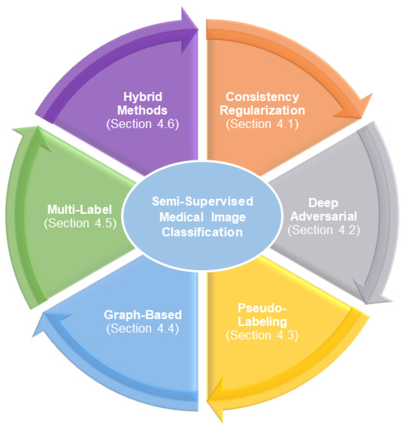
• We propose a comprehensive categorization for primary DSSL methods applied to medical image classification, categorizing these methods into six main groups. Each category is examined for variations, accompanied by standardized descriptions and unified schematic representations.
• We extensively explain each approach, frequently including important equations, elucidate the developmental context underlying the methods, and provide essential performance comparisons.
• A compilation of resources for DSSL is assembled, comprising open-source codes for several reviewed methods, well-known benchmark datasets, and performance evaluations across various label rates on these benchmark datasets.
• We pinpoint three undetermined issues and explore potential research directions for future studies, drawing insights from recent notable research in this area.

Additionally, we strive for a fairer comparison and analysis of various methods and studies showcasing datasets with accuracy for different considered semi-supervised categories. Overall, review aims to provide an extensive comparative analysis of semi-supervised methods for medical image classification task based on loss function and model design and suggesting the gaps and future recommendation for further improvement in semi-supervised techniques.

2. Background

In this section, we begin by providing an introduction to the fundamentals of DSSL. That will be followed by a through overview of state-of-the-art DSSL techniques. The Problem Formulation aspect focuses on efficiently illustrating the DSSL framework, with a specific emphasis on single-label classification tasks due to their simplicity in description and implementation. For the readers interested in multi-label classification tasks, we recommend referring to Cevikalp’s articles [30,31]. Let $D=\{D_C, D_W\}$ represent the complete dataset, comprising a small labeled subset $D_C={\{a_i, b_i\}}_{i=1}^C$ and a larger unlabeled subset $D_W={\left\{\right(a_i\left)\right\}}_{i=1}^W$, with the general assumption that $C \ll W$. The dataset is assumed to contain $K$ classes, with ${\left\{b_i\right\}}_{i=1}^C \in \left(b_i^1, b_i^2, \dots , b_i^k\right)$, where $b_i^k=1$ indicates labeling by the $k_{th}$ class, and otherwise $b_i^k=0$. Formally, SSL aims to address the optimization problem outlined below,

$$\underset{\Theta }{\min }\sum _{\left(a,b\right) \in D_c}{\mathcal{l}}_s\left(a, b,\Theta \right)+\alpha \sum _{a \in D_W}{\mathcal{l}}_u(a, \Theta )+\beta \sum _{a \in D}\mathrm{Ʀ}\left(a, \Theta \right)$$

(1)

where ${\mathcal{l}}_s$, ${\mathcal{l}}_u$, and $\mathrm{Ʀ}$ represents the per-example supervised loss (cross-entropy for classification), unsupervised loss, and regularization (consistency loss or a custom regularization term). It is worth noting that unsupervised loss terms are often not strictly distinguished from regularization terms, as the latter are typically not guided by label information. Finally, $\Theta$ represents the model parameters, while $\alpha$ and $\beta$, both belonging to $\mathrm{Ʀ}>0$, signify the trade-off.

2.1. Classification Overview

Distinct selections of architectures and variations in unsupervised loss functions or regularization terms result in diverse semi-supervised approaches. As depicted in Figure 1, we will examine these methodologies from various perspectives and frameworks. The approaches within the domain of DSSL can be categorized into five distinct research groups.

2.1.1. Consistency Regularization Methods

Consistency regularization techniques impose constraints into the loss functions based on the manifold or smoothness assumption [32,33]. These constraints are formulated using three approaches: input perturbation, weights perturbation, and layer perturbations within the network. In SSL methods, the Teacher-Student model is commonly used as the prevalent structure for consistency regularization. Section 4.1 discusses various learning models that emerge as a result of using different perturbation strategies.

2.1.2. Deep Adversarial Methods

Adversarial models like Generative Adversarial Networks (GANs) [34,35], Variational Auto-Encoders (VAEs) [36], and their derivatives have been developed to investigate the distribution of the training dataset and subsequently create novel instances [37]. While the standard GAN utilizes the Jensen-Shannon (JS) divergence to grasp the data distribution, it may encounter instability and weak signals, especially as the discriminator nears a local optimum, a situation referred to as gradient vanishing [36,37]. Larsen et al. [36] introduced a novel GAN architecture that merges a variational autoencoder (VAE) with a GAN, resulting in a VAE-GAN. This adaptation involves replacing the VAE’s decoder with a GAN generator and adjusting the loss function to be evaluated by a discriminator [37,38]. Various semi-supervised generative strategies have been explored within these frameworks. Section 4.2 will delve into a comprehensive review of these models.

2.1.3. Pseudo-Labeling Methods

The predominant strategy employed by pseudo-labeling methods involves generating labels for unlabeled instances based on high-confidence predictions of the model [39,40]. These pseudo-labels are then utilized to regulate the model training and classify these methods as bootstrapping algorithms [41,42]. However, traditional pseudo-labeling faces several challenges, including bias towards the majority class and limited adaptability to multi-label and multi-class scenarios. This is because confidence-driven pseudo-labeling tends to favor majority-class samples, leading to a biased model [43,44]. In Section 4.3 of the study, two variations of pseudo-labeling methods are explored, which are distinguished by the number of learners involved.

2.1.4. Graph-Based Methods

Graph-based SSL typically involves creating a similarity graph from the original dataset. In this graph, each node corresponds to a training example, and the weighted edges signify the similarity between pairs of nodes. By leveraging the manifold assumption, label information for unlabeled examples can be deduced from the constructed graph [45,46]. In Section 4.4, our emphasis is on examining methods for label inference in graph embedding SSL. For details on graph construction, readers are directed to Z Song’s article [47].

2.1.5. Multi-Label Methods

In a multi-label SSL system, specific labels or sets of labels are used to extract useful information from both labeled and unlabeled instances simultaneously. The system involves several steps to reduce and enrich the features to evaluate the SSL method and enhance the system’s overall performance [48,49]. Section 4.5 will explain these steps in detail, including how the labels propagate within the system.

2.1.6. Hybrid Methods

Hybrid approaches involve integrating diverse methodologies, including consistency regularization [50,51,52,53], pseudo-labeling [39,54], data augmentation [55,56,57,58,59], entropy estimation [60,61], and other elements [62,63,64], to enhance performance. In the upcoming Section 4.6, we will examine different categories of hybrid methods.

Distinguishing between generative methods and graph-based methods depends on whether new instances are created and if the construction of a graph is based on training instances and labels. The differentiation becomes challenging when considering consistency regularization and pseudo-labeling methods. Pseudo-labeling involves assigning pseudo-labels to unlabeled examples, and using them for supervised learning, while consistency regularization methods prioritize consistency constraints over pseudo-labels. Hybrid approaches often combine these concepts, with consistency regularization and pseudo-labeling being a common combination.

Table 2. Overview of DSSL techniques.

Methods	Description	Key Points
Consistency Regularization Methods	Formulating constraints on consistency	Assumptions are evident and rational; relying on the utilization of data augmentation and perturbation techniques.
Deep Adversarial Methods	Involving generative models like GAN, VAE, and their derivatives	Induce new training instances; challenging to attain optimal outcomes for both the generative and downstream task.
Pseudo-Labeling Methods	Pseudo-labeling unlabeled examples using labeled examples	Generating pseudo-labels; these labels produced artificially may contain inaccuracies.
Graph-Based Methods	Constructing graphs from training datasets and employing graph-based approaches to address subsequent tasks	Acquiring additional knowledge through graphs; dependent on effectively representing the relationships among training samples.
Multi-Label Methods	Labels or sets of labels are used to extract useful information from both labeled and unlabeled instances	Controls complexity and make smooth predictions; optimize combine methods.
Hybrid Methods	Combining different learning approaches, such as incorporating consistency regularization and employing pseudo-labeling techniques	Enhanced efficiency and resilience; increased size of the model.

summarizes the key components of these methods. In terms of the availability of test data during training, SSL can be categorized into two settings: transductive and inductive learning. Transductive learning assumes that unlabeled samples in training are the exact data to be predicted, aiming to generalize over these unlabeled samples. On the other hand, inductive learning assumes that the semi-supervised classifier learned during training remains applicable to new, unseen data.

2.2. Estimations

Test evaluations often serve as a benchmark for assessing the effectiveness of DSSL methods. However, the outcomes of these evaluations are influenced by several factors. According to A. Oliver (2018), the sensitivity of DSSL methods to the quantity of labelled and unlabeled samples varies, and the choice of implementations and training strategies significantly impacts the results [65]. Q. Xie’s (2020) article demonstrates that models with identical architecture but different parameters yield diverse test performance outcomes [66]. Additionally, permutation-invariant settings and data augmentation techniques introduce considerable variation in the experimental results, even under similar conditions. Various approaches, such as adversarial dropout, dual students, and mean teachers, exhibit distinct average runtimes, contributing to divergent results [67,68,69]. These disparities hinder direct comparisons between different methodologies.

3. Methodology

The review methodology employed in this study is grounded in referencing existing literature, facilitating the exploration of cutting-edge techniques, analyses, interpretations, and implications of DSSL in the context of image classification tasks. Following the guidelines outlined in [70,71,72], the literature review progressed through the following phases:

• Review: The primary inquiry driving the literature review was focused on conducting a comparative analysis of various DSSL techniques for medical image classification, with an emphasis on loss function and model design;
• Search: This search encompassed journal articles, conference articles, published reports, and official websites (Figure 2).

Document selection criteria included consideration of citation frequency and relevance. Scientific databases such as Science Direct, Springer, and IEEE were utilized. The primary search keywords were “medical”, “image”, and “semi-supervised”, with additional terms like “analysis” and “classification”. Specific category-related keywords, such as adversarial, consistency, GANs, multi-label, and graphs were included in the searches. Articles published between 2019 and 2024 were included, and sorting was based on relevance and citation count whenever feasible.

The selection of research articles involved an initial analysis of abstracts, followed by a comprehensive review of the articles. Research papers exclusively addressing medical image segmentation without a dedicated section on classification were omitted. Our research’s inclusion criteria were as follows:

• The primary focus of the study should be on SSL.
• Inclusion of a thorough description of the model architecture and a clear presentation of the classification algorithm’s results.
• For instance, we consider originality, significance of findings, and high number of citation factors.

On the contrary, the following were the exclusion requirements for our review article:

• There is no peer review or trustworthy records indexing for the research.
• The research has not introduced relevant augmentation or alteration to the established deep learning algorithm.
• The research provides an ambiguous explanation of the experimentation and classification results. The literature review process is delineated in the PRISMA representation depicted in Figure 3.

In contrast to the survey examining papers up to 2018, this study centers on research published between 2019 and 2024 [25]. Unlike Cheplygina et al. [25], who provided a broad survey of unsupervised and semi-supervised techniques for the analysis of medical images, this study concentrated specifically on SSL for classification tasks, offering more in-depth descriptions of the models discussed [25]. In addition, while this work distinctively focuses on application of medical image classification using deep semi-supervised learning (DSSL), diverging from the segmentation-centric analysis [73] presented in existing literature. Specifically, while the referenced study delves into DSSL applications in segmentation, highlighting strategies like pseudo labeling and noise handling, our analysis critically examines the application of DSSL techniques to classification tasks, highlighting their relevance in the early identification and treatment of patients, alongside discussing the unique challenges and future directions in this area.

4. Methods

This section presents the categorization of deep semi-supervised image classification methods, involving the integration of critical features from the two realms of semi-supervised loss function and model construction. The methods being discussed are classified into specific types, such as deep adversarial, consistency regularization, pseudo-labeling, graph-based, multi-label and hybrid methods. Each method is introduced with a description of its fundamental principles and the overall structure of its loss function. Subsequently, the improvements made to each method are presented. Finally, a summary of the outcomes reported in the original papers is provided, with a focus on their notable achievements, limitations, and potential avenues for further development.

4.1. Consistency Regularization

Consistency-based methods prompt models to generate coherent outputs even when presented with modified versions of the specific noisy Gaussian inputs [23]. More specifically, if an input ${\mathcal{x}}_i$ belongs to class $c$, then the altered input ${\mathcal{x}}_i^{\prime }$ should also be classified as belonging to class $c$. Consistency regularization stems from the smoothness hypothesis, which posits that legitimate changes to data points should not cause significant shifts in the model’s predictions [65,74,75]. The Teacher-Student configuration is the most widely used structure for consistency regularization in SSL methods. The model functions as a student by learning conventionally and simultaneously acts as a teacher to generate targets. Let ${\Theta }^{\prime }$ represent the target weight, and $\Theta$ symbolize fundamental student weights. The consistency prerequisite is expressed as

$${\mathbb{E}}_{a\in D}\mathrm{Ʀ}(f\left(\Theta , a\right), f\left({\Theta }^{\prime }, a\right), {\tau }_a)$$

(2)

where $f\left(\Theta , a\right)$ predicts the output for input $a$ and $f\left({\Theta }^{\prime }, a\right)$ represents the teacher’s predictions, which serve as the consistency targets ${\tau }_a$ for the student. $\mathrm{Ʀ}\left(-,-\right)$ scales the vector distance and is typically set as the Mean Squared Error also known as MSE or KL-divergence. The procedural methods in which diverse consistency regularization techniques formulate targets are distinctive. Enhancing the quality of ${\tau }_a$ involves strategies such as meticulous perturbation selection over additive or multiplicative noises. An alternate approach is to meticulously examine the teacher model instead of simply mimicking the student model [76]. Under consistency regularization we further discussed two main approaches: Temporal Ensemble and Mean Teacher in Section 4.1.1 and Section 4.1.2, respectively, as illustrated in Figure 4.

4.1.1. Temporal Ensemble

Temporal ensemble, as detailed in [51], is a stochastic perturbation method designed to boost $\mathsf{ᴨ}$-model computational capability [77], achieved by generating two arbitrary augmentations data with and without labels, which pass an input sample through the network multiple times [77]. This technique combines a prediction derived ${\mathit{Y}}_t$ from past iterations with a real-time perturbed prediction $\widetilde{{\mathit{Y}}_t}$ to penalize minor variations in the outputs, requiring only a single propagation for each epoch. The temporal ensemble method differs from other methods in that it focuses on aggregating previously weighted average predictions compared to relying on a single randomly augmented value, thereby enhancing the robustness of the learning process. The ensemble output’s ${\mathit{Y}}_t$ is updated using ${\mathit{Y}}_t ⃪ \alpha {\mathit{Y}}_t+(1-\alpha )\widetilde{{\mathit{Y}}_t}$ momentum term called $\alpha$ which determines the extent of the ensemble’s influence throughout the training history. Intriguingly, hyperparameters can be transformed in accordance with uncertainty in data, such as by assigning greater weights to high-confidence predictions.

To address the complexities of disentangled learning and self-ensembling within CheXpert [78] binary classification, Gyawali et al. [79] integrated a temporal ensemble alongside an unsupervised variational auto-encoder (VAE). Previous studies [80,81] employed the disentangled representation $M1$ obtained from an unsupervised VAE as an outline for a subsequently developed VAE-based semi-supervised framework, often termed the $M1+M2$ model. The authors [79] sought to refine the $M1+M2$ model by substituting $M2$ for a self-ensembling SSL network and incorporating a temporal ensemble on unsupervised targets to promote agreement among ensemble predictions. This strategy utilizes a VAE within the unsupervised learning domain to capture a dataset’s intrinsic generative characteristics. This entailed assuming that the data $D$ is generated by a likelihood function, denoted as $\mathsf{Ƥ}\Theta \left(l\right|m)$, with a latent variable $m$ possessing a prior distribution represented as $\mathsf{Ƥ}\left(m\right)$. To address the computational challenge of exact posterior inference, an introduced distribution, denoted as $\mathsf{Ƣ}\varnothing \left(m\right|l)$, was put to approximate the true posterior, $\mathsf{Ƥ}\left(m\right|l)$ through variational inference [79,82]. With regard to parameters $\Theta$ and $\varnothing$, the training of the VAE was centered on optimizing the variational evidence lower bound of the marginal probability around the training data.

$$\log \mathsf{Ƥ}\left(l\right)\ge \mathcal{L}={\mathbb{E}}_{\mathsf{Ƣ}\varnothing \left(m|l\right)}\left[\log \mathsf{Ƥ}\Theta \left(l\right|m\left)\right]-KL (\mathsf{Ƣ}\varnothing \left(m|l\right)||\mathsf{Ƥ}\left(m\right)\right)$$

(3)

The following equation’s first term seeks to minimize reconstruction error, and its second term uses the Kullback-Leibler (KL) divergence measure to adjust the learned posterior density $\mathsf{Ƣ}\varnothing \left(m\right|l)$ in incorporating a prior $\mathsf{Ƥ}\left(m\right)$. We have chosen $\mathsf{Ƥ}\left(m\right)$ to be an isotropic Gaussian, which promotes disentangled latent representations in $\mathsf{Ƣ}\varnothing \left(m\right|l)$ by encouraging independence between the latent dimensions [79,82].

For each training instance, denoted as $l^{\left(i\right)}$, ensemble predictions were derived from the VAE-learned posterior density, $\mathsf{Ƣ}\left(m^{\left(i\right)}|l^{\left(i\right)}\right)$, thereby replacing manually crafted augmentation functions with a distribution learned from unlabeled data to perturb $l^{\left(i\right)}$ [51,79]. The network incorporated dropout and temporal ensemble, accumulating predicted labels, ${\mathit{Y}}_t \mathrm{a}\mathrm{n}\mathrm{d} \widetilde{{\mathit{Y}}_t}$, after each training epoch into an ensemble output [51,79]. In each batch $B$, the network was learned to minimize the ensemble loss $\left({\mathcal{L}}^e\right)$:

$${\mathcal{L}}^e=\underset{for labeled only}{\underbrace{\frac{1}{\left|B\right|}\sum _{n ~ \left(B\cap D_c\right)}\sum _{l=1}^L\left[{-y}_{n, l} \log f\left(y_{n, p}\left|\mathsf{Ƣ}\right.\left(m\left|l\right.\right)\right)\right]}}+\underset{for labeled and unlabeled}{\underbrace{\zeta \times \frac{1}{\left|B\right|}\sum _{n ~ B}{‖{\mathit{Y}}_t-\widetilde{{\mathit{Y}}_t}‖}^2}}$$

(4)

here, the initial term corresponds to the standard cross-entropy loss and is assessed for labeled data, while the subsequent term, evaluated across all data, encouraged consensus among ensemble predictions through mean squared loss. The ramp-up weighted function for $\zeta$ initiated from zero, following the description in [51,79].

Underlying Knowledge-based Semi-Supervised Learning (UKSSL) [83] is a method for lung/colon cancer and blood cells classification, combining contrastive learning of medical visual representations (MedCLR) with an underlying knowledge-based multi-layer perceptron classifier (UKMLP) [83]. MedCLR, inspired by SimCLR [84], extracts semantic information from medical images by maximizing agreement [85] between augmented views of the same image while minimizing agreement between different images. This is facilitated by an image augmentation module $A$ and an encoder $e\left(\cdot \right)$, which employs a light transformer $LTrans$ architecture to extract semantic knowledge and produce representations $r^{\prime }$ and $r^{\prime \prime }$.

$$r^{\prime }=e\left(i^{\prime }\right)=Encoder\left(i^{\prime }\right)$$

(5)

where data transformation technique transforms the original image $i$ into two augmented images $i^{\prime }$ and $i^{\prime \prime }$. The encoder employs a $LTrans$ architecture, reshaping images into flattened 2D patches and applying linear projections and position embeddings. Multi-head self-attention (MSA) [86] and multi-layer perceptron (MLP) [87] blocks within $LTrans$ facilitate this process,

$$x_l^{\prime }=MSA\left(Norm\left(x_l-1\right)\right)+x_{i-1}$$

(6)

$$x_l=MLP \left(Norm\left(x_l^{\prime }\right)\right)+x_l^{\prime }$$

(7)

followed by a projection head $p\left(\cdot \right)$ which projects the representations $r$ to another feature space $z$ using a non-linear MLP neural network.

$$z=p\left(r\right)=W^{\left(2\right)}\sigma \left(W^{\left(1\right)}r\right)$$

(8)

The contrastive loss function $NT-Xent$ [84] optimizes the prediction task by computing the normalized temperature-scaled cross-entropy loss between positive pairs of augmented images [88,89,90]. In training, random $N$ mini-batches are sampled, augmentations $i^{\prime }$ and $i^{\prime \prime }$ applied, and images passed through the encoder $e\left(\cdot \right)$ and projection head $p\left(\cdot \right)$ to calculate similarity and update parameters.

$${\mathcal{L}}_{NT-Xent}\left(i^{\prime }, i^{\prime \prime }\right)=-\log \frac{exp\left(sim\left(z^{\prime }, z^{\prime \prime }\right)/t\right)}{{\sum }_{k=1}^{2N}\left[k\ne i\right]exp\left(sim\left(z_i, z_k\right)/t\right)}$$

(9)

The UKMLP refines feature representations learned by MedCLR using limited labeled data, with a deeper architecture comprising 12 hidden layers. Input from MedCLR is passed through these layers, with each following a rectified linear activation function $ReLU$ [83].

$$f\left(x\right)=max\left(0, x\right)$$

(10)

$$L\left(\widehat{y}, y\right)=-{\sum }_{i=1}^C{y}_i\log \left({\widehat{y}}_i\right)$$

(11)

The loss function of the UKMLP is multi-class entropy, where $\widehat{y}$ is a vector of predicted class probabilities and $y$ is a one-hot encoded vector of true class labels, computed using the natural logarithm.

4.1.2. Mean Teacher

The Temporal Ensemble method employs an exponential moving average of label predictions for individual training case and deals with deviations from this target. Nevertheless, this technique can be cumbersome when applied to large datasets because the targets are updated only once per epoch. To tackle this issue, Tarvainen and Valpola [69] introduced the Mean Teacher approach, which involves dividing the teacher model similarly to a Temporal Ensemble, with the teacher network adjusted based on the student network’s outputs. They computed the consistency cost between the teacher’s predictions and the stochastic augmentation, as well as the dropout predictions of the student. The authors referred to the ensembled prediction technique utilized in the temporal ensemble as the Exponential Moving Average (EMA). The following method evaluated the same example using an amalgam of the current and earlier iterations of the model. The teacher model weights were updated using an adaptation of the EMA method, expressed as ${\Theta }_i^{\prime }=\alpha {\Theta }_{i-1}^{\prime }+(1-\alpha ){\Theta }_i$ [91].

The Mean Teacher framework incorporates the Relation-driven Self-Ensembling Model (SRC-MT) [92] with a consistency-enforcing strategy. Additionally, SRC-MT investigates the intrinsic relationship among images, a factor often neglected in consistency-based methods like Mean Teacher. In Unsupervised analyses, the relationship between images makes it easier to extract important information from unlabeled data [93,94]. Sample Relation Consistency (SRC) is a novel paradigm introduced by SRC-MT that guarantees the consistent pattern of the relationship between the images after perturbation. In other words, if two images are similar before being disturbed, then this relationship ought to continue after the disturbance. Put more simply, there should be an identical relationship between input samples $s_1$ and $s_2$ and perturbed samples $s_1^{\prime }$ and $s_2^{\prime }$. As a result, this approach guarantees uniformity in relationships and labeling after disturbance. The framework’s general objective functions are outlined as

$$\mathfrak{L}={\mathfrak{L}}_s+\lambda {\mathfrak{L}}_u, \mathrm{where} {\mathfrak{L}}_u={\mathfrak{L}}_c+\beta {\mathfrak{L}}_{src}$$

(12)

The supervised objective in this case is represented by ${\mathfrak{L}}_s$, and the unsupervised objective, which consists of the relational consistency loss ${\mathfrak{L}}_{src}$ and the standard consistency loss ${\mathfrak{L}}_c$, is represented by ${\mathfrak{L}}_u$. The trade-off weight between supervised and unsupervised loss is represented by the parameter $\lambda$, and the hyperparameter corresponding to $\beta$ is used to balance ${\mathfrak{L}}_c$ and ${\mathfrak{L}}_{src}$.

Mean Teacher for Self-supervised and Semi-supervised Learning $\left(S^2{MTS}^2\right)$, a method for consistently classifying chest X-rays, is presented in [95]. It involves two stages of learning using the Mean Teacher framework. Using JCL, the student-teacher model is pre-trained on labelled and unlabeled data in the preliminary stage [96]. In order to establish correlations between different pairs that share a common query, this entails learning a large set of key-query pairs obtained from unlabeled data. Such a process guarantees more uniform representations for each class specific to each instance [96]. Consequently, each query ${\mathsf{ƣ}}_i$, in conjunction with numerous positive keys $k_{i, m}^{+}$, is expected to result in a minimized loss value. The loss for each pair $({\mathsf{ƣ}}_i, k_{i, m}^{+}$) is delineated as follows:

$${\mathfrak{L}}_{i, m}=-\log \left(\frac{exp\left(\frac{1}{\tau }{\mathsf{ƣ}}_i^{\top }{k}_{+, i, m}\right)}{exp\left(\frac{1}{\tau }{\mathsf{ƣ}}_i^{\top }{k}_{+, i, m}\right)}+{\sum }_{\mathcal{j}=1}^{K}exp\left(\frac{1}{\tau }{\mathsf{ƣ}}_i^{\top }{k}_{-, i, \mathcal{j}}\right)\right)$$

(13)

here, $\tau$ stands for the temperature hyperparameter, $k_{+, i, m}$ refers to the $\mathrm{m}th$ positive legend of ${\mathsf{ƣ}}_i$, and $k_{-, i, \mathcal{j}}$ denotes the, $\mathcal{j}th$ negative legend of ${\mathsf{ƣ}}_i$. The following equation calculates the total JCL loss:

$${\mathfrak{L}}_p\left({\mathfrak{D}}_X, {\Theta }_2, {\Theta }_2^{\prime }\right)=-\frac{1}{\left|{\mathfrak{D}}_X\right|}{\sum }_{i=1}^{\left|{\mathfrak{D}}_X\right|}\frac{1}{M}{\sum }_{m=1}^M\left[{\mathfrak{L}}_{i, m}\right]$$

(14)

where $M$ is the number of positive keys and ${\mathfrak{D}}_X$ is the set of labeled and unlabeled images. The second phase involves maintaining an Exponential Moving Average (EMA) while fine-tuning the pre-trained student-teacher model using the Mean Teacher approach following the equation ${\Theta }_i^{\prime }=\alpha {\Theta }_{i-1}^{\prime }+(1-\alpha ){\Theta }_i$.

NoTeacher (NoT) [97] presents a departure from the Mean Teacher methodology, where the teacher’s consistency target relies on the Exponential Moving Average (EMA) of the student. There is a close association between the weights of the student and the teacher for the reason the teacher’s weight is an ensemble of the student weights. However, this approach can create a confirmation bias, where the teacher reinforces what it already believes [68]. The NoTeacher framework uses two separate networks in place of an EMA component to solve this issue. The NoTeacher framework applies two random augmentations to an input value $x$, resulting in two new samples, $x_1$ and $x_2$. These samples are fed into two networks, $F_1$ and $F_2$, with similar architectures. For labeled inputs, the outputs are labeled as $f_1^L$ and $f_2^L$, and for unlabeled inputs, as $f_1^U$ and $f_2^U$. Next, in order to ensure prediction consistency between $F_1$ and $F_2$, a loss function is computed. The consistency loss and the supervised cross-entropy loss combine to form this loss function. The outputs $f_1$ from $x_1$ and $f_2$ from $x_2$ must be similar when $x_1$ and $x_2$, are augmented versions of the similar input $x$.

Moreover, if $x$ serves as a labeled input, it is essential for both networks to provide outputs that correspond with the target value $y$. The total loss is propagated backward to adjust the network parameters to achieve this. Both the Mean Teacher technique and the NoTeacher method use two networks with similar architectures. On the other hand, the NoTeacher approach does away with the EMA, completely separating the networks. Furthermore, NoTeacher’s loss function is based on a graphical model with $f_1$, $f_2$, and $y$ as its nodes. A consensus function called $f_c$, which is connected to every node, ensures that the outputs of the labeled and unlabeled data are consistent and fall between 0 and 1.

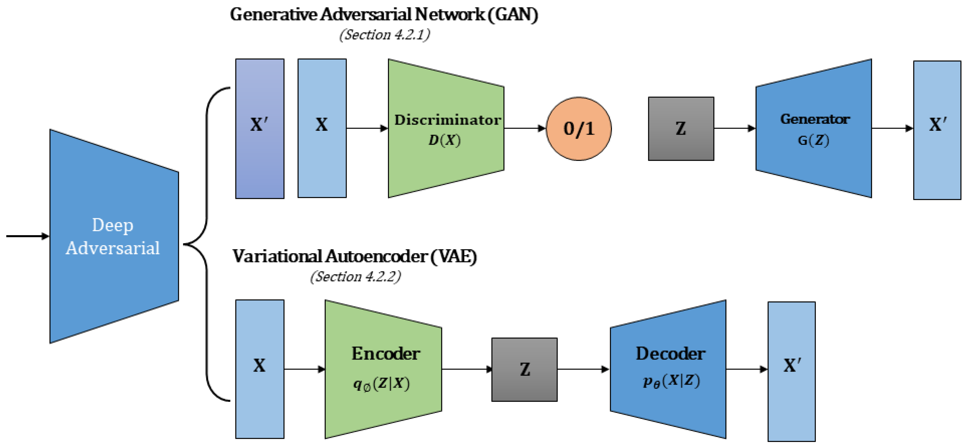
4.2. Deep Adversarial Methods

Deep adversarial models are different from discriminative models in that their primary objective is to approximate the probability distribution from which the data originates and generate similar samples [91]. Specifically, in machine-learning classification tasks, the last stage is the same as for discriminative classifiers: estimating the target variable’s conditional probability [98]. The deep adversarial semi-supervised techniques covered in this section are based on variational autoencoders (VAEs) and generative adversarial networks (GANs), as depicted in Figure 5.

4.2.1. Generative Adversarial Network (GAN)

Using a scenario involving two deep neural network models—a generator and a discriminator—Generative Adversarial Networks (GANs) [34] were constructed to demonstrate the underlying distribution within real data samples. While the discriminator serves as a binary classifier set with distinguishing real samples (from the dataset) from bogus ones (by the generator), the generator seeks to produce acceptable samples that approximate the true data distribution. Both models underwent adversarial training, similar to the two rivals who continuously hone their abilities to surpass one another in a competition. A conventional GAN [34,99] comprises a generator, denoted as $G$, and a discriminator, referred to as $d$. The objective of the generator $G$ is to learn a distribution $\rho G$ over data $a$ given a prior on input noise variables $\rho \mathfrak{z}\left(\mathfrak{z}\right)$. The generator $G$ produces fake samples $G\left(\mathfrak{z}\right)$ with the intention of deceiving the discriminator $d$. On the other hand, $d$’s goal is to distinguish actual training samples $a$ from the fake samples $G\left(\mathfrak{z}\right)$. As shown, $d$ and $G$ participate in a two-player minimax game with the value function $\mathcal{V}(G;D)$:

$$\underset{G}{\min }\underset{d}{\max }\mathcal{V}\left(G;D\right)={\mathbb{E}}_{a~\rho \left(a\right)}\left[\log d\left(a\right)\right]+{\mathbb{E}}_{{\mathfrak{z}~\rho }_{\mathfrak{z}}}\left[\log \left(1-d\left(G\right(\mathfrak{z}\left)\right)\right)\right]$$

(15)

Since GANs have the ability to learn the distribution of accurate data from unlabeled samples, which makes them useful in semi-supervised learning (SSL). In SSL scenarios, various approaches leverage GANs, and one effective method involves combining an unsupervised GAN value function with a supervised classification objective function, such as ${\mathbb{E}}_{(a, b)ϵ{\mathcal{X}}_{\mathrm{l}}}\left[\log d\left(b\right|a)\right]$. In this approach, GANs are used to generate new data points that are similar to the actual data. The subsequent discussion reviews several notable methods in the realm of semi-supervised GANs.

SS-DCGAN, as described in [100], is designed for retinal image synthesis and glaucoma detection, drawing from the DCGAN architecture [101]. It improves upon Vanilla GAN [102,103,104] by incorporating strided convolutions in the discriminator, fractional-strided convolutions in the generator, batch normalization in both networks, replacing fully connected layers with average pooling, utilizing $ReLU$ activation in the generator (excluding the output), and $LeakyReLU$ activation in the discriminator. Specifically, one change is to the final output layer of $D$, which has three neurons for glaucoma classifier training and one neuron for synthesis. $D$ therefore, acts as a classifier, assigning as normal, glaucoma, or synthetic category to each sample. The loss function of the method was defined as follows:

$${\mathcal{L}=\mathcal{L}}_{supervised}+{\mathcal{L}}_{unsupervised}$$

(16)

$${\mathcal{L}}_{supervised}=-{\mathbb{E}}_{x, y ~ {\rho }_{data}} \left(x, y\right)\log \left(\left({\rho }_{model} \left(y|x, y\right)<K+1\right)\right)$$

(17)

$${\mathcal{L}}_{unsupervised}=-\left\{{\mathbb{E}}_{x ~ {\rho }_{data} \left(x\right) }\log D\left(x\right)+{\mathbb{E}}_{\mathcal{z}~{\rho }_z\left(\mathcal{z}\right)}\log \left(1-D\left(G\left(\mathcal{z}\right)\right)\right)\right\}$$

(18)

where $K_{classes}$, ${\mathcal{L}}_{supervised}$ represents the cross-entropy loss function. Meanwhile, ${\mathcal{L}}_{unsupervised}$ corresponds to GAN’s two-player minimax game. Here, $D\left(x\right)$ denotes the likelihood of $x$ belonging to actual data, and $G\left(\mathcal{z}\right)$ represents the likelihood of $\mathcal{z}$ originating from the generator.

A supervised classification network $C$ and a reconstruction network $R$, are components of the GAN-based Semi-supervised Adversarial Classification (SSAC) [105] technique. Learnable transition layers $\left(T\right)$ facilitate the transfer of $R\prime s$ acquired image representation skills to $C$. $R$ is an adversarial autoencoder-based unsupervised network made up of a discriminator $D$ and a generator $G$. $G\prime s$ encoder and decoder produce reconstructed patches with a $64\times 64$ size, and $D$ is a four-layer deep convolutional neural network [106]. $C$ is composed of two parts: a fully connected layer with two neurons, divided by a global average pooling (GAP) layer, and an encoder resembling the one in $R$. It is significant to remember that $R$ and $C$ do not share any parameters. Each learnable $T$ layers in $C$ consists of a $1\times 1$ convolutional layer that transfers the feature maps obtained by $R$ to corresponding blocks. $R$ underwent pre-training on both labeled and unlabeled data during experimentation, whereas $C$ received pre-training on ImageNet. This is how the loss function is defined:

$${\mathcal{L}}_{SSAC}\left({\mathbb{X}}_m\right)={\mathsf{\lambda }}_1\left\{mse\left(G\left({\mathbb{X}}_m\right), {\mathbb{X}}_m\right)-\left[bce\left(D\left(G\left({\mathbb{X}}_m\right)\right), 0\right)+bce\left(D\left({\mathbb{X}}_m\right), 1\right)\right]\right\}+bce \left(C\left({\mathbb{X}}_m\right), {\mathbb{Y}}_m\right)$$

(19)

within this context, the variable ${\mathbb{X}}_m$ signifies the $m^{th}$ input sample, while ${\mathsf{\lambda }}_1$ serves as a weighting factor. The components of the function correspond to the mean squared reconstruction loss incurred by $G$, the adversarial cross-entropy loss associated with $D$, and the supervised classification loss.

Bi-Modality Medical Image Synthesis Incorporating two or more imaging modalities into a single examination is known as using SSL Sequential GANs [107,108]. This is made possible by combining multiple techniques, including positron emission tomography (PET), magnetic resonance imaging (MRI), and single photon emission computed tomography (SPECT), which use optical, magnetic, and radioactive elements to detect anomalies in the brain. Peta-SPECT and PET-CT are two types of bi-modal images [108]. Yang and colleagues have presented a model that uses GANs to produce high-quality bi-modal medical images [107]. This is performed by establishing two sequential generative networks, each dedicated to a specific modality. The first modality is automatically identified by a complexity measuring algorithm, which also provides a foundation for streamlining the development of the second, more complex modality. The process of producing the second modality is aided by training on the first modality. The generator network is trained via SSL to produce realistic images across a diverse range. The supervised learning approach involves understanding the joint distribution of various modalities, whereas the unsupervised learning approach focuses on learning the marginal distribution of modalities through adversarial learning. The architecture of the generator is as follows: a real image of a modality is first encoded into a low-dimensional latent vector, which is subsequently decoded to produce a synthetic image of the same modality. Using data from the previously generated image of the first modality, an image-to-image translator is used for the second modality to create an artificial image. Pairs of the original images are given during the supervised training. As a result, for each pair of artificial images generated by the generator, the matching pair from the original dataset can be found. As a result, pixel-wise re-construction loss serves as the foundation for the loss function in supervised training.

$${\mathcal{L}}_1={\mathbb{E}}_{\left(I_1, I_2\right) ~ \rho \left(I_1, I_2\right)}\left[{‖I_1-{\widehat{I}}_1‖}^2+{‖I_2-{\widehat{I}}_2‖}^2\right]$$

(20)

where ${\widehat{I}}_1$ and ${\widehat{I}}_2$ refer to the synthetic images, whereas $I_1$ and $I_2$ denote the genuine images. The term $‖x-\widehat{x}‖$ signifies the average Manhattan distance between the intensities of images $x$ and $\widehat{x}$, calculated pixel by pixel. Significant overfitting can affect a supervised learning model because labeled images are not readily available. Consequently, an unsupervised learning model is also applied, whereby the generator is trained with noise vectors and unpaired images rather than encodings. This model aims to reduce the Wasserstein distances between the artificial and real images [109,110,111]. Thus, the unsupervised generator’s loss function can be expressed as follows:

$${\mathcal{L}}_{unsup}={\mathit{W}}_1\ast \mathit{X}+{\mathit{W}}_2\ast \mathit{Y}$$

(21)

the variables ${\mathit{W}}_1$ and ${\mathit{W}}_2$ represent the distance between actual and synthetic images of two different modalities, with $\mathit{X}$ and $\mathit{Y}$ as additional variables. The generator is trained in a semi-supervised manner using paired training images to initiate the training process. In the following iteration, the decoder and image translator are trained in unsupervised way using unpaired images. This alternating pattern of supervised and unsupervised training has 40,000 iterations. The model uses supervised learning to generate precisely paired images, and unsupervised training to boost diversity and realism. Each image pair was classified as either clinically significant (CS) or non-CS. The generated images were used as real training data in a task that classified prostate cancer using a single label.

The technique known as Uncertainty-Guided Virtual Adversarial Training with Batch Nuclear-Norm Optimization [112] was designed to address overfitting on labeled data and enhance the discriminative power and diversity of the model. This technique integrates batch nuclear-norm (BNN) optimization [113], which, as proposed by Cui et al. [113] calculates the nuclear-norm ${‖\mathcal{P}\left(\Theta \right)‖}_{\ast }$ of the $m\times n$ prediction matrix $\mathcal{P}\left(\Theta \right)$:

$${‖\mathcal{P}\left(\Theta \right)‖}_{\ast }=\sum k=1^m\sum l=1^n {\sigma }_{k, l}\left(\mathcal{P}\left(\Theta \right)\right)$$

(22)

The expression ${\sigma }_{k, l}\left(\mathcal{P}\left(\Theta \right)\right)$ represents to the $l^{th}$ largest singular value of the matrix $\mathcal{P}\left(\Theta \right)$. The two main objectives of incorporating BNN optimization are to improve generalization and prevent overfitting on labeled data. This is accomplished by maximizing the BNN loss of the batch containing the unlabeled data and minimizing the BNN loss of the labeled data. Thus, the labeled BNN loss ${\mathcal{L}}_{lBNN}$ and the unlabeled BNN loss ${\mathcal{L}}_{uBNN}$ have the following definitions:

$${\mathcal{L}}_{lBNN}=\raisebox{1ex}{${\alpha }_l$}\!\left/ \!\raisebox{-1ex}{$B_l$}\right.{‖{\mathcal{P}}_l\left(\Theta \right)‖}_{\ast }$$

(23)

$${\mathcal{L}}_{uBNN}=-\raisebox{1ex}{${\alpha }_u$}\!\left/ \!\raisebox{-1ex}{$B_u$}\right.{‖{\mathcal{P}}_u\left(\Theta \right)‖}_{\ast }$$

(24)

The labeled and unlabeled dataset sizes are represented by the variables $B_l$ and $B_u$, respectively, and the nuclear norm of the labeled and unlabeled prediction matrices is indicated by ${‖{\mathcal{P}}_l\left(\Theta \right)‖}_{\ast }$ and ${‖{\mathcal{P}}_u\left(\Theta \right)‖}_{\ast }$, respectively. The proposed model incorporates a BNN and uncertainty guidance during the computation of the VAT loss to exclude unlabeled samples near the decision boundary. To ensure reliable learning objectives, the uncertainty ${\mathcal{U}}_{\mathcal{i}}$ is computed for each unlabeled sample ${\mathcal{X}}_{\mathcal{U}}^{\mathcal{i}}$ in a batch. The high degree of uncertainty predictions is then eliminated.

$$U_{\mathcal{i}}=-\sum _{\mathcal{j}=1}^{\mathcal{c}}{\mathcal{P}}_{\mathcal{i},\mathcal{j}}^{\mathcal{U}}\log \left({\mathcal{P}}_{\mathcal{i},\mathcal{j}}^{\mathcal{U}}\right),\mathcal{i} \in 1\dots B_{\mathcal{U}}$$

(25)

The model is trained using multiple loss functions, with ${\mathcal{P}}_{\mathcal{i},\mathcal{j}}^{\mathcal{U}}$ to representing the predicted probability of ${\mathcal{X}}_{\mathcal{U}}^{\mathcal{i}}$ for the ${\mathcal{j}}^{th}$ category and $\mathcal{c}$ denoting the total number of classes. These include the losses ${\mathcal{L}}_{bayes}^l$ and ${\mathcal{L}}_{bayes}^{\mathcal{U}}$ from the BNN, the cross-entropy loss from the supervised model ${\mathcal{L}}_{cls}$, the VAT loss derived from labeled data ${\mathcal{L}}_{vat}^l$, the VAT loss guided by uncertainty computed from unlabeled data ${\tilde{\mathcal{L}}}_{vat}^{\mathcal{U}}$. The culmination of all losses calculated over this labeled data is the comprehensive loss for labeled data:

$${\mathcal{L}}_l={\mathcal{L}}_{cls}+{\mathsf{\lambda }}_{vat}{\mathcal{L}}_{vat}^l+{\mathsf{\lambda }}_{bayes}^l{\mathcal{L}}_{bayes}^l$$

(26)

Likewise, the loss for unlabeled data can be determined in the following manner:

$${\mathcal{L}}_{\mathcal{U}}={\mathsf{\lambda }}_{vat}{\tilde{\mathcal{L}}}_{vat}^{\mathcal{U}}+{\mathsf{\lambda }}_{bayes}^{\mathcal{U}}{\mathcal{L}}_{bayes}^{\mathcal{U}}$$

(27)

where ${\mathsf{\lambda }}_{vat}$, ${\mathsf{\lambda }}_{bayes}^l$, and ${\mathsf{\lambda }}_{bayes}^{\mathcal{U}}$ represent the weighting coefficients. The primary objective function involves summing up both the supervised and unsupervised losses, ${\mathcal{L}}_l+{\mathcal{L}}_{\mathcal{U}}$.

$Cycle\mathrm{G}\mathrm{A}\mathrm{N}$ architecture [114] is a network that can translate images from one domain to another, even when there is no direct pairing between them [16]. The framework employs a GAN, which consists of two generators, ${\mathcal{G}}_{\mathsf{A}\mathsf{B}}$ and ${\mathcal{G}}_{\mathsf{B}\mathsf{A}}$. These generators are responsible for learning mappings between the domains $\mathbb{A}=\mathrm{W}\mathrm{L}\mathrm{I}$ and $\mathbb{B}=\mathrm{N}\mathrm{B}\mathrm{I}$, where ${\mathcal{G}}_{\mathsf{A}\mathsf{B}}$ maps $\mathbb{A}$ to $\mathbb{B}$ and ${\mathcal{G}}_{\mathsf{B}\mathsf{A}}$ maps $\mathbb{B}$ to $\mathbb{A}$. In addition, two discriminators, ${\mathcal{D}}_{\mathsf{A}}$ and ${\mathcal{D}}_{\mathsf{B}}$, are trained to differentiate between real and factious images from each domain. The model uses three primary losses to optimize the training process: adversarial loss ${\mathcal{L}}_{adv}$, cycle consistency loss ${\mathcal{L}}_{cyc}$, and similarity loss ${\mathcal{L}}_{sim}$.

The loss term ${\mathcal{L}}_{cyc}$, referred to as the cycle loss, is expressed as follows

$${\mathcal{L}}_{cyc}\left({\mathcal{G}}_{\mathcal{p}\mathcal{q}}, {\mathcal{G}}_{\mathcal{q}\mathcal{p}}, {\mathcal{X}}_{\mathcal{p}}\right)=\mathbb{E}\left[‖{\mathcal{X}}_{\mathcal{p}}-{\mathcal{G}}_{\mathcal{q}\mathcal{p}}\left({\mathcal{G}}_{\mathcal{p}\mathcal{q}}\left({\mathcal{X}}_{\mathcal{p}}\right)\right)‖\right]$$

(28)

the indices $\mathcal{p}$ and $\mathcal{q}$ represent the original image domain and translated domain, respectively. The adversarial loss for each generator, ${\mathcal{G}}_{\mathcal{p}\mathcal{q}}$, and discriminator, ${\mathcal{D}}_{\mathcal{p}}$, is denoted by the term $\mathcal{L}$.

$${\mathcal{L}}_{adv}\left({\mathcal{G}}_{\mathcal{p}\mathcal{q}}, {\mathcal{D}}_{\mathcal{p}}\right)={\mathbb{E}}_{{\mathcal{X}}^{\mathcal{p}}}\left[\log \left({\mathcal{D}}_{\mathcal{p}}\left({\mathcal{X}}^{\mathcal{p}}\right)\right)\right]+{\mathbb{E}}_{{\mathcal{X}}^{\mathcal{p}}}\left[\log \left(1-{\mathcal{D}}_{\mathcal{p}}\left({\mathcal{G}}_{\mathcal{q}}\left({\mathcal{X}}^{\mathcal{p}}\right)\right)\right)\right]$$

(29)

To maintain the intricate details, such as capillaries and inner blood vessels, which are vital for accurate diagnosis and specific to each image domain’s pathology, we incorporate a similarity loss, denoted as ${\mathcal{L}}_{sim}$, to complement the cycle-consistency network. The loss is defined as follows:

$${\mathcal{L}}_{sim}\left({\mathcal{G}}_{\mathsf{A}\mathsf{B}}, {\mathcal{G}}_{\mathsf{B}\mathsf{A}}\right)=\left[1-{\sum }_{\mathcal{i}}\mathsf{N}\mathsf{F}\left({\widehat{\mathcal{X}}}_{\mathsf{A}}^{\mathcal{i}}, {\mathcal{G}}_{\mathsf{A}\mathsf{B}}\left({\mathcal{X}}_{\mathsf{A}}^{\mathcal{i}}\right)\right)\right]+\left[1-{\sum }_{\mathcal{i}}\mathsf{N}\mathsf{F}\left({\widehat{\mathcal{X}}}_{\mathsf{B}}^{\mathcal{i}}, {\mathcal{G}}_{\mathsf{B}\mathsf{A}}\left({\mathcal{X}}_{\mathsf{B}}^{\mathcal{i}}\right)\right)\right]$$

(30)

here, ${\mathcal{X}}_{\mathsf{A}}\in \mathbb{A}$ and ${\mathcal{X}}_{\mathsf{B}}\in \mathbb{B}$ represent images from domains 𝔸 and 𝔹, respectively, where ${\mathcal{i}}^{th}$ denotes the index over a set of $\mathsf{N}$ elements. The images translated by the generators are denoted by ${\widehat{\mathcal{X}}}_{\mathsf{A}}$ and ${\widehat{\mathcal{X}}}_{\mathsf{B}}$. The function $\mathcal{F}\left(\mathcal{X}, \widehat{\mathcal{X}}\right)$ measures the structural similarity (SSIM) between images $\mathcal{X}$ and $\widehat{\mathcal{X}}$, as proposed in [115] and defined as:

$$\mathcal{F}\left(\mathcal{X}, \widehat{\mathcal{X}}\right)=\frac{\left({2\mathit{\mu }}_{\mathcal{X}}{\mathit{\mu }}_{\widehat{\mathcal{X}}}+{\mathcal{c}}_1\right)\left({2\mathit{\sigma }}_{\mathcal{X}\widehat{\mathcal{X}}}+{\mathcal{c}}_2\right)}{\left({\mathit{\mu }}_{\mathcal{X}}^2+{\mathit{\mu }}_{\widehat{\mathcal{X}}}^2+{\mathcal{c}}_1\right)\left({\mathit{\sigma }}_{\mathcal{X}}^2+{\mathit{\sigma }}_{\widehat{\mathcal{X}}}^2+{\mathcal{c}}_2\right)}$$

(31)

The covariance between $\mathcal{X}$ and $\widehat{\mathcal{X}}$ is denoted by ${\mathit{\sigma }}_{\mathcal{X},\widehat{\mathcal{X}}}$,

$${\mathit{\sigma }}_{\mathcal{X},\widehat{\mathcal{X}}}=\frac{1}{m-1}{\sum }_{\mathcal{j}=1}^m\left({\mathcal{X}}_{\mathcal{j}}-{\mathit{\mu }}_{\mathcal{X}}\right)\left({\widehat{\mathcal{X}}}_{\mathcal{j}}-{\mathit{\mu }}_{\widehat{\mathcal{X}}}\right)$$

(32)

where $m$ represents the number of pixels, ${\mathcal{X}}_{\mathcal{j}}$, and ${\widehat{\mathcal{X}}}_{\mathcal{j}}$ denote the ${\mathcal{j}}^{th}$ pixel of $\mathcal{X}$ and $\widehat{\mathcal{X}}$, respectively. Additionally, ${\mathit{\mu }}_{\mathcal{X}}$, ${\mathit{\mu }}_{\widehat{\mathcal{X}}}$, ${\mathit{\sigma }}_{\mathcal{X}}$, and ${\mathit{\sigma }}_{\widehat{\mathcal{X}}}$ represent the mean intensities and standard deviations of $\mathcal{X}$ and $\widehat{\mathcal{X}}$, while ${\mathcal{c}}_1$ and ${\mathcal{c}}_2$ are stabilization constants used to prevent singularities when ${\mathit{\mu }}_{\mathcal{X}}^2+{\mathit{\mu }}_{\widehat{\mathcal{X}}}^2 \approx 0$ and ${\mathit{\sigma }}_{\mathcal{X}}^2+{\mathit{\sigma }}_{\widehat{\mathcal{X}}}^2 \approx 0$ are close to zero.

The main objective of the generative network is to minimize the overall objective function, which is formulated as follows:

$$\begin{array}{c}\mathcal{L}\left({\mathcal{G}}_{\mathsf{A}\mathsf{B}},{\mathcal{G}}_{\mathsf{B}\mathsf{A}},{\mathcal{D}}_{\mathsf{A}}, {\mathcal{D}}_{\mathsf{B}}\right)\hfill \\ \hspace{1em}\hspace{1em}\hspace{1em}\hspace{1em}\hspace{1em}\hspace{1em}\hspace{1em}={\mathcal{L}}_{adv}\left({\mathcal{G}}_{\mathsf{A}\mathsf{B}}, {\mathcal{D}}_{\mathsf{A}}\right)+{\mathcal{L}}_{adv}\left({\mathcal{G}}_{\mathsf{B}\mathsf{A}}, {\mathcal{D}}_{\mathsf{B}}\right)+{\mathsf{\lambda }}_1{\mathcal{L}}_{sim}\left({\mathcal{G}}_{\mathsf{A}\mathsf{B}}, {\mathcal{G}}_{\mathsf{B}\mathsf{A}}\right)\hfill \\ \hspace{1em}\hspace{1em}\hspace{1em}\hspace{1em}\hspace{1em}\hspace{1em}\hspace{1em}+{\mathsf{\lambda }}_2{\mathcal{L}}_{sim}\left({\mathcal{G}}_{\mathsf{A}\mathsf{B}}, {\mathcal{G}}_{\mathsf{B}\mathsf{A}}\right)+{\mathsf{\lambda }}_3{\mathcal{L}}_{cyc}\left({\mathcal{G}}_{\mathsf{A}\mathsf{B}}, {\mathcal{G}}_{\mathsf{B}\mathsf{A}},{\mathcal{X}}_{\mathsf{A}}\right)\hfill \\ \hspace{1em}\hspace{1em}\hspace{1em}\hspace{1em}\hspace{1em}\hspace{1em}\hspace{1em}+{\mathsf{\lambda }}_4{\mathcal{L}}_{cyc}\left({\mathcal{G}}_{\mathsf{B}\mathsf{A}},{\mathcal{G}}_{\mathsf{A}\mathsf{B}},{\mathcal{X}}_B\right)\hfill \end{array}$$

(33)

where ${\mathsf{\lambda }}_{\mathcal{i}}$ is a hyperparameter used to balance the impact of the losses. The generators aim to minimize this function, while the discriminators aim to maximize it.

4.2.2. Variational Autoencoder (VAE)

Adaptable models called variational autoencoders (VAEs) [82,116] generative latent-variable models in conjunction with deep autoencoders. Instead of directly modeling the observations of the dataset, the generative model captures representations of the underlying distributions. $\mathcal{p}\left(\mathcal{x},\mathcal{z}\right)=\mathcal{p}\left(\mathcal{z}\right)\mathcal{p}\left(\mathcal{x}|\mathcal{z}\right)$, is the expression used to express the joint distribution, where $\mathcal{p}\left(\mathcal{z}\right)$ is a prior distribution over the latent variables $\mathcal{z}$. A variational approximation $\mathcal{q}\left(\mathcal{z}|\mathcal{x}\right)$ to the posterior $\mathcal{p}\left(\mathcal{z}|\mathcal{x}\right)$ is constructed by an encoder, and a decoder parameterizes the likelihood $\mathcal{p}\left(\mathcal{x}|\mathcal{z}\right)$. This is the two-stage network architecture of VAEs. The evidence lower bound, or $ELBO$, can be stated as follows. The variational approximation of the posterior seeks to maximize the marginal likelihood:

$$\log p\left(x\right)=\log {\mathbb{E}}_{\mathcal{q}\left(\mathcal{z}|\mathcal{x}\right)}\left[\frac{\mathcal{p}\left(\mathcal{z}\right)\mathcal{p}\left(\mathcal{x}|\mathcal{z}\right)}{\mathcal{q}\left(\mathcal{z}|\mathcal{x}\right)}\right]\ge {\mathbb{E}}_{\mathcal{q}\left(\mathcal{z}|\mathcal{x}\right)}\left[\log \frac{\mathcal{p}\left(\mathcal{z}\right)\mathcal{p}\left(\mathcal{x}|\mathcal{z}\right)}{\mathcal{q}\left(\mathcal{z}|\mathcal{x}\right)}\right]$$

(34)

In the upcoming section, we will examine several substantial latent variable techniques employed in medical image classification through SSL.

$MAVEN$ architecture [117] advances the field by combining image generation and classification, drawing inspiration from Variational Autoencoder (VAE) [82,116] and Generative Adversarial Network (GAN) models [34,118,119]. While VAE employs an encoder $E$ and decoder $D\prime$ for explicit image generation, GAN operates with a generator $G$ and discriminator $D$ in a competitive learning setup to enhance performance over training data. VAE-GANs, which integrate $D\prime$ and $G$, have the potential to merge these networks because they both produce data from the representation $\mathcal{z}$, as introduced by Makhzani et al. [120]. $E$, $G$, and $D$, are the CNNs that make up $MAVEN$; they are implemented with either convolutional or transposed convolutional layers. To create representation $\mathcal{z}\left(\mathcal{x}\right)$. $E$ first reduces the dimensionality of true samples $\mathcal{x}$. Next, $G$ generates generated samples by sampling noise $\mathcal{z}\left(\mathcal{x}\right)~ {\mathcal{q}}_{\mathsf{\lambda }}\left(\mathcal{x}\right)$, or importing noise samples from distribution $\mathcal{z}~{\mathcal{p}}_{\mathcal{g}}\left(\mathcal{z}\right)$. $D$ assesses inputs from real unlabeled, labeled, and generated data distributions. $G$ uses fractionally stridden convolutions to extract the latent code and modify the image dimension.

In $MAVEN$, the integration of $VAE-GAN$ extends to incorporate numerous discriminators grouped in an ensemble layer. $K$ discriminators are pooled together, and the combined feedback

$$V\left(D\right)=\frac{1}{K}{\sum }_{\mathcal{k}=1}^K{\mathcal{w}}_{\mathcal{k}}{D}_{\mathcal{k}}$$

(35)

is conveyed to $G$. A single discriminator is arbitrarily chosen to introduce variability in feedback from considerable discriminators.

To support training for an $\mathcal{n}-class$ classifier, $D$ assumes an additional role as an $(\mathcal{n}+1)-classifier$. A SoftMax function is used to generate multiple logits instead of the sigmoid function. This allows $D$ to take an image $\mathcal{x}$ as input and produce an $\left(\mathcal{n}+1\right)-dimensioanl$ vector of logits $\left\{{\mathcal{l}}_1, \dots , {\mathcal{l}}_{\mathcal{n}}, {\mathcal{l}}_{\mathcal{n}+1}\right\}$. The generated data is represented by the $\left(\mathcal{n}+1\right)$ class, and these logits are then converted into class probabilities for the $\mathcal{n}$ labels in the true data. The probability that the observation $\mathcal{x}$ is true and falls within class 1 for each $1 \le \mathcal{i}\le \mathcal{n}$,

$$\mathcal{p}\left(\mathcal{y}=\mathcal{i}|\mathcal{x}\right)=\frac{exp\left({\mathcal{l}}_{\mathcal{i}}\right)}{{\sum }_{\mathcal{j}=1}^{\mathcal{n}+1}exp\left({\mathcal{l}}_{\mathcal{i}}\right)}$$

(36)

whereas the likelihood that $\mathcal{x}$ is generated corresponds to $\mathcal{i}=\mathcal{n}+1$.

Both supervised and unsupervised losses are included in $D\prime s$ loss function. The model employs the conventional supervised learning loss when it is given appropriately labeled data. However, the unsupervised loss includes the original $GAN loss$ for true and generated data from two sources: directly from $G$ and through $G$ from $E$, when it receives unlabeled data from three different sources.

$${\mathcal{L}}_{D_{supervised}}=-{\mathbb{E}}_{\mathcal{x},\mathcal{y}~{\mathcal{p}}_{data}}\log \left[\mathcal{p}\left(\mathcal{y}=\mathcal{i}|\mathcal{x}\right)\right], \mathcal{i}<\mathcal{n}+1$$

(37)

In $G\prime s$ instance, the initial $GAN loss$ and the feature loss are applied simultaneously. The total $G loss$ is made up of the cost of maximizing the $log probability$ of $D$ making an error on the generated data as well as the combined feature loss.

$${\mathcal{L}}_{G_{feature}}={‖{\mathbb{E}}_{\mathcal{x}~{\mathcal{p}}_{data}}f\left(\mathcal{x}\right)-{\mathbb{E}}_{\widehat{\mathcal{x}} ~ G}f\left(\widehat{\mathcal{x}}\right)‖}_2^2$$

(38)

When using the encoder $E$, maximizing the $ELBO$ is the same as minimizing the Kullback-Leibler (KL) divergence and helps to make approximate posterior inferences. To guarantee that the features of the data match the actual distribution of the data, the loss function incorporates both a feature loss and the KL divergence.

$${\mathcal{L}}_{E_{KL}}=-KL\left[{\mathcal{q}}_{\mathsf{\lambda }}\left(\mathcal{z}|\mathcal{x}\right)‖\mathcal{p}\left(\mathcal{z}\right)\right]={\mathbb{E}}_{{\mathcal{q}}_{\mathsf{\lambda }}\left(\mathcal{z}|\mathcal{x}\right)}\left[\log \frac{\mathcal{p}\left(\mathcal{z}\right)}{{\mathcal{q}}_{\mathsf{\lambda }}\left(\mathcal{z}|\mathcal{x}\right)}\right] \approx {\mathbb{E}}_{{\mathcal{q}}_{\mathsf{\lambda }}\left(\mathcal{z}|\mathcal{x}\right)}$$

(39)

SVAEMDA approach [121] presents a novel predictor employing a variational autoencoder framework to forecast connections between diseases and miRNAs [122,123,124]. This model, a variant of autoencoder [82,125] stemming from variational Bayesian and probabilistic graphical models, creates an estimated posterior probability distribution ${\mathcal{p}}_{\mathsf{\Phi }}\left(\mathcal{z}|\mathcal{x}\right)$ via its encoder, diverging from a predetermined latent vector. Following this, the decoder employs samples from said distribution to restore the input data, yielding the probability of reconstruction ${\mathcal{p}}_{\Theta }\left(\mathcal{x}|\mathcal{z}\right)$. Here, $\mathsf{\Phi }$ and $\Theta$ characterize the parameters governing the encoder and decoder, respectively.

The marginal likelihood of the VAE model, represented as $\mathcal{L}(X, X^{\prime })$, is calculated by summing the marginal log-likelihoods across all observed samples, which can be written as:

$$\mathcal{L}\left(X, X^{\prime }\right)={\sum }_{\mathcal{i}=1}^N\log {\mathcal{p}}_{\Theta }\left({\mathcal{x}}_{\mathcal{i}}\right)$$

(40)

where $N$ signifies the count of training samples (established miRNA-disease associations), $\mathcal{x}$ represents an individual sample, and $X^{\prime }$ refers to the $VAE$ output. The marginal log-likelihood of each sample, $\log {\mathcal{p}}_{\Theta }\left(\mathcal{x}\right)$, is characterized as:

$$\log {\mathcal{p}}_{\Theta }\left(\mathcal{x}\right)=D_{KL}\left({\mathcal{q}}_{\mathsf{\Phi }}\left(\mathcal{z}|\mathcal{x}\right)‖{\mathcal{p}}_{\Theta }\left(\mathcal{z}|\mathcal{x}\right)\right)+\mathcal{L}\left(\Theta , \mathsf{\Phi };\mathcal{x}\right)$$

(41)

The initial part of the equation represents the KL divergence between the approximate and true posteriors, while the subsequent part denotes the variational lower bound of $\log \mathcal{p}\left(\mathcal{x}\right)$, with ${\mathcal{p}}_{\Theta }\left(\mathcal{z}\right)$ serving as the prior distribution. By employing a reparameterization technique, the $VAE$ renders the loss function differentiable and amenable to optimization through stochastic gradient methods. This technique involves transforming $\mathcal{z}$ as $\mathcal{z}=\mu +\sigma \odot \in$, where $\in$ is sampled from a normal distribution with mean $0$ and standard deviation $1$, while $\mu$ and $\sigma$ denote the mean and standard deviation parameters of ${\mathcal{q}}_{\mathsf{\Phi }}\left(\mathcal{z}|\mathcal{x}\right)$, respectively, and $\odot$ signifies the Hadamard product. Finally, the lower bound of the marginal log-likelihood is approximated as:

$$\mathcal{L}\left(\Theta , \mathsf{\Phi };\mathcal{x}\right)\approx -D_{KL}\left({\mathcal{q}}_{\mathsf{\Phi }}\left(\mathcal{z}|\mathcal{x}\right)‖{\mathcal{p}}_{\Theta }\left(\mathcal{z}\right)\right)+\frac{1}{L}{\sum }_{\mathcal{l}=1}^{\mathcal{L}}\log {\mathcal{p}}_{\Theta }\left(\mathcal{x}|{\mathcal{z}}_{\mathcal{l}}\right)$$

(42)

where $\mathcal{L}$ represents the number of samples drawn for $\mathcal{z}$, and the computation of the first term on the right-hand side follows the methodology outlined by Kingma et al. [82].

Robust predictive model SCAN [126], integrating a Bayesian variational autoencoder, has been developed for predicting cancer prognosis. SCAN consists of a microarray $VAE$ and a multimodal classifier. The microarray $VAE$ acquires concise gene profile representations and enables SSL by integrating untagged patient data. Furthermore, SCAN encompasses microarray and clinical classifiers, each followed by a standard output layer to generate predictions. The multimodal classifier manages both microarray and clinical data, with weighted outputs merged to generate the ultimate prediction.

The equation for the shared output layer is represented as:

$${\widehat{\mathcal{y}}}_i=\sigma \left(1_{\mathcal{x}}\odot {\mathcal{w}}_{\mathcal{x}}^T\cdot O_{\mathcal{x}}+1_{\mathcal{C}}\odot {\mathcal{w}}_{\mathcal{C}}^T\cdot O_{\mathcal{C}}\right),\mathcal{i}=1, 2$$

(43)

Here, $O_{\mathcal{x}}$ and $O_{\mathcal{C}}$ denote the outputs from microarray and clinical classifiers, respectively. ${\mathcal{w}}_{\mathcal{x}}$ and ${\mathcal{w}}_{\mathcal{C}}$ represent the corresponding weights, $\odot$ denotes the element-wise product, and $\sigma \left(\cdot \right)$ is the sigmoid function. The indicator functions $1_{\mathcal{x}}$ and $1_{\mathcal{C}}$ ensure that the weighted vote takes into account either microarray or clinical data, enabling patients with or without missing clinical features to contribute to predictions. For $Type I$ patients, predictions are the average of ${\widehat{\mathcal{y}}}_1$ and ${\widehat{\mathcal{y}}}_2$. For other types, predictions directly come from ${\widehat{\mathcal{y}}}_i$ obtained from the available subnetwork classifier. Lower bounds for $Type II$ and $III$ patients are calculated differently in the microarray $VAE$.

The complete loss function $\mathcal{L}$ encompasses lower bounds representing data generation probabilities for various patient categories, in addition to an auxiliary loss function $BCE$ specifically for $Type I$ patients. Subsequently, the model’s loss function is iteratively refined through back-propagation with mini-batches while both the microarray $VAE$ and multimodal classifier are concurrently trained. An extra lower bound can be introduced to accommodate $Type IV$ patients, and the assignment of distinct weights to each lower bound, informed by domain expertise, presents promising directions for future investigation.

4.3. Pseudo-Labeling Methods

Pseudo-labels [39] are labels assigned to unlabeled data based on their highest predicted probability. During fine-tuning with Dropout, these labels are used to train a pre-trained network in a supervised way, using both labeled and unlabeled data.

$$b_i^{\prime m}=\left\{\begin{array}{c}0\\ 1\end{array}\right.\genfrac{}{}{0pt}{}{if i={argmax}_{i_0} f_{i_0}\left(x\right) }{otherwise}$$

(44)

The pseudo-labels are recalculated at each weight update and integrated into the same loss function used for the supervised learning task. It is essential to balance the contributions of labeled and unlabeled data to network performance, given their significant difference in numbers. Therefore, the overall loss function is formulated in a way that takes into account the imbalance between the two types of data.

$$\mathcal{L}=\frac{1}{n}{\sum }_{m=1}^n{\sum }_{i=1}^K\mathrm{Ʀ}(b_i^m, f_i^m)+\alpha \left(t\right)\frac{1}{n^{\prime }}{\sum }_{m=1}^{n^{\prime }}{\sum }_{i=1}^K\mathrm{Ʀ}(b_i^{\prime m}, f_i^{\prime m})$$

(45)

where $n$ denotes the number of mini-batches in the labeled data for SGD, while $n^{\prime }$ represents the number of mini-batches in the unlabeled data. $f_i^m$ signifies the output units of sample $m$ in the labeled data, with $b_i^m$ being its associated label. Similarly, $f_i^{\prime m}$ represents the output units of sample mm in the unlabeled data, where $b_i^{\prime m}$ represents its pseudo-label. The coefficient $\alpha \left(t\right)$ is a balancing factor between these components.

This section will discuss pseudo-labeling methods, which can be broadly categorized into two categories. The first category aims to improve the overall performance of the framework by using multiple networks or leveraging disagreements among different perspectives. The second category relies on self-training techniques. Additionally, self-supervised learning has proved to be highly effective in unguided domains, developing specific self-training self-supervised methods. Figure 6 illustrates the operational framework of Co-Training and Self-Training, respectively.

4.3.1. Co-Training

Co-training [127] is an approach that suggests each data instance in a dataset has two distinct and complementary perspectives, called $v_1$ and $v_2$, where $\mathcal{x}=\left(v_1, v_2\right)$. Classifiers ${\mathcal{C}}_1$ and ${\mathcal{C}}_2$ are then trained on $View-1 v_1$ and $View-1 v_2$, respectively, with the objective of achieving consistent predictions on $\mathcal{X}$. This concept is formulated in an objective function.

$${\mathcal{L}}_{ct}=\frac{H\left({\mathcal{C}}_1\left(v_1\right)\right)+H\left({\mathcal{C}}_2\left(v_2\right)\right)}{2}-H\left(\frac{{\mathcal{C}}_1\left(v_1\right)+{\mathcal{C}}_2\left(v_2\right)}{2}\right)$$

(46)

where $H(\cdot )$ represents entropy. According to the co-training assumption, $\mathcal{C}\left(\mathcal{x}\right)={\mathcal{C}}_1\left(v_1\right)={\mathcal{C}}_2\left(v_2\right)$ holds for all $\forall \mathcal{x}=v_1, v_2$ sampled from $\mathcal{X}$. The supervised loss function for the labeled dataset ${\mathcal{X}}_L$ utilizes the conventional cross-entropy loss.

$${\mathcal{L}}_s=H\left(\mathcal{y},{\mathcal{C}}_1\left(v_1\right)\right)+H\left(\mathcal{y},{\mathcal{C}}_2\left(v_2\right)\right)$$

(47)

The equation $H\left(\mathcal{p},\mathcal{q}\right)$ is used to represent the cross-entropy between distributions $\mathcal{p}$ and $\mathcal{q}$. Co-training effectiveness depends on the unique and complementary nature of the views used, but the loss functions ${\mathcal{L}}_{ct}$ and ${\mathcal{L}}_s$ only guarantee consistency in model predictions. To address this limitation, ref. [128] introduces the View Difference Constraint.

$$\exists {\mathcal{X}}^{\prime } : {\mathcal{C}}_1\left(v_1\right) \ne {\mathcal{C}}_2\left(v_2\right), \forall \mathcal{x}=\left(v_1, v_2\right) ~ {\mathcal{X}}^{\prime }$$

(48)

where ${\mathcal{X}}^{\prime }$ is used to depict adversarial examples of $\mathcal{X}$ with the aim of ensuring that ${\mathcal{X}}^{\prime }$ and $\mathcal{X}$ do not intersect, the View Difference Constraint in the loss function focuses on minimizing the cross-entropy between ${\mathcal{C}}_2\left(\mathcal{x}\right)$ and ${\mathcal{C}}_1\left({\mathcal{g}}_1\left(\mathcal{x}\right)\right)$, where $\mathcal{g}(\cdot )$ generates adversarial examples. Thus, the loss function can be expressed as follows:

$${\mathcal{L}}_{dif}\left(\mathcal{x}\right)=H\left({\mathcal{C}}_1\left(\mathcal{x}\right),{\mathcal{C}}_2\left({\mathcal{g}}_1\left(\mathcal{x}\right)\right)\right)+H\left({\mathcal{C}}_2\left(\mathcal{x}\right),{\mathcal{p}}_1\left({\mathcal{g}}_2\left(\mathcal{x}\right)\right)\right).$$

(49)

Co-training [129] is a method that is used in conjunction with an active learning framework (COAL) to categorize mammographic images. COAL has two training phases: first, the classifiers are trained, and then additional pseudo-labeled data is assigned to unlabeled samples through self-learning. Two neural network models, one for the CC and one for the MLO position, are trained using mammographic images. Then, two prediction models, $H_1$ and $H_2$, are developed independently, each containing overlapping information from the other. These trained models are used to predict datasets in unannotated low-value datasets $U_{lv}$. The two mammographic images with the highest prediction confidence, $Q_1$, and $Q_2$, are selected and added to the dataset in order to update the $H_1$ and $H_2$ prediction models. These high-confidence prediction outcomes of models $H_1$ and $H_2$ are called “Pseudo-labels”. This iterative process continues until all $U_{lv}$ samples have been exhausted. This iterative approach establishes a co-training mechanism for the training of mammogram images.

$${\mathcal{Q}}_1^{\left(t\right)}={argmax}_{{\mathcal{u}\in U}_{valueless}^{\left(t\right)}}\left(P\left({\mathcal{y}}_{{max}^{\ast }}{|\mathcal{u};H\left(t-1\right)}_1\right)\right)-P\left(\left({\mathcal{y}}_{{max}^{\ast }}{|\mathcal{u};H\left(t-1\right)}_2\right)\right)$$

(50)

$${\mathcal{Q}}_2^{\left(t\right)}={argmax}_{{\mathcal{u}\in U}_{valueless}^{\left(t\right)}}\left(P\left({\mathcal{y}}_{{max}^{\ast }}{|\mathcal{u};H\left(t-1\right)}_2\right)\right)-P\left(\left({\mathcal{y}}_{{max}^{\ast }}{|\mathcal{u};H\left(t-1\right)}_1\right)\right)$$

(51)

COAL employs a method that is based on sample query criteria to obtain the most valuable annotated datasets $A_{mv}$, the most valuable unannotated datasets $U_{mv}$, and their corresponding human-annotated labels $Y_{mv}$. After that, two neural networks are used to predict pseudo-labels for the remaining unannotated datasets of lower value $U_{lv}$.

Weakly supervised learning [130], which incorporates pseudo-labeling [39], develops predictive models with limited supervision and is emerging as a significant framework in machine learning. It encompasses incomplete, imprecise, and erroneous supervision categories [131]. In incomplete supervision, scant ground-truth labels are combined with abundant unlabeled data [132], with a particular emphasis on semi-supervised learning devoid of human intervention [23,132], which forms the central focus of this section. The Double-Tier Feature Distillation Multiple Instance Learning (DTFD-MIL) approach for MSI classification [133] addresses the challenge of excessive patch cropping for generating high-resolution images. Their method involved using pseudo-bags ${Pse}_{bag}$ to augment bag size and applying feature distillation (FD) alongside instance probability derivation. Evaluation of the CAMELYON-16 and TCGA lung cancer datasets demonstrated the superior performance of their framework compared to existing methods. Additionally, their approach integrates four feature distillation strategies (FDS): $MaxS, MaxMinS, MAS,$ and $AFS$.

$$DTFD-MIL=\left({Pse}_{bag}+\left(MaxS, MaxMinS, MAS, AFS\right)\right)$$

(52)

Another integrated weakly supervised deep learning framework for medical disease classification and localization utilizes multi-map transfer layers for feature learning and squeeze-and-excitation blocks for recalibrating cross-channel features [134]. This approach employs a multi-instance multi-scale (MIMS) convolutional neural network (CNN) to classify medical images [135]. The proposed MIMS integrates a multi-scale convolutional layer to combine data patterns from various receptive fields and introduces a ‘top-k pooling’ method to merge feature maps from multiple spatial dimensions. Additionally, a weakly supervised learning technique known as CNN-MaxFeat-based RF is developed [136], which employs a fully patch-based convolutional network to extract discriminative blocks and generate comprehensive descriptors for whole slide images (WSI). This method enhances performance by incorporating aggregation strategies, feature selection, and a context-aware technique.

4.3.2. Self-Training

Techniques for pseudo-labeling are based on the self-training algorithm [137]. A model is first pre-trained on labeled data, and it is subsequently improved by making predictions about unlabeled data. The technique known as “Entropy Minimization” [138,139] A model is first pre-trained on labeled data, and it is subsequently improved by making predictions about unlabeled data. The technique known as “Entropy Minimization”:

$$\underset{\Theta }{\min }{\sum }_{i=1}^L{\mathcal{L}}_S\left(f\left(X_i;\Theta \right), Y_i\right)+\alpha \sum _{i=L+1}^{L+U}{\mathcal{L}}_U\left(f\left(X_i;\Theta \right), {\widehat{Y}}_i\right)$$

(53)

where $\widehat{Y}$ typically comprises substantial noise.

ACPL (Anti-curriculum Pseudo-labeling for Semi-supervised Medical Image Classification) [43], which was introduced by Liu et al. [43], is a method for image classification designed specifically for datasets like Chest X-ray and ISIC2018 Skin Lesion Analysis. The aim of ACPL is to overcome the limitations of conventional pseudo-labeling approaches and achieve state-of-the-art performance comparable to consistency-based techniques. ACPL is a method that identifies a change in distribution between labeled and unlabeled data. It strategically selects unlabeled samples for pseudo-labeling to maximize dissimilarity from the labeled data distribution. This helps to improve the balance of the training process and increases the likelihood of belonging to the minority class. To evaluate the usefulness of each sample, ACPL uses a measure called cross-distribution sample informativeness (CDSI). This measures the proximity of unlabeled instances to a highly informative set of labeled instances named the anchor set ${\mathcal{D}}_A$. The computation of CDSI involves several steps.

$$h\left(f_{\Theta }\left(\mathcal{x}\right), {\mathcal{D}}_A\right)=\left\{\begin{array}{c}1,\\ 0,\end{array}\begin{array}{c} p_{\mathsf{\gamma }}\left(\zeta =high|\mathcal{x},{\mathcal{D}}_A\right)>\tau \\ otherwise\end{array}\right.$$

(54)

The variable $\zeta$ in this context stands for the random variable that represents the level of information content, which can be either low, medium, or high. The parameter $\mathsf{\gamma }$ denotes the Gaussian Mixture Model (GMM), and $\tau$ is defined as the maximum value of the probabilities $p_{\mathsf{\gamma }}\left(\zeta =low|\mathcal{x},{\mathcal{D}}_A\right)$ and $p_{\mathsf{\gamma }}\left(\zeta =medium|\mathcal{x},{\mathcal{D}}_A\right)$. The informative Mixup (IM) technique was used for pseudo-labeling after the most informative unlabeled samples were determined. This technique creates an output within ${\left[0, 1\right]}^{\left|\mathcal{y}\right|}$ by combining the labels from the K-nearest neighbor (KNN) classification with the labels from the model $p_{\Theta }\left(\cdot \right)$, where $p_{\Theta }\left(\mathcal{x}\right)=\sigma \left(f_{\Theta }\left(\mathcal{x}\right)\right)$, were $f_{\Theta }\left(\mathcal{x}\right)$ represents the input image feature and $\sigma \left(\cdot \right)$ represents the final activation function. The model prediction, $p_{\Theta }\left(\mathcal{x}\right)$, and the KNN prediction, which is weighted by the density score, are computed as a linear combination by the IM technique to carry out the pseudo-labeling process. After pseudo-labeling, the most informative pseudo-labeled samples were chosen for the anchor set using the Anchor Set Purification (ASP) algorithm.

Meta pseudo-labels [140] aim to improve the process of generating pseudo-labels by utilizing feedback analysis between a $Student$ and a $Teacher$ model in the context of Chest X-ray Image Classification. The feedback loop from the $Student$ helps the $Teacher$ refine the generation of pseudo-labels to better align with the $Student\prime s$ performance on labeled data, unlike Pseudo Labels where the $Teacher$ remains fixed and pre-trained, solely responsible for generating pseudo-labels for the $Student$ [141]. In contrast, Meta Pseudo Labels involve simultaneous training of both the $Teacher$ and Student models. To enhance evaluation accuracy, consider fine-tuning the $Student$ model trained on pseudo labels using labeled X-ray images. The $Teacher$ Network uses ResNet-50 [105,142] as its CNN model backbone, while InceptionResNet-V2 [143] serves as an alternative, known for its superior performance in supervised learning tasks. The parameters of the $Student$ network is updated based on minimizing the cross-entropy (CE) loss.

$${\Theta }_S^{PL}=\underset{{\Theta }_S}{\mathrm{argmin}}{\mathcal{L}}_{\mathcal{u}}\left({\Theta }_T, {\Theta }_S\right) :={\mathbb{E}}_{{\mathcal{x}}_{\mathcal{u}}}\left[CE\left(T\left({\mathcal{x}}_{\mathcal{u}}; {\Theta }_T\right), S\left({\mathcal{x}}_{\mathcal{u}}; {\Theta }_S\right)\right)\right]$$

(55)

The CE loss is given by:

$$J_{bce}=-\frac{1}{M}{\sum }_{m=1}^M\left[{\mathcal{y}}_m\log \left(h_{\Theta }\left({\mathcal{x}}_m\right)\right)+\left(1-{\mathcal{y}}_m\right)\log \left(1-h_{\Theta }\left({\mathcal{x}}_m\right)\right)\right]$$

(56)

$$\mathcal{D}=\left\{\mathcal{F},\mathcal{P}\left(\mathcal{X}\right)\right\}$$

(57)

$${\mathcal{D}}_S=\left\{\left({\mathcal{X}}_{S_1}, {\mathcal{Y}}_{S_1}\right),\left({\mathcal{X}}_{S_2}, {\mathcal{Y}}_{S_2}\right), \dots , \left({\mathcal{X}}_{S_n}, {\mathcal{Y}}_{S_n}\right)\right\}$$

(58)

$${\mathcal{D}}_T=\left\{\left({\mathcal{X}}_{T_m}, {\mathcal{Y}}_{T_m}\right),\left({\mathcal{X}}_{T_m}, {\mathcal{Y}}_{T_m}\right), \dots , \left({\mathcal{X}}_{T_m}, {\mathcal{Y}}_{T_m}\right)\right\}$$

(59)

$S$ and $T$ represent the $Student$ and $Teacher$ networks within the meta-pseudo-label methodology, respectively, and $\mathcal{D}$ denotes the image domain, which comprises the feature space $\mathcal{F}$ and the probability distribution $\mathcal{P}\left(\mathcal{X}\right)$. ${\mathcal{D}}_S$ refers to the source domain, which encompasses 16% of the labeled X-ray image data, whereas ${\mathcal{D}}_T$ represents the target domain, which contains nearly fully unlabeled X-ray image data.

$$K_S=\left\{T_S, \Phi {(\cdot )}_S\right\}; K_T=\left\{T_T, \Phi {(\cdot )}_T\right\}$$

(60)

The objective involves transferring the weights $\Phi {(\cdot )}_S$ derived from training the Teacher Network on 16% labeled X-ray images to initialize the weights $\Phi {(\cdot )}_T$ for training the network on 0.5% labeled data.

4.4. Graph-Based Methods

With roots in both graph theory and machine learning, semi-supervised learning with graph-based methods (GSSL) has a long history. Using these techniques, one can create graphs that show the relationships between data points by joining nodes that represent relationships or proximity between data points with edges. Due to their ability to support clustering assumptions, graph-based techniques have historically been extensively employed in semi-supervised learning [144]. This makes it possible to find groups of related data points that can be labeled. Moreover, these techniques are predicated on the manifold assumption that nodes linked by significant weighted edges generally represent adjacent samples on a low-dimensional manifold and have the same label [145]. In this section, we will explore techniques for GSSL that use graph embedding to compress nodes into concise vectors that capture both their importance and the structural context of neighboring nodes. For a given graph $\mathcal{G}\left(\mathcal{V},\mathcal{E}\right)$, each node’s embedding is denoted by a mapping $f_Z : \mathit{v}\to {\mathcal{z}}_{\mathit{v}}\in {\mathbb{R}}^{\mathit{d}},{\forall }_{\mathit{v}}\in \mathcal{V}$, where $\mathcal{d}\ll \left|\mathcal{V}\right|$ is the number of nodes in the graph and $f_Z$ retains a certain measure of proximity defined within the graph $\mathcal{G}$. Among the array of deep embedding methods, two prominent categories are distinguished: those relying on AutoEncoders and those employing Graph Neural Networks (GNNs), as depicted in the Figure 7.

4.4.1. AutoEncoder

Every node $\mathcal{i}$ in a graph $\mathcal{G}\left(\mathcal{V},\mathcal{E}\right)$, has a neighborhood vector ${\mathit{S}}_{\mathcal{i}} \in {\mathbb{R}}^{\left|\mathcal{V}\right|}$. This vector ${\mathit{S}}_{\mathcal{i}}$ functions as a high-dimensional representation of node $\mathcal{i}$ in its neighborhood and shows how similar node $\mathcal{i}$ is to every other node in the graph. Using hidden embedding vectors such as ${\mathit{S}}_{\mathcal{i}}$, autoencoding entails encoding nodes and deconstructing the original data from these embeddings. Typically, these methods’ loss function is defined as follows:

$$\mathcal{L}=\sum _{\mathcal{i}\in \mathcal{V}}{‖\mathit{D}\mathit{e}\mathit{c}\left({\mathcal{z}}_{\mathcal{i}}\right)-{\mathit{S}}_{\mathcal{i}}‖}_2^2$$

(61)

where,

$$\mathit{D}\mathit{e}\mathit{c}\left(\mathit{E}\mathit{n}\mathit{c}\left({\mathit{S}}_{\mathcal{i}}\right)\right)=\mathit{D}\mathit{e}\mathit{c}\left({\mathcal{z}}_{\mathcal{i}}\right) \approx {\mathit{S}}_{\mathcal{i}}$$

(62)

A graph-based SSL framework called ${\mathrm{G}\mathrm{r}\mathrm{a}\mathrm{p}\mathrm{h}\mathrm{X}}^{\mathrm{N}\mathrm{E}\mathrm{T}}$ [146] is intended for classification tasks where there are a lot of unlabeled samples and few labeled samples. The normalized graph of the p-Laplacian with $p=1$ yields the function ${∆}_1\left(\mathcal{u}\right)=\left|{WD}^{-1}\mathcal{u}\right|$, which is used in the model. The algorithm works like this: the model finds a set of labeled nodes $I_{\mathcal{k}} \subset \left\{1\dots l\right\}$ for every class $\mathcal{k}$. For each class $\mathcal{k}$, a variable ${\mathcal{u}}^{\mathcal{k}}$ is chosen, whose values span all of the graph’s nodes. The selected $L$ variables are related to the constraint for all unlabeled nodes $\mathcal{i}>l$, assuming $L$ is the total number of classes.

$${\sum }_{\mathcal{k}=1}^L{\mathcal{u}}_{\mathcal{i}}^{\mathcal{k}}=0, \forall \mathcal{i}>l$$

(63)

Additionally, a constraint incorporating a small positive value $ϵ$ is applied, defined as:

$$\left\{\begin{array}{c}{\mathcal{u}}_l^{\mathcal{k}} \ge ϵ\\ {\mathcal{u}}_l^{{\mathcal{k}}^{\prime }} \ge -ϵ\end{array}\right.\genfrac{}{}{0pt}{}{if \mathcal{i}\in I_{\mathcal{k}}}{if \mathcal{i}\in I_{\mathcal{k}} and {\mathcal{k}}^{\prime }\ne \mathcal{k}}$$

(64)

The model’s goal is to minimize the normalized ratios ${\sum }_{\mathcal{k}}\frac{{∆}_1\left({\mathcal{u}}^{\mathcal{k}}\right)}{\left|{\mathcal{u}}^{\mathcal{k}}\right|}$. The ChestX-ray14 dataset was used to assess this model [147].

Graph-Embedded Random Forest [148] technique enhances the standard random forest algorithm to address the challenges associated with limited labeled samples. In conventional approaches, scarcity of training data results in shallow trees, inaccurate leaf node predictions, and suboptimal splitting strategies [149]. To overcome these drawbacks, Gu et al. [148] proposed a graph-based model that substituted a graph-embedded entropy for better splitting in place of the information gain algorithm. This technique preserves the advantages of random forests, including computational efficiency and resistance to overfitting, while enhancing reliability with a small labeled dataset by utilizing the local structure of unlabeled data. The graph Laplacian regularization term is combined with supervised loss in the loss function. First, labeled and unlabeled data are used to create a graph $\mathcal{G}\left(\mathcal{V},\mathcal{E},\mathcal{W}\right)$, where nodes are training samples and $\mathcal{W}$ is a symmetric weight matrix that is calculated as follows:

$${\mathcal{W}}_{\mathcal{i}\mathcal{j}}=\left\{\begin{array}{c}{e}^{-\frac{{‖{\mathcal{x}}_{\mathcal{i}}, {\mathcal{x}}_{\mathcal{j}}‖}_2^2}{{2\sigma }^2}}\\ 0\end{array}\right.\genfrac{}{}{0pt}{}{if \left({\mathcal{x}}_{\mathcal{i}}, {\mathcal{x}}_{\mathcal{j}}\right) are consider neighbors}{otherwise}$$

(65)

Originated from the graph embedding’s label information for unlabeled samples, the new insight gained is expressed as follows:

$${\mathcal{G}}_{\mathcal{m}}\left(\mathcal{w},\tau , {\mathcal{X}}_l, {\mathcal{Y}}_l, {\mathcal{X}}_{\mathcal{u}}\right)={\mathcal{G}}_{\mathcal{m}}\left(S\right)-\frac{\left(\left|S_l\right|{\mathcal{G}}_{\mathcal{m}}\left(S_l\right)+\left|S_{\mathcal{u}}\right|{\mathcal{G}}_{\mathcal{m}}\left(S_{\mathcal{u}}\right)\right)}{\left|S\right|}$$

(66)

In this case, $S$ stands for the node, $S_l$ for the left child node, $S_{\mathcal{u}}$ as the right child node, $\tau$ for the threshold, ${\mathcal{X}}_l$ and ${\mathcal{Y}}_l$ for labeled instances and the class labels that correspond to them, and ${\mathcal{X}}_{\mathcal{u}}$ as unlabeled instances.

4.4.2. GNN-Based

The limitations of autoencoder-based approaches are addressed by a number of sophisticated embedding techniques that include specialized functions that concentrate on each node’s local neighborhood rather than the entire graph [150]. GNNs [47,151], which are widely adopted in modern deep embedding methodologies, serve as a foundational framework for designing deep neural networks tailored to graph structures. GNN-based approaches typically involve two fundamental operations: aggregation and updating. The following section examines the fundamentals of GNNs and explores several popular extensions aimed at refining each operation.

Label propagation [152] technique based on graphs is utilized to predict the labels of unlabeled images in brain tumor classification using SSL [152]. This approach involves transferring label data from labeled images to unlabeled ones via a graph, supplemented by an additional 3D-2D consistent constraint to improve its efficacy. The cost function for this method is delineated as follows:

$${\rm E}\left(\mathtt{S}\right)=\frac{\mu }{2}\sum _{i=1}^n{‖s_i-y_i‖}^2+\frac{\mathsf{\lambda }}{2}{‖{\left(I-B\right)}^T\left(I-B\right)\mathtt{S}‖}_F^2$$

(67)

where $\mathtt{S}$ represents the predicted labels for all images post-label propagation, with $s_i \in {\mathbb{R}}^{1\times c}$ indicating the one-hot vector for the label of the $i^{th}$ image. The parameters $\mu >0$ and $\mathsf{\lambda }>0$ serve as balancing weights, while $Y^{n\times c}$ denotes the one-hot label matrix,

$$Y_{i, j}=\left\{\begin{array}{c}1\\ 0\end{array}\right.\genfrac{}{}{0pt}{}{if x_i \in L and y_i=j}{otherwise}$$

(68)

The elements within the cost function incorporate various constraints, including a smoothness constraint that ensures that images with proximity in the feature space share similar labels, a fitting constraint that preserves the labels of labeled images, and a 3D scan-consistent control.

$$B=\left[\begin{array}{ccc}1& \frac{1}{ns}& \begin{array}{ccc}\frac{1}{ns}& \dots & 0\end{array}\\ 0& 1& \begin{array}{ccc}\frac{1}{ns}& \dots & 0\end{array}\\ \begin{array}{c}⋮\\ 0\end{array}& \begin{array}{c}⋮\\ 0\end{array}& \begin{array}{ccc}\begin{array}{c}⋮\\ 0\end{array}& \begin{array}{c}\ddots \\ \dots \end{array}& \begin{array}{c}⋮\\ 1\end{array}\end{array}\end{array}\right]$$

(69)

The 3D scan-consistent term $B$ enforces uniform labels among images from the same patient and is defined as ${\left|S-BS\right|}_F^2$. The estimation of labels for unlabeled images $x_i$ is achieved by selecting the label with the highest value within the respective vector $s_i$ as follows:

$${\widehat{y}}_i=\underset{j}{\mathrm{argmax}}{S}_{i, j},i \in \left\{l+1, \dots , n\right\}$$

(70)

Semi-Supervised Hypergraph Convolutional Network (Semi-Supervised HGCN) [153], proposed by Bakht et al. [153], presents an innovative approach to classifying colorectal cancer (CRC). Hypergraphs, a vital component of this method, offer a more minute representation of relationships between nodes than standard graphs, as they allow one edge to connect multiple nodes. The classification task focuses on CRC Whole Slide Images (WSIs), which are high-resolution images obtained from microscope slides capturing tissue structures relevant for identifying malignancy. Initially, the images are partitioned into patches of size $224\times 224$. After that, a feed-forward VGG-19 [154,155] model is used to extract a matrix of feature $\mathcal{X}$, from the set of $n$ patches. Subsequently, the feature matrix $\mathcal{X}$ is used to construct a hypergraph characterized as $\mathcal{G}\left(\mathcal{V},\mathcal{E},\mathcal{W}\right)$. Every vertex in this hypergraph is connected to $k$ of its closest neighbors. To facilitate further analysis, the hypergraph is further represented by a vertex-edge probabilistic incidence matrix $H$ of size $n\times n$.

$$\mathrm{h}\left(n, e\right) = \left\{\begin{array}{c}exp\left(\frac{-d}{P_{max}{d}_{avg}}\right),\\ 0,\end{array}\right.\genfrac{}{}{0pt}{}{if n \in e}{if n\notin \mathrm{e}}$$

(71)

The formula uses three variables: $d$, which stands for the Euclidean distance between the current node and its neighbor, $d_{avg}$, which stands for the average Euclidean distance between the $k$-neighbors, and $P_{max}$, which stands for the maximum probability. The following method was used to determine the degrees for each vertex $v\in V$ and edge $e\in E$:

$$d\left(v\right)={\sum }_{v^{\prime }\in V}h\left(v^{\prime }, e\right), d\left(e\right)={\sum }_{e^{\prime }\in E}h\left(v, e^{\prime }\right)$$

(72)

During the classification phase, the diagonal matrices ${\mathcal{D}}_v$ and ${\mathcal{D}}_e$ are obtained by segregating node and edge degrees. $\mathcal{X}$ and $H$ are then fed into a hypergraph neural network (HGNN) that consists of three hidden convolutional layers and a SoftMax classification layer. Using spectral graph convolution, representation learning is accomplished in the following way:

$${\mathcal{X}}_{L+1}=\sigma \left({\mathcal{D}}^{-\frac{1}{2}}{vHWD}^{-\frac{1}{2}}{eH}^T{\mathcal{D}}^{-\frac{1}{2}}v{\mathcal{X}}_L{\Theta }_L\right)$$

(73)

In each layer of a neural network, an activation function is applied to the output of the previous layer. The output of layer $L$ is denoted as ${\mathcal{X}}_{L+1}$, which is then used as input for layer $L+1$. During the training process, the parameter $\Theta$ is trainable, and $W$ is a diagonal matrix.

4.5. Multi-Label Methods

Conventional techniques for multi-label learning frequently involve deep neural networks (DNNs) [156,157,158] that are trained using binary cross-entropy (BCE) loss, which converts the primary task into multiple binary classification tasks. However, BCE loss may encounter difficulties owing to imbalances between the positive and negative labels. In the context of semi-supervised multi-label learning (SSMLL), we consider a feature vector $x \in \mathcal{X}$ and its corresponding label vector $y \in \mathcal{Y}$, where $\mathcal{X}={\mathbb{R}}^d$ denotes the feature space, and $\mathcal{Y}={\left\{0, 1\right\}}^q$ represents the label space that contains $q$ potential class labels. Here, $y_k=1$ denotes the relevance of the $k^{th}$ label to the instance, while $y_k=0$ indicates its irrelevance. The aim of SSMLL is to create a classification function $f$:

$${\mathcal{D}}_L \cup {\mathcal{D}}_U \to 2^L$$

(74)

where $L$ denotes the set of possible labels. This section delves into inductive and transductive methods, with inductive methods focusing on refining the prediction model, whereas transductive techniques directly enhance the prediction itself, as depicted in the Figure 8.

4.5.1. Inductive Methods

Inductive techniques are used to create a classifier that can predict the label of any object within the input domain. During the training process, unlabeled data can contribute to the development of this classifier. Once the training is complete, the classifier can independently predict the labels of multiple new and unseen instances. This is consistent with the approach of supervised learning, where the model is trained to anticipate the labels of fresh data observations.

In order to establish a new scheme for labeling lesions and speed up the collection of diabetic retinopathy fundus images with multiple lesions, a multi-label classification model featuring Grad-CAM [159] has been introduced. A more generalized version of CAM called Grad-CAM [160,161,162], can be used in any convolutional deep learning model. To compute Grad-CAM, the final convolutional layer is usually chosen. Assume for the moment that the final convolutional layer’s output map is identified by the notation $A_k$, where $k$ is the number of these output maps. The following formula is used to determine the final Grad-CAM, also known as $I_{Grad>}-CAM$:

$${\mathcal{w}}_{kc}=\frac{Z}{W}{\sum }_{i=1}^W{\sum }_{j=1}^H\frac{{\partial \mathrm{A}}_{ijk}}{{\partial \mathcal{y}}_c}$$

(75)

$$I_{Grad>}-CAM=ReLU\left({\sum }_{k=1}^K{\mathcal{w}}_{kc}\cdot A_k\right)$$

(76)

where the variable ${\mathcal{y}}_c$ represents the score of a specific class c before going through the softmax operation, while $A_k$ has dimensions $W\times H$, through differential operations of ${\mathcal{y}}_c$ concerning $A_k$, we can derive ${\mathcal{w}}_{kc}$, which signifies the weight of map $A_k$ for class $c$. $Z$ served as the normalization factor. After applying a weighted summation of maps Ak, we used the rectified linear unit $ReLU$ activation function. We also computed the Guided Backpropagation map for each predicted outcome, which is denoted as $I_{Guided-Backprop}^c$. By performing element-wise multiplication of Grad-CAM and Guided Backpropagation, this method obtains a more detailed guided Grad-CAM outcome for each expected outcome.

$$I_{Guided-Grad-CAM}^c=I_{Guided-Backprop}^c\cdot I_{Guided-CAM}^c$$

(77)

To derive the ultimate integrated Guided-Grad-CAM for the outcomes of multi-label classification, the Guided-Crad-CAMs are consolidated via normalization:

$$I_{Guided-Grad-CAM}=\frac{1}{Z}{\sum }_{c=1}^C{I}_{Guided-Grad-CAM}^c$$

(78)

In this context, $Z$ represents the normalization factor, while $C$ denotes the total number of categories in the multi-label classification model.

The Multi-Symptom Multi-Label (MSML) [163] classification network was developed using a Semi-Supervised Active Learning (SSAL) [164,165,166] technique to capture the characteristics related to COVID-19 lung multi-symptoms [163]. The ResNet50 [106,167] architecture served as the core of the MSML model, with modifications made to simplify the model structures. In addition, a custom classifier with average pooling and fully connected layers was used to handle multi-label tasks. The use of sigmoid cross-entropy loss allows for more effective capture of distinctive features associated with COVID-19 pulmonary symptoms, described as:

$${\mathcal{L}}_{CE}=-\frac{1}{N}\sum _{i=1}^N\left({\mathcal{y}}^{\left(i\right)}\log {\widehat{\mathcal{y}}}^{\left(i\right)}+\left(1-{\mathcal{y}}^{\left(i\right)}\right)\log \left(1-{\widehat{\mathcal{y}}}^{\left(i\right)}\right)\right)$$

(79)

As such, ${\widehat{\mathcal{y}}}^{\left(i\right)}=\left(\frac{1}{1+e^{-x}}\right)$, where ${\mathcal{y}}^{\left(i\right)}$ represents the ground truth of the input, $N$ indicates the batch size, and $x$ is the output of the last layer.

During each iteration of Active Learning (AL), samples are chosen using traditional techniques such as Least Confidence (LC) and Multi-label Entropy (MLE). To overcome their constraints, a novel multi-label margin (MLM) strategy has been introduced.

$${MLM}_{\left(x\right)}=\left|p\left(l_1|x\right)-\underset{2\le i\le l}{\max }p\left(l_i|x\right)\right|$$

(80)

Here, $p\left(l_i|x\right)$ signifies the probability of symptom $l_i$ being present in image $x$. This strategy aims to improve sample informativeness for more efficient AL in the classification of COVID-19 lung multi-symptoms.

Deep Subspace Analysis for Semi-supervised Multi-label Classification (DSSC) [168] is a novel method for analyzing Diabetic Foot Ulcers (DFUs) [169] that was introduced by Azadeh and Hossein [168]. This technique uses transfer learning with the Xception [170] model to extract distinctive features. DSSC integrates Deep Subspace-Based Descriptors to map image sets onto a linear subspace within the Grassmann Manifold, and geodesic distances are computed to define each point as a vector relative to the unlabeled images, enabling semi-supervised learning. The Geodesic-Based Relational Representation approach begins by employing relational divergence and $K-medians$ clustering to identify representatives of unlabeled data. Subsequently, linear subspaces were established for both the labeled data and centroids of the unlabeled data. Every image undergoes the transformation into an image set via data augmentation, and its representation is derived from the intermediate layer output of a customized Xception network, employing Singular Value Decomposition (SVD).

The training process employed the DFU dataset, which comprises both labeled datasets denoted as $\breve{L}$ and unlabeled datasets denoted as $\breve{U}$. $\breve{L}$ is represented as a set $\breve{L}=\left[ l_1, l_2, \dots , l_m\right]$, while $\breve{U}$ is defined as $\breve{U}=\left[ u_1, u_2, \dots , u_p\right]$. The unlabeled data was organized into the matrix $\breve{C}$ after applying $K-medians$ clustering, given by $\breve{C}=\left[ c_1, c_2, \dots , c_p\right]$. Each image in $\breve{L}$ was then transformed into an image set: For each ${\breve{L}}_j$ in $\breve{L}$, $L_j=\left[l_{j_1}, l_{j_2}, \dots , l_{j_p}\right]$, ${\breve{L}}_j=\left[{\overline{u}}_{j_1},{\overline{u}}_{j_2}, \dots , {\overline{u}}_{j_p}\right]$. Similarly, for each centroid of unlabeled data ${\breve{C}}_j$: For each ${\breve{C}}_j$ in $\breve{C}$, ${\breve{C}}_j=\left[c_{j_1},c_{j_2}, \dots , c_{j_m}\right]$, ${\breve{C}}_j=\left[{\overline{u}}_{c{j}_1},{\overline{u}}_{c{j}_2}, \dots , {\overline{u}}_{c{j}_p}\right]$. The geodesic distance between $L_j$ and all ${\breve{C}}_j$ in $\breve{C}$ was computed to represent each labeled image. This geodesic distance for the respective image is denoted as $‖d_{Gi}‖$:

$$‖d_i‖=\left(G_d\left({\breve{L}}_i, {\breve{C}}_1\right), G_d\left({\breve{L}}_i, {\breve{C}}_2\right), \dots , G_d\left({\breve{L}}_i, {\breve{C}}_{\alpha }\right)\right)$$

(81)

as described in the equation,

$$d_G\left(X, Y\right)={‖\Theta ‖}_2$$

(82)

Additionally, the performance was improved by employing multi-label relative feature (MLRF) classification, which transforms multi-label datasets into single-label sets to enhance classification efficiency, thereby enhancing the DFU classification accuracy in clinical scenarios.

4.5.2. Transductive Methods

Transductive methods for SSL are commonly classified as either graph-based or non-graph-based [171]. Vapnik [172] introduced the concept of transductive learning in the 1990s, where all unlabeled data points were considered part of the testing set [173]. These methods make use of the structural characteristics present in both the training and testing datasets to accurately locate the maximum margin hyperplane. Another category of transductive methods involves graph-based approaches, where a graph is constructed with nodes representing both labeled and unlabeled instances and edges indicating the similarity between these instances [174,175,176]. This section mainly focuses on explaining the construction and weighting mechanisms of the graph-based transductive methods.

MCG-Net [177] and MCGS-Net [177], developed for analyzing Fundus Images, utilize a Graph Convolutional Network and SSL to extract image representations from both the SSL and ODIR datasets [177]. This process yields a feature vector, $x \in R^{D\times 1}$, after global max pooling. The Graph Self-Supervised Learning (GSSL) [178,179] element incorporates a fully connected layer as a classifier, enabling the MCGS-Net to learn from unannotated data using SSL. Conversely, the Graph Convolutional Network (GCN) component utilizes a classifier derived from the GCN to capture category correlations in fundus images. Initially, GCN vertices are represented by one-hot vectors in $H^{\left(0\right)}\in R^{C\times d_0}$, where $C$ denotes the number of categories and $d_0$ represents the dimension of the one-hot vector. Each vertex corresponds to a category in the GCN. The update rule for each GCN layer is formulated as follows:

$$H^{\left(l+1\right)}=\sigma \left(D^{-\frac{1}{2}}{AD}^{-\frac{1}{2}}{H}^{\left(l\right)}{W}^{\left(l\right)}\right)$$

(83)

Here, $A$ represents the adjacency matrix, $D$ is the degree matrix, $H^{\left(l\right)}$ is the vertex features at layer $l$, $W^{\left(l\right)}$ is the trainable weight matrix, and $\sigma (\cdot )$ is an activation function.

The GCN layers are arranged in succession to convert these vertex representations into an interconnected classifier, referred to as $H^{\left(2\right)}$, where the dimension $d_2$ equals $D$, resulting in $H^{\left(2\right)}\in R^{C\times D}$. Through the dot product $(\cdot )$ operation between the feature vector $x$ and the classifier $H^{\left(2\right)}$, we derive the predicted score $s_1$ for the ODIR image, denoted as $s_1 \in {\mathbb{R}}^{C\times 1}$, presents as:

$$s_1=H^{\left(2\right)}\cdot x$$

(84)

Within the Generalization Enhancement Module of GSSL, the pretext task is based on SSL, where GSSL predicts the transformation type of the fundus image. Given an input image $X$, it generates transformed images $X^0$ and $X^1$ through rotation. These transformed images are subsequently inputted into a convolutional neural network, resulting in predicted probabilities $F\left(X_0\right)$ and $F\left(X_1\right)$. The label 0 is assigned to $F\left(X_0\right)$, and 1 to $F\left(X_1\right)$.

The formulation of the multi-label classification loss function is as follows:

$${Loss}_{odir}=-{\sum }_{i=0}^{N-1}{\sum }_{c=0}^{C-1}\left(y_{ci}\cdot \log p_{ci}+\left(1-y_{ci}\right)\cdot \log \left(1-p_{ci}\right)\right)$$

(85)

here, $N$ represents the total number of samples; $C$ indicates the number of categories; $y_{ci}$ denotes the true label for sample $i$ and category $c$, while $p_{ci}$ signifies the predicted probability of sample ii belonging to category $c$.

Consistency-based semi-supervised evidential active learning framework (CSEAL) [53] is tailored for multi-label classification tasks on diagnostic radiographs, employing a semi-supervised active learning strategy alongside held-out validation and test sets. The labeled training samples are designated as ${\left\{{\mathit{x}}_i^L, {\mathit{y}}_i\right\}}_{i=1}^{L_T}$, whereas the remaining unlabeled samples are denoted by ${\left\{{\mathit{x}}_i^U\right\}}_{i=1}^{L_U}$. The validation set ${\left\{{\mathit{x}}_i^L, {\mathit{y}}_i\right\}}_{i=1}^{L_V}$ adheres to $L_V \ll L_T$ for a realistic configuration. In binary classification, the class predictors ${\mathit{p}}_1={\left[p_1^{+}, p_1^{-}\right]}^{⏉}$ and ${\mathit{p}}_2={\left[p_2^{+}, p_2^{-}\right]}^{⏉}$ are derived by applying a sigmoid function to the output logits ${\mathit{f}}_1$ and ${\mathit{f}}_2$ [180,181]. These Bernoulli variables possess beta distribution priors characterized by ${\mathsf{\tau }}_1=\left[{\alpha }_1, {\beta }_1\right]$ and ${\mathsf{\tau }}_2=\left[{\alpha }_2, {\beta }_2\right]$, respectively. Using the output logits, evidence is computed to estimate ${\mathsf{\tau }}_1$ and ${\mathsf{\tau }}_2$, where $\mathsf{\tau }=\mathrm{e}\mathrm{x}\mathrm{p}\left(\mathit{f}\right)+1$, with f constrained within $\left[-10, 10\right]$. During inference, the prediction probabilities for each class are computed as the mean of the beta distribution, denoted as ${\widehat{\mathit{p}}}_1={\left[{\widehat{p}}_1^{+}, {\widehat{p}}_1^{-}\right]}^{⏉}={\left[{\alpha }_1/E_1,{\beta }_1/E_1\right]}^{⏉}$, where the total evidence is $E=\alpha +\beta$ [182]. The Kullback-Leibler (KL) term gauges the divergence between the beta prior with adjusted parameters $\tilde{\mathsf{\tau }}=y+\left(1+y\right) \odot \mathsf{\tau }$ and the uniform beta distribution, signifying complete uncertainty. The general loss function of the CSEAL is expressed as follows:

$${\mathcal{L}}_{CSEAL}\left(\mathit{x}, \mathit{y}\right)={\mathsf{\lambda }}_{sup}\left[{\mathcal{L}}_{err}\left(\mathit{y}, \widehat{\mathit{p}}\right)+{\mathcal{L}}_{var}\left(\widehat{\mathit{p}},\mathsf{\tau }\right)+{\mathsf{\lambda }}_t{\mathcal{L}}_{reg}\left(\mathsf{\tau },\mathbf{y}\right)+{\mathsf{\lambda }}_{cons}{\mathcal{L}}_{cons}\left({\widehat{\mathit{p}}}_1, {\widehat{\mathit{p}}}_2\right)\right]$$

(86)

where parameter ${\mathsf{\lambda }}_t$ is a regularization coefficient that adapts over the first $t$ epochs, starting at 1.0 and gradually decreasing. The loss components consist of ${\mathcal{L}}_{err}\left(\mathit{y}, \widehat{\mathit{p}}\right)$ and ${\mathcal{L}}_{reg}\left(\mathsf{\tau },\mathbf{y}\right)$, which relate to the Bayes risk and the squared error between $\mathbf{y}$ and $\mathit{p}$. ${\mathcal{L}}_{reg}\left(\mathsf{\tau },\mathbf{y}\right)$ is a regularization term based on KL divergence. The consistency term ${\mathcal{L}}_{cons}\left({\widehat{\mathit{p}}}_1, {\widehat{\mathit{p}}}_2\right)$ is only calculated when comparing the outputs of two separate networks.

To effectively promote active learning, the estimated aleatoric uncertainty (AU) [183] for each class was calculated as the expected entropy of the class predictor, considering its beta distribution prior:

$$AU={\mathbb{E}}_{p~Beta\left(\alpha , \beta \right)}\left\{\mathcal{H}\left|p\right|\right\}=\frac{1}{\ln 2}\sum _{\gamma \in \left\{\alpha , \beta \right\}}\frac{\gamma }{E}\left(\phi \left(E+1\right)-\phi \left(\gamma +1\right)\right)$$

(87)

This value was derived using the digamma function $\phi (\cdot )$. Image-level uncertainty scores can be obtained by aggregating the label-level AU scores.

4.6. Hybrid Methods

Hybrid approaches, which incorporate a number of techniques such as consistency regularization, data augmentation, entropy minimization, and pseudo-labeling, have become increasingly popular in recent years [184]. The hybrid techniques covered in this section will include Mixup [185], a straightforward data-agnostic method for data augmentation. Mixup generates virtual training examples using the following formula:

$$\tilde{x}={\mathsf{\lambda }}_{x_i}+{\left(1-\mathsf{\lambda }\right)}_{x_j},\tilde{y}={\mathsf{\lambda }}_{y_i}+{\left(1-\mathsf{\lambda }\right)}_{y_j}$$

(88)

In this case, $\mathsf{\lambda }$ is a number between 0 and 1, and $\left(x_i, y_i\right)$ and $\left(x_j, y_j\right)$ stand for two instances from the training set. By imposing a rigid requirement that samples’ linear interpolations match the linear interpolations of their corresponding labels, Mixup efficiently expands the training dataset.

A graph-based technique called the Local and Global Consistency Regularized Method [186,187] uses the Mean Teacher framework [187] to enforce local and global data consistency. Instances belonging to the same class should be located in the same area of the feature space, according to local consistency [187], while instances belonging to the same global structure should have the same label. This technique fosters both local and global consistency by means of label propagation (LP). The affinity matrix-based proximity of labeled samples to unlabeled samples is used by the LP SSL algorithm to propagate labels from labeled samples to unlabeled samples. The weighted average of labeled instances that are close to an unlabeled instance $x$ is used to calculate the label for that instance. Once the label for $x$ is determined, it can be applied to additional nearby unlabeled data. Lastly, a graph is built using ground truth labels and labels created by the LP algorithm:

$$A_{ij}=\left\{\begin{array}{c}1,\\ 0,\end{array}\right.\genfrac{}{}{0pt}{}{if y_i=y_j}{otherwise}$$

(89)

where the representation of the labeled data is denoted as $y_i$ and $y_j$, to maintain both local and global consistencies, the Contrastive Siamese loss [188] is utilized, aiming to bring instances of the same class closer and diverge those from different classes:

$$L_s=\left\{\begin{array}{c}{‖{\mathcal{z}}_i-{\mathcal{z}}_j‖}^2,\\ max\left(0, \mathcal{m}-{‖{\mathcal{z}}_i-{\mathcal{z}}_j‖}^2\right),\end{array}\right.\genfrac{}{}{0pt}{}{if A_{ij}=1}{if A_{ij}=0}$$

(90)

The final loss function in this case is represented as follows and includes the feature vector $\mathcal{z}$ and hyperparameter $\mathcal{m}$, which were taken from the student network’s intermediate layers:

$${\mathcal{L}}_{total}={Loss}_{mt}+\mathcal{w}\left(\mathsf{\tau }\right)\left({\mathsf{\lambda }}_{g1}{\sum }_{x_i, x_j\in X_l}{L}_{s1}+{\mathsf{\lambda }}_{g2}{\sum }_{x_i\in X_l, x_j\in X_u}{L}_{s2}\right)$$

(91)

the Mean Teacher loss ${Loss}_{mt}$ and two graph-based losses $L_{s1}$ and $L_{s2}$ combine to form the overall loss. The weight of the loss computed on labeled instances is represented by ${\mathsf{\lambda }}_{g1}$, and the weight of the loss added on both labeled and unlabeled instances is represented by ${\mathsf{\lambda }}_{g2}$. Specifically, the loss on unlabeled samples is not individually computed due to potential noise in the predicted labels from the LP algorithm, which could adversely affect the method’s performance if included.

CamMix semi-supervised framework [189] was proposed by Guo et al. [189] for medical image classification, which is similar to MixMatch [190], and integrates several self-supervised learning techniques. This framework utilizes a consistency-based method for unlabeled data to create robust pseudo-labels for various augmentations. The MixUp technique, which mixes samples by linearly interpolating their labels and inputs, tends to produce mixed samples that are not naturally occurring, as the authors noted. To address this, they developed a novel MSDA technique called CamMix, which combines labels and input sample pairs using a class-activation mask created from the predictions of both labeled and unlabeled samples. Entropy minimization for unlabeled data is accomplished by refining the target distribution, much like in MixMatch. The following procedure was used to obtain the class activation map for each batch b at each epoch:

$${GradMaxCam}_{batch}=max\left(ReLU\left({\sum }_k{\mathcal{w}}_{batch, k}{A}_k\right)\right)$$

(92)

here, ${\sum }_k{\mathcal{w}}_{batch, k}$ for batch $b$ and $A$ is the weight of feature map $k$. It is calculated as follows:

$${\mathcal{w}}_k^b=\frac{1}{Z}{\sum }_i{\sum }_j\frac{{\partial \mathrm{Y}}^b}{{\partial \mathrm{A}}_{ij}^k}$$

(93)

The expression ${\mathrm{A}}_{ij}^k$, represents the pixel value at location $\left(i, j\right)$ of $k$, where $Z$ is the total number of pixels in $k$, and ${\mathrm{Y}}^b$ is the maximum prediction score of batches $b$ from the classification model. The binary mask $CamMask$ is created by applying a random threshold $\mathsf{\lambda }\in \left[\mathrm{0,1}\right]$ to the gray-level ${GradMaxCam}_{batch}$. Other pixels are set to 0, while those with values greater than $1-\mathsf{\lambda }$ are set to 1. The CamMix algorithm processes a batch of labeled and unlabeled data with their predictions, incorporating both robust and weak augmentations. It produces a mixed batch of real and shuffled samples, with label mixing based on the pixel count in the $CamMask$. As a result $CamMask$ is determined by computing $GradMaxCam\left({input}_1,1-\mathsf{\lambda }\right)$, taking into account the true samples ${input}_1$ and the shuffled samples ${input}_2=input\left[random\_index\right]$ along with their corresponding label targets ${target}_1$ and ${target}_2$. The parameter $l_{am}$ is then computed based on the pixel count in $CamMask$ using the subsequent equation:

$$l_{am}=\frac{sum\left(CamMask==1\right)}{CamMask.size\left(0\right)\times CamMask.size\left(1\right)}$$

(94)

The combined batch ${mixed}_{input}$ is derived by computing the following from input ${input}_1$ and ${input}_2$:

$${mixed}_{input}={input}_1\times CamMask+{input}_2\times \left(1-CamMask\right)$$

(95)

Finally, the model’s total loss is determined as:

$$l=criterion\left(logits, {target}_1\right)\times l_{am}+criterion\left(logits, {target}_2\right)\times \left(1-l_{am}\right), .$$

(96)

where, $logits=model\left({mixed}_{input}\right).$

PLGAN [191], an acronym for Pseudo-labeling Generative Adversarial Networks, was pioneered by Mao et al. [191] and combines pseudo-labeling [192], GANs [193], Contrastive Learning (CL) [194], and MixMatch [190]. Its training process comprises four steps: pretraining, image generation, finetuning, and pseudo-labeling. First, using CL to extract important image features, the feature layer of ResNet50 [195] is pre-trained. Next, by creating images with random Gaussian noise, GANs are used in the image generation stage to mimic the real distribution of labeled images [196]. The produced images are then classified using the cross-entropy loss in the finetuning step, which improves the discriminator for classification. This model incorporates global and local classifiers using two convolutional blocks for feature extraction. Lastly, in the pseudo-labeling step, the MixMatch technique is utilized. To increase the dataset, the trained generator sets up more unlabeled samples, which are subsequently added to the initial dataset. To create the full set of pseudo-labels, pseudo-labels are made for both the generated and true samples. Four loss functions total, one for each step, make up the overall loss function. The infoNCE loss [197] for CL and the reconstruction loss to keep the CL pattern from collapsing are the loss functions for the first step. The least squares loss is used in the second step. The loss in the semi-supervised finetuning step is an amalgam of unsupervised and supervised cross-entropy losses. Finally, the MixMatch loss function is used in the fourth step.

The model’s performance was assessed using a dataset of retinal degeneration classification optical coherence tomography (OCT) [198] images, where each sample is classified into one of four groups (three disease labels and one ordinary label).

Deep virtual adversarial self-training with consistency regularization [199] combines adversarial training [200] with consistency regularization [201] in a deep virtual self-training framework. Self-training involves iterative generation of labels for unlabeled samples using the model itself. To improve the labeled training set, only labels with the highest probability above a predetermined threshold were maintained. Both the labeled and unlabeled samples were subjected to consistency regularization. To guarantee consistency with the true labels, a small amount of augmentation was applied to the labeled samples. To verify consistency with the pseudo-labels, soft augmentation is followed by the generation of pseudo-labels for unlabeled samples, and then substantial augmentation. With the goal of enhancing the model’s generalization and robustness, virtual adversarial training was added. The supervised cross-entropy loss for labeled data, the regularization loss for unlabeled data, and the virtual adversarial training loss applied to both labeled and unlabeled data make up the weighted sum of the model’s loss function, which is expressed as follows:

$$\mathcal{L}=l_s+\alpha ·l_r+\beta ·l_{vat}$$

(97)

where $\alpha$ and $\beta$ = weighting coefficients.

TNCB [202], proposed by Aixi et al. [202], introduced a tri-net model to tackle class imbalance in medical image classification, integrating regular-rebalancing learning and an adaptive balancer to mitigate the prediction bias arising from imbalanced datasets. In a class $C$ classification scenario, the labeled dataset is shown as $D_L={\left\{\left(x^i, y^i\right)\right\}}_{i-1}^N$, and the unlabeled dataset is $D_U={\left\{\left(U^i\right)\right\}}_{i-1}^M$, where $x^i$ stands for a medical image that has been labeled, $y^i$ for the corresponding ground-truth label, and $N$ and $M$ for the counts of the labeled and unlabeled images, respectively. In the TNCM dual-student-single-teacher setup, both ‘Student1’ and ‘Student2’ networks share identical architectures, comprising an encoder and a classifier. Labeled data in the ‘Student1’ network underwent processing using the regular sampler $S_P$, involving an encoder $f_P$ parameterized by ${\Theta }_P$ and a classifier ${\mathsf{g}}_P$ parameterized by ${\Phi }_P$. The steady supervised loss for labeled images within a regular sampled batch $B$ is defined as:

$${\mathcal{L}}_{psup}=\sum _{i-1}^{B}H\left(y_P^i, p_P^i\right), with p_P^i={\mathsf{g}}_P\left(f_P\left(x_P^i, {\Theta }_P\right),{\Phi }_P\right)$$

(98)

where $B$ denotes the batch size and $p(\cdot )$ represents the cross-entropy loss function defined as $H\left(y_P^i, p_P^i\right)=-y_P^i\log p_P^i$. A rebalancing sampler $S_n$ is used by the ‘Student2’ on the labeled dataset. By adjusting the probability of sampling each class in accordance with its sample size, this sampler makes sure that classes with smaller sample sizes have a higher chance of being chosen. In the event that $K_c$ represents the quantity of images for class $c$, the rebalancing sampling probability $P_c$ for that class $c$ can be written as:

$$P_c=\frac{{\left(\raisebox{1ex}{$1$}\!\left/ \!\raisebox{-1ex}{$K_c$}\right.\right)}^{\upsilon }}{{\sum }_{c-1}^C{\left(\raisebox{1ex}{$1$}\!\left/ \!\raisebox{-1ex}{$K_c$}\right.\right)}^{\upsilon }}$$

(99)

parameter $\upsilon$ controls the sampling frequency. Essentially, a higher $\upsilon$ increases the probability of the sampling class $c$. Consequently, a batch of labeled images ${\left\{\left(x_n^i, y_n^i\right)\right\}}_{i-1}^B$ is selected, and ‘Student2’ undergoes rebalancing supervision training. Therefore, the rebalancing supervised loss is:

$${\mathcal{L}}_{nsup}=\sum _{i-1}^{B}H\left(y_n^i, p_n^i\right), with p_n^i={\mathsf{g}}_n\left(f_n\left(x_n^i, {\Theta }_n\right),{\Phi }_n\right)$$

(100)

The teacher network consisted of a balanced classifier ${\mathsf{g}}_t$ and balanced encoder $f_t$, which operated as a self-ensemble of the two student networks. To be more precise, the EMA of the parameters from both student networks was used to continuously update the weight parameters (encoder: ${\Theta }_t$, classifier: ${\Phi }_t$) of the teacher model. As a result, during training, the teacher model dynamically changes alongside the dual-student model. Formally, the teacher’s weight parameters are updated in the current training steps $s$ based on the following equation

$${\Theta }_t^{s+1}={\mathsf{\lambda }\Theta }_t^s+\left(1-\mathsf{\lambda }\right)\left(\omega \left(s\right)\cdot {\Theta }_p^s+\left(1-\omega \left(s\right)\cdot {\Theta }_n^s\right)\right), {\Phi }_t^{s+1}={\mathsf{\lambda }\Phi }_t^s+\left(1-\mathsf{\lambda }\right)\left(\omega \left(s\right)\cdot {\Phi }_p^s+\left(1-\omega \left(s\right)\cdot {\Phi }_n^s\right)\right)$$

(101)

where the decision advantages are adaptively scaled using $\omega \left(s\right)$, a dynamic parameter, and $\mathsf{\lambda }$ stands for the momentum coefficient. The model guides the current-step student with the help of a current-step teacher who adjusts to the student’s state from the previous step, which is a notable finding. A suggested approach allows the model to learn from a “virtual future”, but it depends on multilevel updates and virtual updates of a sizable amount of unlabeled data [203]. Initially, the $s$-step teacher model is updated before the updated teacher ${\tilde{\Theta }}_t^s, {\tilde{\Phi }}_t^s$ is prioritized for optimization using the labeled data. The dual-student network’s labeled images $\left(x^i, y^i\right)$ are mixed using a mixup operator $\mathcal{M}$, directly from regularly rebalanced sampled batches.

$${\mathcal{M}}_{\mathsf{\varsigma }}\left(x_p^i, x_n^i\right)=\mathsf{\varsigma }{x}_p^i+\left(1-\mathsf{\varsigma }\right)x_n^i$$

(102)

$$x_{Mix}^i=\left(x_p^i, x_n^i\right) and{y}_{Mix}^i=\left(y_p^i, y_n^i\right)$$

(103)

where $\mathsf{\varsigma }~\mathrm{B}\mathrm{e}\mathrm{t}\mathrm{a}(\mathrm{a},\mathrm{a})$ follows the beta distribution [185]. Subsequently, the mixed images from each batch were fed into the teacher model for virtual optimization. The virtual supervised loss is given by:

$${\mathcal{L}}_{virtual}=\sum _{i-1}^B\left(y_{Mix}^i, {\mathsf{g}}_t\left(f_t\left(x_{Mix}^i, {\Theta }_t^s\right){\Phi }_t^s\right)\right)$$

(104)

The final optimized teacher model for TNCB is as follows:

$${\tilde{\Theta }}_t^s={\Theta }_t^s-{\alpha \nabla }_{{\Theta }_t} {\mathcal{L}}_{virtual} and {\tilde{\Phi }}_t^s={\Phi }_t^s-{\beta \nabla }_{{\Phi }_t} {\mathcal{L}}_{virtual}.$$

(105)

4.7. Advantages and Disadvantages of DSSL Approaches

DSSL frameworks have significantly impacted various domains by offering a variety of techniques for learning unlabeled data features and tackling complex pattern classification tasks. This section delves into the advantages and challenges associated with these architectures, acknowledging their importance in enhancing the application of DSSL models, especially in the challenging area of medical image processing, as depicted in

Table 3. Advantages and disadvantages of DSSL methods.

Methods	Advantages	Disadvantages
Consistency Regularization	Effective mitigation of challenges with dual models (Temporal Ensembling) Model diversity and memory optimization (Dual-decoder models) Introduction of perturbations for robustness (Mean Teacher and derivatives)	Need for control over perturbation intensity (Mean Teacher) Inadequate perturbations cause ‘lazy student’ issues Risk of widening performance gap due to excessive perturbations
Deep Adversarial	Diverse design and functionality of core components (generator, encoder, discriminator, classifier) Evolutionary progression among Semi-GAN models Incorporation of additional information for enhanced output diversity and realism Performance enhancement through integration of local information and consistency regularization Enhanced flexibility and adaptability with the introduction of an Encoder module (CycleGAN) Utilization of VAE architecture for effective management of latent variables and label information (Semi-supervised VAE) Framework integration and enhancement for improved overall performance (Bayesian VAE)	Increased complexity of implementation and understanding Potential overfitting due to complex architectures Higher computational demands for training and inference Challenges in interpreting complex models Dependency on significant amounts of labeled data
Pseudo-Labeling	Enhances quality of pseudo-labels (Self-training) Produces accurate and dependable outcomes (co-training) Consistency in model structure (co-training)	Potential performance reduction due to shared parameters (co-training) Dependency on different initialization techniques (co-training)
Graph-Based	Effective label inferences on generated similarity graphs Integration of topological and feature knowledge	Complexity in implementing and understanding graph-based models Computational demands for processing large graphs and label propagation
Multi-Label	Prevalence of inductive-based and transudative-based methods Potential for performance enhancement with deep models Customized model architectures tailored for multi-label tasks	Reliance on primary CNNs and autoencoders Need for further exploration of other techniques
Hybrid	Impressive results on diverse benchmark datasets Effectiveness of hybrid methods like MixMatch Integration of self-supervised learning methodologies with data augmentation	Increased complexity due to the integration of multiple learning paradigms Increased risk of overfitting if not properly regularized or if data is limited Potential difficulty in generalizing to unseen data or different domains Risk of bias if models are trained on biased datasets

.

Regarding Section 4.1 consistency regularization, achieving competitive results is often challenging because of single networks’ simplistic parameter update mechanisms and the instability associated with serial training. On the other hand, Temporal Ensembling with dual models tends to mitigate these issues effectively. Dual-decoder models are crucial for maintaining model diversity while optimizing GPU memory usage. Furthermore, different perturbations are introduced to the training data by methods like the Mean Teacher and its derivatives, emphasizing the necessity of controlling the perturbation intensity. Inadequate changes may lead to the ‘lazy student’ phenomenon [204,205], causing significant fluctuations in the learning model. On the contrary, excessive image perturbations have the potential to exacerbate the disparity in performance between teachers and students, which could lower students’ motivation to learn and negatively impact their ability to classify objects.

The semi-GAN methods discussed earlier differ in the design and functionality of their core components, such as generators, encoders, discriminators, and classifiers. In Section 4.2, we discuss the evolutionary progression observed in the semi-GAN models. DCGAN [100] and SSAC-GAN [105] extended the foundational GAN by incorporating additional information, such as category data and painted images. Bi-modality GAN [107] and Optimized GAN [112] build upon the Improved GAN [206] by integrating local information and consistency regularization, respectively. An encoder module is introduced by CycleGAN [114] to learn an inference model during training. Reflecting its name, the Semi-supervised VAE adopts the VAE architecture to tackle SSL challenges with the M2 framework [207] as its base structure. VAE-GAN [120] and VAE-Forecast [121], which expand upon M2, introduce additional auxiliary variables, each serving distinct roles in their respective models. Bayesian VAE [126] combines elements from various VAE models to improve overall framework performance. The effective management of latent variables and label information is crucial for the success of these approaches in semi-supervised settings, where many labels are unobserved.

Improving pseudo-label quality is the main goal of self-training (Section 4.3). Co-training, on the other hand, is based on a number of independent data features and produces results that are more reliable and accurate. Co-training models typically use distinct initialization strategies but share the same structure. Co-trained networks may perform worse if their parameters are the same since they have different optimization objectives and gradient descent directions. Section 4.4 uses Graph-based DSSL models to conduct label inferences on a generated similarity graph. This integrates both topological and feature knowledge, allowing label information to be extended from labeled to unlabeled samples. So far, in the discipline of multi-label scenarios (Section 4.5), inductive-based and transductive-based methods remain prevalent. Although some recent initiatives [53] have attempted to leverage deep models to enhance performance, they often rely on primary CNN and autoencoders. There is potential to devise more customized model architectures, specifically for multi-label tasks. In addition, exploring other techniques holds promise for further advancement in this area.

Hybrid techniques in Section 4.6 have achieved impressive results on diverse benchmark datasets like MoNuSeg, Ki-67, ILD, ISIC2018, BRUS, OCT, Chest X-ray, and Brain Tumor MRI, where MixMatch [190] is a fundamental framework. These hybrid methods effectively minimize entropy while ensuring alignment with conventional regularization methods. Recent self-supervised learning methodologies have integrated data augmentation to fully leverage the benefits of consistency training frameworks in both consistency regularization and hybrid approaches.

5. Comparative Analysis and Discussion

5.1. Datasets

In this review, we selected a broader range of datasets to assess the deep semi-supervised medical image classification methods.

Table 4. A quick overview of datasets for medical image classification.

Organ	Dataset	Modality	Scale	Link
Brain	MICCAI [217]	MRI	600	(https://www.med.upenn.edu/sbia/brats2018/data.html)
PLung	CheXpert [78]	Radiographs	224,316	(https://stanfordmlgroup.github.io/competitions/chexpert/)
	ChestX-ray14 [218]	Radiographs	30,805	(https://www.v7labs.com/open-datasets/chestx-ray14)
	LIDC-IDRI [219]	CT	1018	(https://wiki.cancerimagingarchive.net/pages/viewpage.action?pageId=1966254)
	TianChi [220]	CT	800	(https://tianchi.aliyun.com/competition/entrance/231601)
Breast	CBIS-DDSM [221]	DICOM	2620	(https://wiki.cancerimagingarchive.net/pages/viewpage.action?pageId=22516629)
	Ki-67 [222]	Histopathological	4599	(https://wiki.cancerimagingarchive.net/pages/viewpage.action?pageId=93257945)
Skin	ISIC2018 [223]	RGB	807	(https://challenge.isic-archive.com/data/)
Retina	ACRIMA [224]	Fundus	705	(https://figshare.com/s/c2d31f850af14c5b5232)
	Messidor [225]	OCT	1200	(https://www.adcis.net/en/third-party/messidor/)
Colon	Colorectal Cancer [226]	Histopathological	630	(https://www.iccr-cancer.org/datasets/published-datasets/digestive-tract/colorectal/)
Hip	DDH [227]	Radiographs	354	(https://data.mendeley.com/datasets/jf3pv98m9g/2)
Bladder	Tumor (TURBT) [228]	Endoscope	1754	(https://zenodo.org/records/7741476)
Foot	Knee (MRNet) [229]	MRI	1370	(https://stanfordmlgroup.github.io/competitions/mrnet/)
	DFUC_2021 [169]	RGB	15,683	(https://dfu-2021.grand-challenge.org/Dataset/)
RNA	miRNAs [230]	Histopathological	15,183	(https://dianalab.e-ce.uth.gr/mited/#/)
Multi-Organ	MoNuSeg [231]	Histopathological	30	(https://monuseg.grand-challenge.org/Data/)

presents widely used datasets covering important human body organs, including the brain, mammogram, chest, and foot, as well as a variety of modalities, such as optical coherence tomography (OCT), dermoscopy, histopathology, ultrasound, and X-ray images. Furthermore, the table provides dataset sizes and links for reference.

Table 5. Comparative analysis of deep semi-supervised methods based on utilized medical image datasets of reviewed studies.

Dataset	2D/3D	Consistency Regularization	Deep Adversarial	Pseudo-Labeling	Graph-Based	Multi-Label	Hybrid
MICCAI [217]	2D, 3D				✓
LIDC-IDRI [219]	2D, 3D	✓	✓	✓		✓
TianChi [220]	2D, 3D		✓				✓✓
Ki-67 [222]	2D, 3D						✓
Tumor (TURBT) [228]	2D, 3D		✓
CheXpert [78]	2D	✓✓	✓			✓	✓✓
ChestX-ray14 [218]	2D	✓✓✓	✓	✓✓
CBIS-DDSM [221]	2D		✓	✓			✓
ISIC2018 [223]	2D	✓✓	✓	✓		✓	✓✓
ACRIMA [224]	2D		✓			✓
Messidor [225]	2D				✓	✓	✓✓
Colorectal Cancer [226]	2D		✓	✓
DDH [227]	2D		✓
DFUC_2021 [169]	2D					✓
MoNuSeg [231]	2D						✓
Knee (MRNet) [229]	3D	✓
miRNAs [230]	3D		✓

Note: “✓” denotes single use of the dataset; “✓✓”, or “✓✓✓” denotes multiple use of the dataset in the particular methods.

reveals methods that are easy to implement, provide effective feature representation, and are popular concerning datasets. Semi-supervised techniques are widely applied to a variety of medical image datasets, mainly in different dimensions. MR and CT classifications of body cavities and brain organs or lesions are examples of semi-supervised methods that are frequently used with 3D images [105,152,208,209]. There are two main reasons why some semi-supervised techniques work better with 2D data in particular situations. To begin with, some datasets, e.g., the ones containing dermoscopy images [210], endoscope images [211], histopathological images [212,213], and X-rays [92,214], do not have 3D attributes. Second, to tackle difficult issues that usually demand more training, semi-supervision is frequently combined with other tasks. It can worsen memory overhead and processing time when applied to 3D images, as demonstrated by multimodal semi-supervised approaches [215] and domain adaptation [216]. Although 3D image classification offers the advantage of utilizing more contextual information, it entails addressing challenges with data-enhancement processing and memory usage. On its counterpart, 2D images offer a greater variety and more adaptable augmentation techniques than 3D images.

From Table 5, it is evident that the LIDC-IDRI [219], CheXpert [226], ChestX-ray14 [227], and ISIC2018 [208] datasets were frequently utilized by the analyzed methodologies, particularly those employing consistency regularization, deep adversarial, and hybrid methods. Consistency regularization [74] techniques are favored because of their straightforward implementation, extensive incorporation of auxiliary tasks, and aptness in extracting beneficial feature representations from unlabeled data by ensuring consistency across additional tasks. Although uncertainty guidance maps can mitigate potential biases in teacher models and encourage student models to acquire more reliable knowledge, their use entails significant computational overhead and complexity. On the other hand, Adversarial training [99,232] can align the prediction distribution of unlabeled data with that of labeled data, thereby facilitating the efficient utilization of unlabeled samples. In addition, Hybrid training [184] methodologies utilize the strengths of various deep semi-supervised learning techniques, thereby providing unique architectures and promising avenues for further advancements in diverse medical imaging tasks.

5.2. Experimental Analysis

As far as we know, no prior study has established a unified benchmark for evaluating deep semi-supervised medical image classification algorithms across various lesions, organs, and tissues using the same dataset. Thus, this study aimed to fill this gap by selecting representative methods and assessing them using widely used datasets. The experimental outcomes for the two chest X-ray datasets, CheXpert [78] and ChestX-ray14 [218], were obtained using the available open-source code for the selected methods and compared with published study results. Furthermore, the results for the ISIC2018 [223] dataset were compiled from studies that reported the performances of different techniques. Performance evaluation was conducted using two commonly employed classification metrics: accuracy, AUC-ROC, and F1 score.

5.2.1. Experiments on CheXpert and ChestX-ray14 Datasets

The CheXpert [78] dataset, which comprises 224,316 chest radiographs from 65,240 patients with 14 categories labeled as positive, negative, or uncertain, was utilized in our classification experiment. Specifically, we selected 4576 positive and 167,407 negative observations for pneumonia from these categories [78,233]. Similarly, the ChestX-ray14 [218] dataset, with 112,120 X-ray images from 30,805 patients and multiple labels for nine different diseases, was used to select 1431 positive and 334 negative pneumonia observations [147,233]. Following the semi-supervised learning protocol, we set the ratio of the labeled data in the training dataset to 10% and 20% [29,214,234,235,236,237]. The experiments were conducted using TensorFlow 2.8 on a system equipped with a Windows 10 operating system and an Nvidia RTX 3080 graphics card for training. The initial learning rate $L_{Rate}$ was set to 0.001, and the learning rate was adjusted for each epoch $m$ using the formula: $\beta =L_{Rate}\times {\left(1-m/\mathrm{m}\mathrm{a}\mathrm{x}\_m\right)}^{0.9}$. The maximum number of iterations was capped at 5000 and the weight decay was fixed at 1 × 10⁻⁴. Random images sized 320 × 320 pixels were chosen for training, and ResNet50 [218] served as the backbone network for all the methods. The experimental results are presented in

Table 6. Comparison of performance matrices between published and accomplished review study using DSSL classification methods on the CheXpert and ChestX-ray14 datasets.

Methods	Reference	Metrics form Published Articles			Proposed Study Metrics
					10% Proportion			20% Proportion
		Acc (%)	AUC (%)	F1 (%)	Acc (%)	AUC (%)	F1 (%)	Acc (%)	AUC (%)	F1 (%)
Consistency Regularization
Baseline	ResNet50 [218]	-	66.40	-	67.51	69.84	66.70	74.49	81.06	80.49
Temporal Ensemble	Unsupervised VAE [79]	-	65.81	-	-	-	-	-	-	-
Mean Teacher	SRC-MT [92]	91.04	92.27	58.61	93.13	92.89	85.01	96.56	94.12	87.84
	${\mathrm{S}}^2{\mathrm{M}\mathrm{T}\mathrm{S}}^2$ [95]	-	82.50	-	-	-	-	-	-	-
	NoTeacher [97]	-	78.87	-	-	-	-	-	-	-
Deep Adversarial
GAN	BiModality SS-GAN [107]	-	-	-	82.67	79.03	80.32	88.45	86.01	83.79
	Uncertainty-Guided [112]	79.49	69.75	80.69	-	-	-	-	-	-
	𝐶𝑦𝑐𝑙𝑒GAN [114]	-	-	-	-	-	-	-	-	-
VAE	MAVEN [117]	52.57	-	-	63.85	60.89	61.22	65.77	63.07	63.62
	SVAEMDA [121]	-	-	-	-	-	-	-	-	-
	SCAN [126]	-	-	-	67.39	61.05	63.81	73.56	74.08	70.67
Pseudo-Labeling
Self-Training	ACPL [43]	-	94.36	62.23	87.16	90.3	64.54	94.01	94.69	69.53
	Meta Pseudo-Label [140]	85.92	-	-	-	-	-	-	-	-
Graph-Based
AutoEncoder	GraphXNET V1.0 [146]	-	62.12	-	68.30	64.51	67.08	72.84	69.09	71.02
	GraphXNET V2.0 [146]	-	76.14	-	77.56	78.16	75.16	82.43	89.38	86.70
GNN-Based	Label Propagation [152]	-	-	-	-	-	-	-	-	-
	SS-HGCN [153]	-	-	-	82.37	85.61	80.73	88.09	91.79	90.37
Multi-Label
Inductive	MSML [163]	95.72	-	-	90.43	91.19	88.01	96.07	94.03	93.23
Transductive	MCG-Net [177]	-	-	-	87.27	85.04	81.49	89.48	88.76	84.22
	MCGS-Net [177]	-	-	-	91.54	92.06	89.88	93.01	94.97	93.06
Hybrid
	CamMix [189]	-	95.34	-	93.08	92.03	88.54	96.02	97.37	94.89
	PLGAN [191]	97.50	-	-	-	-	-	-	-	-
	Deep Virtual Adversarial CR [199]	-	-	-	93.02	92.79	89.09	95.21	98.02	93.27
	TNCB [202]	96.24	99.23	-	91.06	92.37	89.26	97.08	99.69	94.22

.

Based on the observations in Table 6, it can be concluded that single models, such as MAVEN [117], generally underperform compared with multi-model approaches, such as NoTeacher [97] and ${\mathrm{S}}^2{\mathrm{M}\mathrm{T}\mathrm{S}}^2$ [95]. This disparity is primarily due to the inherent limitations of single-classification networks, particularly when there is an insufficient number of labeled images available. Consequently, single models may produce suboptimal outcomes. However, employing multiple models for collaborative training can lead to more robust generalization. It is worth noting that SRC-MT [92], which is classified as a single model, demonstrates performance on par with that of multiple models, including pyramid consistency regularization, which ensures consistent results across various post-interpolation scales.

For multi-type models, NoTeacher techniques [97] demonstrated a slightly inferior performance compared to the self-training approach [140]. This discrepancy arises because the SRC-MT model [92] updates its parameters using EMA, resulting in a significant parameter correlation. Consequently, errors in the teacher model can lead to instability in the outputs of the student model. In contrast, the self-training method employs a single model to iteratively refine predictions, starting with a small labeled dataset and progressively integrating unlabeled data by assigning pseudo-labels based on current predictions. Furthermore, enhancements such as transformation consistency [163], uncertainty perception [92], discriminators [112], and auxiliary tasks [107] can further improve the performance of the baseline [218].

Our analysis of the experimental results revealed significant differences when comparing the outcomes with 20% labeled data to those with 10% labeled data. These disparities were particularly pronounced in the F1 score, emphasizing the significance of the proportion of labeled data. Increasing the labeled data improves the model performance and stabilizes it. Furthermore, these fluctuations highlight the limitations of specific approaches, such as multilabel [177] and aggregation perception [153], which may depend heavily on better network initialization.

The transition from supervised to semi-supervised learning involves the development of a more robust model with fewer labeled samples. Our comparison of the experimental performance with the current ResNet50 [218] baselines indicates that incorporating unlabeled data can significantly enhance supervised learning results. However, a gap remained between the F1 score achieved by the fully supervised baseline (80.49%) and those of the semi-supervised methods.

5.2.2. Experiments on ISIC2018 Dataset

Codella et al. [238] provided a detailed overview of the ISIC2018 dataset [223], which comprised 2594 images, including 2076 for training and 518 for testing. To facilitate the assessment, the training set was divided into 20% of the labeled data. The dataset was used to evaluate various deep semi-supervised medical image classification approaches, which were categorized and classified based on their performance assessments, as shown in

Table 7. Comparison of performance matrices between published studies and accomplished review study using DSSL classification methods on the ISIC2018 dataset.

Methods	Reference	Metrics form Published Articles			Proposed Study Metrics
					10% Proportion			20% Proportion
		Acc (%)	AUC (%)	F1 (%)	Acc (%)	AUC (%)	F1 (%)	Acc (%)	AUC (%)	F1 (%)
Consistency Regularization
Baseline	ResNet50 [239]	89.28	-	81.28	83.43	85.88	76.04	90.03	91.83	81.71
Temporal Ensemble	Unsupervised VAE [79]	-	-	-	-	-	-	-	-	-
Mean Teacher	SRC-MT [92]	92.54	93.58	60.68	89.20	87.91	57.03	89.04	91.37	60.49
	${\mathrm{S}}^2{\mathrm{M}\mathrm{T}\mathrm{S}}^2$ [95]	-	94.71	62.67	-	-	-	-	-	-
Deep Adversarial
GAN	BiModality SS-GAN [107]	-	-	-	89.17	91.10	79.83	91.24	92.63	78.09
	Uncertainty-Guided [112]	94.27	96.04	69.97	-	-	-	-	-	-
VAE	MAVEN [117]	82.12	-	-	80.52	81.37	71.02	83.45	86.07	76.03
	SCAN [126]	-	-	-	80.83	82.33	71.87	83.59	87.29	76.71
Pseudo-Labeling
Co-Training	COAL [129]	-	-	-	-	-	-	-	-	-
Self-Training	ACPL [43]	-	74.44	-	69.49	71.05	62.03	73.11	75.07	63.98
Graph-Based
AutoEncoder	GraphXNET V1.0 [146]	-	-	-	73.44	71.63	65.93	81.27	73.26	74.92
	GraphXNET V2.0 [146]	-	-	-	77.29	73.57	68.39	81.29	77.29	78.73
	SS-HGCN [153]	-	-	-	88.05	83.99	77.84	88.70	84.31	79.47
Multi-Label
Inductive	MSML [163]	-	-	-	87.74	84.54	78.46	89.28	87.16	81.28
Transductive	MCG-Net [177]	-	-	-	72.30	69.17	66.05	79.95	74.44	68.94
	MCGS-Net [177]	81.36	-	72.07	78.25	73.64	68.02	83.79	79.60	74.40
Hybrid
	CamMix [189]	-	94.04	-	82.60	78.00	65.80	85.41	81.60	76.30
	Deep Virtual Adversarial CR [199]	-	-	-	86.60	84.70	79.19	92.62	87.50	81.01
	TNCB [202]	95.94	96.14	-	88.89	90.78	79.27	92.20	92.32	92.98

presents the results. It is evident that semi-supervised classification methods using the ISIC2018 dataset [223] have significantly improved in recent years. Models that employ consistency regularization are frequently utilized, and some have achieved an optimal performance.

During the training process, contrastive learning is often unstable, leading to its combination with other consistency regularization constraints to align unlabeled samples more closely with the distribution of labeled samples. In the domain of deep semi-supervised learning, GAN-based methods [47,149] have garnered considerable attention, utilized their unique advantages, and demonstrated performances that are on par with those of recent studies. The TNCB (Tri-Net) method [202] achieves optimal results across three metrics by employing regular-rebalancing learning and an adaptive balancer within a dual-student-single-teacher framework to guide semi-supervised mechanical image classification training. Adaptive balancer learning is further strengthened by integrating the two types of balancing techniques [239], resulting in an exceptional classification performance.

When comparing the two fully supervised baselines, it is worth noting that the semi-supervised classification approaches using 20% labeled data on the ISIC2018 dataset outperformed the fully supervised performance (F1 score of TNCB [202]). This could be attributed to two factors. First, the ISIC2018 dataset [223] is relatively less complex to classify than datasets such as CheXpert [78] and ChestX-ray14 [218]. Second, the instabilities encountered during training occasionally result in scenarios in which the semi-supervised performance surpasses that of the fully supervised learning.

6. Discussion on Challenges and Future Directions

Although substantial progress has been achieved through DSSL, there were several unanswered research questions that still warrant further investigation. In the following, we outline some of these open questions and potential avenues for exploration.

Theoretical Analysis. Presently available semi-supervised methods mainly use unlabeled samples to impose constraints, and then update the model with labelled data. However, there is still more to learn about the inner workings of DSSL and the effectiveness of different approaches, such as loss functions, training approaches, and data augmentation. To balance the supervised and unsupervised losses, a single weight is usually assigned, with an equal amount of importance given to each unlabeled instance. However, in practical situations, not all unlabeled data have the same significance for the model. To address this concern, Ren et al. [240] explored the possibility of assigning different weights to each unlabeled example. For consistency regularization, SSL [241] delves into the connection between the loss geometry and the training process. In order to better understand the limitations and association of these approaches, Zoph et al. [242] carried out experimental investigations into the effects of data augmentation and labeled dataset size on pretraining and self-training. Additionally, Ghosh and Thiery [243] explore the features of consistency regularization techniques when data instances are positioned close to low-dimensional manifolds, particularly in relation to effective data augmentation or perturbation techniques.

Incorporating Domain Knowledge. The drawbacks of limited data can be addressed by incorporating domain-specific knowledge, which also enhances the interpretability and generalizability of models [244]. However, acquiring and utilizing medical domain knowledge presents several challenges. First, knowledge is intricate and subject to uncertainty, which is influenced by individual differences. Second, using domain knowledge for reasoning still presents challenges due to gaps in our understanding and the comprehensibility of deep learning techniques. When it comes to image data, leveraging inherent prior knowledge within medical images, such as spatial constraints [245] and anatomical priors [246,247], offers a promising approach. Additionally, considering the multimodal nature of medical data, complementary information from other modalities can enhance analysis. However, semi-supervised learning with multimodal data faces hurdles, including missing modalities [248], intermodal class imbalances [249], and heterogeneous multimodal data [248].

Effective Learning. A prevalent strategy in advanced contemporary methods entails consistent training on extensive unlabeled datasets while preserving the unaltered model’s predictions. This approach was demonstrated by VAdD [67] and VAT [232], which utilized adversarial training to identify optimal adversarial examples. Another promising direction is data augmentation, which comprises techniques such as adding noise or random perturbations, including Hide-And-Seek [250], CutOut [251], GridMask [252], and RandomErasing [253]. Specifically, advanced data augmentation methods, such as AutoAugment [254], RandAugment [255], and Mixup [185], also function as a form of regularization.

Learning for Different Modalities. In order to obtain accuracy, conventional models typically employ the use of labeled data and a standard cross-entropy loss function. However, the presence of noisy initial labels in community-labeled samples may introduce errors in the training dataset. Augmenting the prediction objective consistently to guarantee comparable predictions for comparable inputs is one possible way to deal with this problem [41]. Another innovative approach is to use a fresh L1-norm formulation of Laplacian regularization within a graph SSL, drawing inspiration from sparse coding [256]. Class imbalance is a common issue in real-world contexts, where many SSL approaches assume a uniformly distributed training dataset across all class labels. However, recent research efforts have focused on addressing class imbalance in by synchronizing pseudo-labels toward the desired class distribution in unlabeled data [257] or using graph-based SSL to manage various degrees of class imbalance [258]. Contemporary techniques frequently use consistency training on enhanced unlabeled data to boost output without changing the model’s predictions. While unlabeled data have the potential to enhance learning under specific conditions, empirical studies have shown that it can also degrade performance under certain circumstances [259,260,261]. Therefore, the need for convenient semi-supervised learning techniques is increasing in order to safeguard performance when working with unlabeled data.

7. Conclusions

Recent developments in deep semi-supervised learning (DSSL) have drawn a lot of curiosity from researchers because of their possible real-world uses. Due to the broad success of deep learning approaches, advanced DSSL techniques have been developed and are currently becoming progressively more prevalent in the field of medical image classification. In this work, we provide an extensive overview of the different deep semi-supervised techniques applied to medical image classification. We also discuss possible directions concerning this discipline’s future research. Given the enormous potential of deep learning deployment and the growing prevalence of using unlabeled data to address medical challenges, we predict that deep semi-supervised methods for medical image classification will soon line up with the performance of supervised methods, even with complex datasets. The purpose of this review is to serve as a useful tool for medical image processing researchers and to encourage future advancements in the field.

References

1. Sidey-Gibbons, J.A.; Sidey-Gibbons, C.J. Machine learning in medicine: A practical introduction. BMC Med. Res. Methodol. 2019, 19, 64. [Google Scholar] [CrossRef]
2. Ker, J.; Wang, L.; Rao, J.; Lim, T. Deep learning applications in medical image analysis. IEEE Access 2017, 6, 9375–9389. [Google Scholar] [CrossRef]
3. AlAmir, M.; AlGhamdi, M. The Role of generative adversarial network in medical image analysis: An in-depth survey. ACM Comput. Surv. 2022, 55, 96. [Google Scholar] [CrossRef]
4. Kazeminia, S.; Baur, C.; Kuijper, A.; van Ginneken, B.; Navab, N.; Albarqouni, S.; Mukhopadhyay, A. GANs for medical image analysis. Artif. Intell. Med. 2020, 109, 101938. [Google Scholar] [CrossRef] [PubMed]
5. Solatidehkordi, Z.; Zualkernan, I. Survey on recent trends in medical image classification using semi-supervised learning. Appl. Sci. 2022, 12, 12094. [Google Scholar] [CrossRef]
6. Wang, W.; Liang, D.; Chen, Q.; Iwamoto, Y.; Han, X.-H.; Zhang, Q.; Hu, H.; Lin, L.; Chen, Y.-W. Medical image classification using deep learning. In Deep Learning in Healthcare: Paradigms and Applications; Springer: Cham, Switzerland, 2020; pp. 33–51. [Google Scholar]
7. Swati, Z.N.K.; Zhao, Q.; Kabir, M.; Ali, F.; Ali, Z.; Ahmed, S.; Lu, J. Brain tumor classification for MR images using transfer learning and fine-tuning. Comput. Med. Imaging Graph. 2019, 75, 34–46. [Google Scholar] [CrossRef] [PubMed]
8. O’Mahony, N.; Campbell, S.; Carvalho, A.; Harapanahalli, S.; Hernandez, G.V.; Krpalkova, L.; Riordan, D.; Walsh, J. Deep learning vs. traditional computer vision. In Proceedings of the Advances in Computer Vision: Proceedings of the 2019 Computer Vision Conference (CVC), Volume 1, Las Vegas, NV, USA, 2–3 May 2020; Springer: Berlin/Heidelberg, Germany, 2020. [Google Scholar]
9. Wang, Z.; Tang, C.; Sima, X.; Zhang, L. Research on application of deep learning algorithm in image classification. In Proceedings of the 2021 IEEE Asia-Pacific Conference on Image Processing, Electronics and Computers (IPEC), Dalian, China, 14–16 April 2021; IEEE: Piscataway, NJ, USA, 2021. [Google Scholar]
10. Liu, P.; Choo, K.-K.R.; Wang, L.; Huang, F. SVM or deep learning? A comparative study on remote sensing image classification. Soft Comput. 2017, 21, 7053–7065. [Google Scholar] [CrossRef]
11. Wang, P.; Fan, E.; Wang, P. Comparative analysis of image classification algorithms based on traditional machine learning and deep learning. Pattern Recognit. Lett. 2021, 141, 61–67. [Google Scholar] [CrossRef]
12. Devi, M.R.S.; Kumar, V.V.; Sivakumar, P. A review of image classification and object detection on machine learning and deep learning techniques. In Proceedings of the 2021 5th International Conference on Electronics, Communication and Aerospace Technology (ICECA), Coimbatore, India, 2–4 December 2021; IEEE: Piscataway, NJ, USA, 2021. [Google Scholar]
13. Ciompi, F.; de Hoop, B.; van Riel, S.J.; Chung, K.; Scholten, E.T.; Oudkerk, M.; de Jong, P.A.; Prokop, M.; van Ginneken, B. Automatic classification of pulmonary peri-fissural nodules in computed tomography using an ensemble of 2D views and a convolutional neural network out-of-the-box. Med. Image Anal. 2015, 26, 195–202. [Google Scholar] [CrossRef] [PubMed]
14. Shin, H.-C.; Roth, H.R.; Gao, M.; Lu, L.; Xu, Z.; Nogues, I.; Yao, J.; Mollura, D.; Summers, R.M. Deep convolutional neural networks for computer-aided detection: CNN architectures, dataset characteristics and transfer learning. IEEE Trans. Med. Imaging 2016, 35, 1285–1298. [Google Scholar] [CrossRef]
15. Erickson, B.J.; Korfiatis, P.; Akkus, Z.; Kline, T.L. Machine learning for medical imaging. Radiographics 2017, 37, 505–515. [Google Scholar] [CrossRef] [PubMed]
16. Zhu, J.-Y.; Park, T.; Isola, P.; Efros, A.A. Unpaired image-to-image translation using cycle-consistent adversarial networks. In Proceedings of the IEEE International Conference on Computer Vision, Venice, Italy, 22–29 October 2017. [Google Scholar]
17. Sindhwani, V.; Niyogi, P.; Belkin, M. A co-regularization approach to semi-supervised learning with multiple views. In Proceedings of the ICML Workshop on Learning with Multiple Views, Bonn, Germany, 11 August 2005. [Google Scholar]
18. Tao, H.; Hou, C.; Nie, F.; Zhu, J.; Yi, D. Scalable multi-view semi-supervised classification via adaptive regression. IEEE Trans. Image Process. 2017, 26, 4283–4296. [Google Scholar] [CrossRef] [PubMed]
19. Nie, F.; Xiang, S.; Liu, Y.; Zhang, C. A general graph-based semi-supervised learning with novel class discovery. Neural Comput. Appl. 2010, 19, 549–555. [Google Scholar] [CrossRef]
20. Zhao, Y.; Ball, R.; Mosesian, J.; de Palma, J.-F.; Lehman, B. Graph-based semi-supervised learning for fault detection and classification in solar photovoltaic arrays. IEEE Trans. Power Electron. 2014, 30, 2848–2858. [Google Scholar] [CrossRef]
21. Druck, G.; McCallum, A. High-performance semi-supervised learning using discriminatively constrained generative models. In Proceedings of the 27th International Conference on Machine Learning (ICML-10), Haifa, Israel, 21–24 June 2010. [Google Scholar]
22. Druck, G.; Pal, C.; McCallum, A.; Zhu, X. Semi-supervised classification with hybrid generative/discriminative methods. In Proceedings of the 13th ACM SIGKDD International Conference on Knowledge Discovery and Data Mining, San Jose, CA, USA, 12–15 August 2007. [Google Scholar]
23. Chapelle, O.; Scholkopf, B.; Zien, A. Semi-supervised learning (chapelle, o. et al., eds.; 2006) [book reviews]. IEEE Trans. Neural Netw. 2009, 20, 542. [Google Scholar] [CrossRef]
24. Han, K.; Sheng, V.S.; Song, Y.; Liu, Y.; Qiu, C.; Ma, S.; Liu, Z. Deep semi-supervised learning for medical image segmentation: A review. Expert Syst. Appl. 2024, 245, 123052. [Google Scholar] [CrossRef]
25. Cheplygina, V.; de Bruijne, M.; Pluim, J.P. Not-so-supervised: A survey of semi-supervised, multi-instance, and transfer learning in medical image analysis. Med. Image Anal. 2019, 54, 280–296. [Google Scholar] [CrossRef]
26. Yang, J.; Du, B.; Wang, D.; Zhang, L. ITER: Image-to-pixel Representation for Weakly Supervised HSI Classification. IEEE Trans. Image Process. 2023, 33, 257–272. [Google Scholar] [CrossRef]
27. Mehyadin, A.E.; Abdulazeez, A.M. Classification based on semi-supervised learning: A review. Iraqi J. Comput. Inform. 2021, 47, 1–11. [Google Scholar] [CrossRef]
28. Chen, X.; Wang, X.; Zhang, K.; Fung, K.-M.; Thai, T.C.; Moore, K.; Mannel, R.S.; Liu, H.; Zheng, B.; Qiu, Y. Recent advances and clinical applications of deep learning in medical image analysis. Med. Image Anal. 2022, 79, 102444. [Google Scholar] [CrossRef] [PubMed]
29. Huynh, T.; Nibali, A.; He, Z. Semi-supervised learning for medical image classification using imbalanced training data. Comput. Methods Programs Biomed. 2022, 216, 106628. [Google Scholar] [CrossRef] [PubMed]
30. Cevikalp, H.; Benligiray, B.; Gerek, Ö.N.; Saribas, H. Semi-Supervised Robust Deep Neural Networks for Multi-Label Classification. In Proceedings of the CVPR Workshops, Long Beach, CA, USA, 16–20 June 2019. [Google Scholar]
31. Cevikalp, H.; Benligiray, B.; Gerek, O.N. Semi-supervised robust deep neural networks for multi-label image classification. Pattern Recognit. 2020, 100, 107164. [Google Scholar] [CrossRef]
32. Mustafa, A.; Mantiuk, R.K. Transformation consistency regularization–a semi-supervised paradigm for image-to-image translation. In Proceedings of the Computer Vision–ECCV 2020: 16th European Conference, Glasgow, UK, 23–28 August 2020; Proceedings, Part XVIII 16. Springer: Berlin/Heidelberg, Germany, 2020. [Google Scholar]
33. Tsai, K.-H.; Lin, H.-T. Learning from label proportions with consistency regularization. In Proceedings of the Asian Conference on Machine Learning, Bangkok, Thailand, 18–20 November 2020. [Google Scholar]
34. Goodfellow, I.; Pouget-Abadie, J.; Mirza, M.; Xu, B.; Warde-Farley, D.; Ozair, S.; Courville, A.; Bengio, Y. Generative adversarial nets. In Proceedings of the Advances in Neural Information Processing Systems 27 (NIPS 2014), Montreal, QC, Canada, 8–13 December 2014. [Google Scholar]
35. Langr, J.; Bok, V. GANs in Action: Deep Learning with Generative Adversarial Networks; Simon and Schuster: New York, NY, USA, 2019. [Google Scholar]
36. Larsen, A.B.L.; Sønderby, S.K.; Larochelle, H.; Winther, O. Autoencoding beyond pixels using a learned similarity metric. In Proceedings of the International Conference on Machine Learning, New York, NY, USA, 20–22 June 2016. [Google Scholar]
37. Sabuhi, M.; Zhou, M.; Bezemer, C.-P.; Musilek, P. Applications of generative adversarial networks in anomaly detection: A systematic literature review. IEEE Access 2021, 9, 161003–161029. [Google Scholar] [CrossRef]
38. Mostapha, M.; Prieto, J.; Murphy, V.; Girault, J.; Foster, M.; Rumple, A.; Blocher, J.; Lin, W.; Elison, J.; Gilmore, J. Semi-supervised VAE-GAN for out-of-sample detection applied to MRI quality control. In Proceedings of the Medical Image Computing and Computer Assisted Intervention–MICCAI 2019: 22nd International Conference, Shenzhen, China, 13–17 October 2019; Proceedings, Part III 22. Springer: Berlin/Heidelberg, Germany, 2019. [Google Scholar]
39. Lee, D.-H. Pseudo-label: The simple and efficient semi-supervised learning method for deep neural networks. Workshop Chall. Represent. Learn. ICML 2013, 3, 896. [Google Scholar]
40. Donyavi, Z.; Asadi, S. Diverse training dataset generation based on a multi-objective optimization for semi-supervised classification. Pattern Recognit. 2020, 108, 107543. [Google Scholar] [CrossRef]
41. Reed, S.; Lee, H.; Anguelov, D.; Szegedy, C.; Erhan, D.; Rabinovich, A. Training deep neural networks on noisy labels with bootstrapping. arXiv 2014, arXiv:1412.6596. [Google Scholar]
42. Zou, Y.; Yu, Z.; Liu, X.; Kumar, B.; Wang, J. Confidence regularized self-training. In Proceedings of the IEEE/CVF International Conference on Computer Vision, Seoul, Republic of Korea, 27 October–2 November 2019. [Google Scholar]
43. Liu, F.; Tian, Y.; Chen, Y.; Liu, Y.; Belagiannis, V.; Carneiro, G. ACPL: Anti-curriculum pseudo-labelling for semi-supervised medical image classification. In Proceedings of the IEEE/CVF Conference on Computer Vision and Pattern Recognition, New Orleans, LA, USA, 18–24 June 2022. [Google Scholar]
44. Wang, R.; Qi, L.; Shi, Y.; Gao, Y. Better pseudo-label: Joint domain-aware label and dual-classifier for semi-supervised domain generalization. Pattern Recognit. 2023, 133, 108987. [Google Scholar] [CrossRef]
45. Sheikhpour, R.; Sarram, M.A.; Gharaghani, S.; Chahooki, M.A.Z. A survey on semi-supervised feature selection methods. Pattern Recognit. 2017, 64, 141–158. [Google Scholar] [CrossRef]
46. Zhang, C.; Wang, F. Graph-based semi-supervised learning. Artif. Life Robot. 2009, 14, 445–448. [Google Scholar] [CrossRef]
47. Song, Z.; Yang, X.; Xu, Z.; King, I. Graph-based semi-supervised learning: A comprehensive review. IEEE Trans. Neural Netw. Learn. Syst. 2022, 34, 8174–8194. [Google Scholar] [CrossRef] [PubMed]
48. Shen, L.; Song, R. Semi-supervised learning for multi-label classification. Reconstruction 2017, 1, 1–6. [Google Scholar]
49. Wang, Q.; Jia, N.; Breckon, T.P. A baseline for multi-label image classification using an ensemble of deep convolutional neural networks. In Proceedings of the 2019 IEEE International Conference on Image Processing (ICIP), Taipei, Taiwan, 22–25 September 2019; IEEE: Piscataway, NJ, USA, 2019. [Google Scholar]
50. Bachman, P.; Alsharif, O.; Precup, D. Learning with pseudo-ensembles. In Proceedings of the Advances in Neural Information Processing Systems 27 (NIPS 2014), Montreal, QC, Canada, 8–13 December 2014. [Google Scholar]
51. Laine, S.; Aila, T. Temporal ensembling for semi-supervised learning. arXiv 2016, arXiv:1610.02242. [Google Scholar]
52. Zhang, W.; Zhu, L.; Hallinan, J.; Zhang, S.; Makmur, A.; Cai, Q.; Ooi, B.C. Boostmis: Boosting medical image semi-supervised learning with adaptive pseudo labeling and informative active annotation. In Proceedings of the IEEE/CVF Conference on Computer Vision and Pattern Recognition, New Orleans, LA, USA, 18–24 June 2022. [Google Scholar]
53. Balaram, S.; Nguyen, C.M.; Kassim, A.; Krishnaswamy, P. Consistency-Based Semi-supervised Evidential Active Learning for Diagnostic Radiograph Classification. In Proceedings of the International Conference on Medical Image Computing and Computer-Assisted Intervention, Singapore, 18–22 September 2022; Springer: Berlin/Heidelberg, Germany, 2022. [Google Scholar]
54. Shi, W.; Gong, Y.; Ding, C.; Tao, Z.M.; Zheng, N. Transductive semi-supervised deep learning using min-max features. In Proceedings of the European Conference on Computer Vision (ECCV), Munich, Germany, 8–14 September 2018. [Google Scholar]
55. Wang, D.; Zhang, Y.; Zhang, K.; Wang, L. Focalmix: Semi-supervised learning for 3d medical image detection. In Proceedings of the IEEE/CVF Conference on Computer Vision and Pattern Recognition, Seattle, WA, USA, 14–19 June 2020. [Google Scholar]
56. Pang, T.; Wong, J.H.D.; Ng, W.L.; Chan, C.S. Semi-supervised GAN-based radiomics model for data augmentation in breast ultrasound mass classification. Comput. Methods Programs Biomed. 2021, 203, 106018. [Google Scholar] [CrossRef] [PubMed]
57. Liu, Z.; Lv, Q.; Lee, C.H.; Shen, L. GSDA: Generative adversarial network-based semi-supervised data augmentation for ultrasound image classification. Heliyon 2023, 9, e19585. [Google Scholar] [CrossRef] [PubMed]
58. Sellars, P.; Aviles-Rivero, A.I.; Schönlieb, C.-B. Laplacenet: A hybrid energy-neural model for deep semi-supervised classification. arXiv 2021, arXiv:2106.04527. [Google Scholar]
59. Li, Z.; Togo, R.; Ogawa, T.; Haseyama, M. Chronic gastritis classification using gastric X-ray images with a semi-supervised learning method based on tri-training. Med. Biol. Eng. Comput. 2020, 58, 1239–1250. [Google Scholar] [CrossRef] [PubMed]
60. Gao, Z.; Hong, B.; Li, Y.; Zhang, X.; Wu, J.; Wang, C.; Zhang, X.; Gong, T.; Zheng, Y.; Meng, D. A semi-supervised multi-task learning framework for cancer classification with weak annotation in whole-slide images. Med. Image Anal. 2023, 83, 102652. [Google Scholar] [CrossRef] [PubMed]
61. Calderon-Ramirez, S.; Giri, R.; Yang, S.; Moemeni, A.; Umana, M.; Elizondo, D.; Torrents-Barrena, J.; Molina-Cabello, M.A. Dealing with scarce labelled data: Semi-supervised deep learning with mix match for COVID-19 detection using chest X-ray images. In Proceedings of the 2020 25th International Conference on Pattern Recognition (ICPR), Milan, Italy, 10–15 January 2021; IEEE: Piscataway, NJ, USA, 2021. [Google Scholar]
62. Zhou, Y.; He, X.; Huang, L.; Liu, L.; Zhu, F.; Cui, S.; Shao, L. Collaborative learning of semi-supervised segmentation and classification for medical images. In Proceedings of the IEEE/CVF Conference on Computer Vision and Pattern Recognition, Long Beach, CA, USA, 16–17 June 2019. [Google Scholar]
63. Mall, P.K.; Singh, P.K. Credence-Net: A semi-supervised deep learning approach for medical images. Int. J. Nanotechnol. 2023, 20, 897–914. [Google Scholar] [CrossRef]
64. Li, J.; Chen, W.; Huang, X.; Yang, S.; Hu, Z.; Duan, Q.; Metaxas, D.N.; Li, H.; Zhang, S. Hybrid supervision learning for pathology whole slide image classification. In Proceedings of the International Conference on Medical Image Computing and Computer-Assisted Intervention, Strasbourg, France, 27 September–1 October 2021; Springer: Berlin/Heidelberg, Germany, 2021. [Google Scholar]
65. Oliver, A.; Odena, A.; Raffel, C.A.; Cubuk, E.D.; Goodfellow, I. Realistic evaluation of deep semi-supervised learning algorithms. In Proceedings of the Advances in Neural Information Processing Systems 31 (NeurIPS 2018), Montreal, QC, Canada, 3–8 December 2018. [Google Scholar]
66. Xie, Q.; Dai, Z.; Hovy, E.; Luong, T.; Le, Q. Unsupervised data augmentation for consistency training. Adv. Neural Inf. Process. Syst. 2020, 33, 6256–6268. [Google Scholar]
67. Park, S.; Park, J.; Shin, S.-J.; Moon, I.-C. Adversarial dropout for supervised and semi-supervised learning. In Proceedings of the AAAI Conference on Artificial Intelligence, New Orleans, LA, USA, 2–7 February 2018. [Google Scholar]
68. Ke, Z.; Wang, D.; Yan, Q.; Ren, J.; Lau, R.W. Dual student: Breaking the limits of the teacher in semi-supervised learning. In Proceedings of the IEEE/CVF International Conference on Computer Vision, Seoul, Republic of Korea, 27 October–2 November 2019. [Google Scholar]
69. Tarvainen, A.; Valpola, H. Mean teachers are better role models: Weight-averaged consistency targets improve semi-supervised deep learning results. arXiv 2017, arXiv:1703.01780. [Google Scholar]
70. Tranfield, D.; Denyer, D.; Smart, P. Towards a methodology for developing evidence-informed management knowledge by means of systematic review. Br. J. Manag. 2003, 14, 207–222. [Google Scholar] [CrossRef]
71. Grant, M.J.; Booth, A. A typology of reviews: An analysis of 14 review types and associated methodologies. Health Inf. Libr. J. 2009, 26, 91–108. [Google Scholar] [CrossRef] [PubMed]
72. Bilotta, G.S.; Milner, A.M.; Boyd, I. On the use of systematic reviews to inform environmental policies. Environ. Sci. Policy 2014, 42, 67–77. [Google Scholar] [CrossRef]
73. Zhang, Y.; Jiao, R.; Liao, Q.; Li, D.; Zhang, J. Uncertainty-guided mutual consistency learning for semi-supervised medical image segmentation. Artif. Intell. Med. 2023, 138, 102476. [Google Scholar] [CrossRef] [PubMed]
74. Lee, D.; Kim, S.; Kim, I.; Cheon, Y.; Cho, M.; Han, W.-S. Contrastive regularization for semi-supervised learning. In Proceedings of the IEEE/CVF Conference on Computer Vision and Pattern Recognition, New Orleans, LA, USA, 18–24 June 2022. [Google Scholar]
75. Zhang, Y.; Deng, L.; Zhu, H.; Wang, W.; Ren, Z.; Zhou, Q.; Lu, S.; Sun, S.; Zhu, Z.; Gorriz, J.M. Deep learning in food category recognition. Inf. Fusion 2023, 98, 101859. [Google Scholar] [CrossRef]
76. Zhu, X. Semi-Supervised Learning with Graphs; Carnegie Mellon University: Pittsburgh, PA, USA, 2005. [Google Scholar]
77. Sajjadi, M.; Javanmardi, M.; Tasdizen, T. Regularization with stochastic transformations and perturbations for deep semi-supervised learning. In Proceedings of the Advances in Neural Information Processing Systems 29 (NIPS 2016), Montreal, QC, Canada, 22–25 May 2016. [Google Scholar]
78. Irvin, J.; Rajpurkar, P.; Ko, M.; Yu, Y.; Ciurea-Ilcus, S.; Chute, C.; Marklund, H.; Haghgoo, B.; Ball, R.; Shpanskaya, K. Chexpert: A large chest radiograph dataset with uncertainty labels and expert comparison. In Proceedings of the AAAI Conference on Artificial Intelligence, Honolulu, HI, USA, 27 January–1 February 2019. [Google Scholar]
79. Gyawali, P.K.; Li, Z.; Ghimire, S.; Wang, L. Semi-supervised learning by disentangling and self-ensembling over stochastic latent space. In Proceedings of the Medical Image Computing and Computer Assisted Intervention–MICCAI 2019: 22nd International Conference, Shenzhen, China, 13–17 October 2019; Proceedings, Part VI 22. Springer: Berlin/Heidelberg, Germany, 2019. [Google Scholar]
80. Chartsias, A.; Joyce, T.; Papanastasiou, G.; Semple, S.; Williams, M.; Newby, D.E.; Dharmakumar, R.; Tsaftaris, S.A. Disentangled representation learning in cardiac image analysis. Med. Image Anal. 2019, 58, 101535. [Google Scholar] [CrossRef] [PubMed]
81. Ding, Y.; Xie, W.; Wong, K.K.; Liao, Z. Classification of myocardial fibrosis in DE-MRI based on semi-supervised semantic segmentation and dual attention mechanism. Comput. Methods Programs Biomed. 2022, 225, 107041. [Google Scholar] [CrossRef] [PubMed]
82. Kingma, D.P.; Welling, M. Auto-encoding variational bayes. arXiv 2013, arXiv:1312.6114. [Google Scholar]
83. Ren, Z.; Kong, X.; Zhang, Y.; Wang, S. UKSSL: Underlying knowledge based semi-supervised learning for medical image classification. IEEE Open J. Eng. Med. Biol. 2023; 1–8. [Google Scholar] [CrossRef]
84. Chen, T.; Kornblith, S.; Norouzi, M.; Hinton, G. A simple framework for contrastive learning of visual representations. In Proceedings of the International Conference on Machine Learning, Virtual, 13–18 July 2020. [Google Scholar]
85. Becker, S.; Hinton, G.E. Self-organizing neural network that discovers surfaces in random-dot stereograms. Nature 1992, 355, 161–163. [Google Scholar] [CrossRef] [PubMed]
86. Dosovitskiy, A.; Beyer, L.; Kolesnikov, A.; Weissenborn, D.; Zhai, X.; Unterthiner, T.; Dehghani, M.; Minderer, M.; Heigold, G.; Gelly, S. An image is worth 16x16 words: Transformers for image recognition at scale. arXiv 2020, arXiv:2010.11929. [Google Scholar]
87. Rumelhart, D.E.; Hinton, G.E.; Williams, R.J. Learning representations by back-propagating errors. Nature 1986, 323, 533–536. [Google Scholar] [CrossRef]
88. Sohn, K. Improved deep metric learning with multi-class n-pair loss objective. In Proceedings of the Advances in Neural Information Processing Systems 29 (NIPS 2016), Montreal, QC, Canada, 22–25 May 2016. [Google Scholar]
89. Wu, Z.; Xiong, Y.; Yu, S.X.; Lin, D. Unsupervised feature learning via non-parametric instance discrimination. In Proceedings of the IEEE Conference on Computer Vision and Pattern Recognition, Salt Lake City, UT, USA, 18–23 June 2018. [Google Scholar]
90. Oord, A.v.d.; Li, Y.; Vinyals, O. Representation learning with contrastive predictive coding. arXiv 2018, arXiv:1807.03748. [Google Scholar]
91. Weng, Y.; Zhang, Y.; Wang, W.; Dening, T. Semi-supervised information fusion for medical image analysis: Recent progress and future perspectives. Inf. Fusion 2024, 106, 102263. [Google Scholar] [CrossRef]
92. Liu, Q.; Yu, L.; Luo, L.; Dou, Q.; Heng, P.A. Semi-supervised medical image classification with relation-driven self-ensembling model. IEEE Trans. Med. Imaging 2020, 39, 3429–3440. [Google Scholar] [CrossRef] [PubMed]
93. Liu, Y.; Cao, J.; Li, B.; Yuan, C.; Hu, W.; Li, Y.; Duan, Y. Knowledge distillation via instance relationship graph. In Proceedings of the IEEE/CVF Conference on Computer Vision and Pattern Recognition, Long Beach, CA, USA, 16–17 June 2019. [Google Scholar]
94. Battaglia, P.W.; Hamrick, J.B.; Bapst, V.; Sanchez-Gonzalez, A.; Zambaldi, V.; Malinowski, M.; Tacchetti, A.; Raposo, D.; Santoro, A.; Faulkner, R. Relational inductive biases, deep learning, and graph networks. arXiv 2018, arXiv:1806.01261. [Google Scholar]
95. Liu, F.; Tian, Y.; Cordeiro, F.R.; Belagiannis, V.; Reid, I.; Carneiro, G. Self-supervised mean teacher for semi-supervised chest X-ray classification. In Proceedings of the International Workshop on Machine Learning in Medical Imaging, Strasbourg, France, 27 September 2021; Springer: Berlin/Heidelberg, Germany, 2021. [Google Scholar]
96. Cai, Q.; Wang, Y.; Pan, Y.; Yao, T.; Mei, T. Joint contrastive learning with infinite possibilities. Adv. Neural Inf. Process. Syst. 2020, 33, 12638–12648. [Google Scholar]
97. Unnikrishnan, B.; Nguyen, C.; Balaram, S.; Li, C.; Foo, C.S.; Krishnaswamy, P. Semi-supervised classification of radiology images with NoTeacher: A teacher that is not mean. Med. Image Anal. 2021, 73, 102148. [Google Scholar] [CrossRef] [PubMed]
98. Harshvardhan, G.; Gourisaria, M.K.; Pandey, M.; Rautaray, S.S. A comprehensive survey and analysis of generative models in machine learning. Comput. Sci. Rev. 2020, 38, 100285. [Google Scholar]
99. Zhang, X.; Yao, L.; Yuan, F. Adversarial variational embedding for robust semi-supervised learning. In Proceedings of the 25th ACM SIGKDD International Conference on Knowledge Discovery & Data Mining, Anchorage, AK, USA, 4–8 August 2019. [Google Scholar]
100. Diaz-Pinto, A.; Colomer, A.; Naranjo, V.; Morales, S.; Xu, Y.; Frangi, A.F. Retinal image synthesis and semi-supervised learning for glaucoma assessment. IEEE Trans. Med. Imaging 2019, 38, 2211–2218. [Google Scholar] [CrossRef] [PubMed]
101. Radford, A.; Metz, L.; Chintala, S. Unsupervised representation learning with deep convolutional generative adversarial networks. arXiv 2015, arXiv:1511.06434. [Google Scholar]
102. Durgadevi, M. Generative adversarial network (gan): A general review on different variants of gan and applications. In Proceedings of the 2021 6th International Conference on Communication and Electronics Systems (ICCES), Coimbatore, India, 8–10 July 2021; IEEE: Piscataway, NJ, USA, 2021. [Google Scholar]
103. Li, D.; Liu, S.; Lyu, Z.; Xiang, W.; He, W.; Liu, F.; Zhang, Z. Use mean field theory to train a 200-layer vanilla GAN. In Proceedings of the 2021 IEEE 33rd International Conference on Tools with Artificial Intelligence (ICTAI), Washington, DC, USA, 1–3 November 2021; IEEE: Piscataway, NJ, USA, 2021. [Google Scholar]
104. Alrashedy, H.H.N.; Almansour, A.F.; Ibrahim, D.M.; Hammoudeh, M.A.A. BrainGAN: Brain MRI image generation and classification framework using GAN architectures and CNN models. Sensors 2022, 22, 4297. [Google Scholar] [CrossRef] [PubMed]
105. Xie, Y.; Zhang, J.; Xia, Y. Semi-supervised adversarial model for benign–malignant lung nodule classification on chest CT. Med. Image Anal. 2019, 57, 237–248. [Google Scholar] [CrossRef] [PubMed]
106. He, K.; Zhang, X.; Ren, S.; Sun, J. Deep residual learning for image recognition. In Proceedings of the IEEE Conference on Computer Vision and Pattern Recognition, Las Vegas, NV, USA, 26 June–1 July 2016. [Google Scholar]
107. Yang, X.; Lin, Y.; Wang, Z.; Li, X.; Cheng, K.-T. Bi-modality medical image synthesis using semi-supervised sequential generative adversarial networks. IEEE J. Biomed. Health Inform. 2019, 24, 855–865. [Google Scholar] [CrossRef] [PubMed]
108. Moseley, M.; Donnan, G. Multimodality imaging: Introduction. Stroke 2004, 35 (Suppl. S11), 2632–2634. [Google Scholar] [CrossRef]
109. Deshpande, I.; Zhang, Z.; Schwing, A.G. Generative modeling using the sliced wasserstein distance. In Proceedings of the IEEE Conference on Computer Vision and Pattern Recognition, Salt Lake City, UT, USA, 18–22 June 2018. [Google Scholar]
110. Wu, J.; Huang, Z.; Acharya, D.; Li, W.; Thoma, J.; Paudel, D.P.; Gool, L.V. Sliced wasserstein generative models. In Proceedings of the IEEE/CVF Conference on Computer Vision and Pattern Recognition, Long Beach, CA, USA, 15–20 June 2019. [Google Scholar]
111. Yang, Q.; Yan, P.; Zhang, Y.; Yu, H.; Shi, Y.; Mou, X.; Kalra, M.K.; Zhang, Y.; Sun, L.; Wang, G. Low-dose CT image denoising using a generative adversarial network with Wasserstein distance and perceptual loss. IEEE Trans. Med. Imaging 2018, 37, 1348–1357. [Google Scholar] [CrossRef] [PubMed]
112. Liu, P.; Zheng, G. Handling Imbalanced Data: Uncertainty-Guided Virtual Adversarial Training with Batch Nuclear-Norm Optimization for Semi-Supervised Medical Image Classification. IEEE J. Biomed. Health Inform. 2022, 26, 2983–2994. [Google Scholar] [CrossRef]
113. Cui, S.; Wang, S.; Zhuo, J.; Li, L.; Huang, Q.; Tian, Q. Towards discriminability and diversity: Batch nuclear-norm maximization under label insufficient situations. In Proceedings of the IEEE/CVF Conference on Computer Vision and Pattern Recognition, Seattle, WA, USA, 13–19 June 2020. [Google Scholar]
114. Lazo, J.F.; Rosa, B.; Catellani, M.; Fontana, M.; Mistretta, F.A.; Musi, G.; de Cobelli, O.; de Mathelin, M.; De Momi, E. Semi-supervised Bladder Tissue Classification in Multi-Domain Endoscopic Images. IEEE Trans. Biomed. Eng. 2023, 70, 2822–2833. [Google Scholar] [CrossRef] [PubMed]
115. Wang, Z.; Bovik, A.C.; Sheikh, H.R.; Simoncelli, E.P. Image quality assessment: From error visibility to structural similarity. IEEE Trans. Image Process. 2004, 13, 600–612. [Google Scholar] [CrossRef] [PubMed]
116. Rezende, D.J.; Mohamed, S.; Wierstra, D. Stochastic backpropagation and approximate inference in deep generative models. In Proceedings of the International Conference on Machine Learning, Beijing, China, 21–26 June 2014. [Google Scholar]
117. Imran, A.-A.-Z.; Terzopoulos, D. Multi-adversarial variational autoencoder nets for simultaneous image generation and classification. Deep Learn. Appl. 2021, 2, 249–271. [Google Scholar]
118. Durugkar, I.; Gemp, I.; Mahadevan, S. Generative multi-adversarial networks. arXiv 2016, arXiv:1611.01673. [Google Scholar]
119. Mordido, G.; Yang, H.; Meinel, C. Dropout-gan: Learning from a dynamic ensemble of discriminators. arXiv 2018, arXiv:1807.11346. [Google Scholar]
120. Makhzani, A.; Shlens, J.; Jaitly, N.; Goodfellow, I.; Frey, B. Adversarial autoencoders. arXiv 2015, arXiv:1511.05644. [Google Scholar]
121. Ji, C.; Wang, Y.; Gao, Z.; Li, L.; Ni, J.; Zheng, C. A semi-supervised learning method for MiRNA-disease association prediction based on variational autoencoder. IEEE/ACM Trans. Comput. Biol. Bioinform. 2021, 19, 2049–2059. [Google Scholar] [CrossRef] [PubMed]
122. Bartel, D.P. MicroRNAs: Genomics, biogenesis, mechanism, and function. Cell 2004, 116, 281–297. [Google Scholar] [CrossRef] [PubMed]
123. Ambros, V. The functions of animal microRNAs. Nature 2004, 431, 350–355. [Google Scholar] [CrossRef] [PubMed]
124. Bhaskaran, M.; Mohan, M. MicroRNAs: History, biogenesis, and their evolving role in animal development and disease. Vet. Pathol. 2014, 51, 759–774. [Google Scholar] [CrossRef] [PubMed]
125. Higgins, I.; Matthey, L.; Pal, A.; Burgess, C.; Glorot, X.; Botvinick, M.; Mohamed, S.; Lerchner, A. beta-vae: Learning basic visual concepts with a constrained variational framework. In Proceedings of the International Conference on Learning Representations, San Juan, Puerto Rico, 2–4 May 2016. [Google Scholar]
126. Hsu, T.-C.; Lin, C. Learning from small medical data—Robust semi-supervised cancer prognosis classifier with Bayesian variational autoencoder. Bioinform. Adv. 2023, 3, vbac100. [Google Scholar] [CrossRef] [PubMed]
127. Blum, A.; Mitchell, T. Combining labeled and unlabeled data with co-training. In Proceedings of the Eleventh Annual Conference on Computational Learning Theory, Madison, WI, USA, 24–26 July 1998. [Google Scholar]
128. Qiao, S.; Shen, W.; Zhang, Z.; Wang, B.; Yuille, A. Deep co-training for semi-supervised image recognition. In Proceedings of the European Conference on Computer Vision (ECCV), Munich, Germany, 8–14 September 2018. [Google Scholar]
129. Yang, Z.; Wu, W.; Zhang, J.; Zhao, Y.; Gu, L. Deep co-training active learning for mammographic images classification. In Proceedings of the 2020 Chinese Automation Congress (CAC), Shanghai, China, 6–8 November 2020; IEEE: Piscataway, NJ, USA, 2020. [Google Scholar]
130. Ren, Z.; Wang, S.; Zhang, Y. Weakly supervised machine learning. CAAI Trans. Intell. Technol. 2023, 8, 549–580. [Google Scholar] [CrossRef]
131. Zhou, Z.-H. A brief introduction to weakly supervised learning. Natl. Sci. Rev. 2018, 5, 44–53. [Google Scholar] [CrossRef]
132. Zhu, X.J. Semi-Supervised Learning Literature Survey; University of Wisconsin-Madison: Madison, WI, USA, 2005. [Google Scholar]
133. Zhang, H.; Meng, Y.; Zhao, Y.; Qiao, Y.; Yang, X.; Coupland, S.E.; Zheng, Y. Dtfd-mil: Double-tier feature distillation multiple instance learning for histopathology whole slide image classification. In Proceedings of the IEEE/CVF Conference on Computer Vision and Pattern Recognition, New Orleans, LA, USA, 18–24 June 2022. [Google Scholar]
134. Yan, C.; Yao, J.; Li, R.; Xu, Z.; Huang, J. Weakly supervised deep learning for thoracic disease classification and localization on chest X-rays. In Proceedings of the 2018 ACM International Conference on Bioinformatics, Computational Biology, and Health Informatics, Washington, DC, USA, 29 August–1 September 2018. [Google Scholar]
135. Li, S.; Liu, Y.; Sui, X.; Chen, C.; Tjio, G.; Ting, D.S.W.; Goh, R.S.M. Multi-instance multi-scale CNN for medical image classification. In Proceedings of the Medical Image Computing and Computer Assisted Intervention–MICCAI 2019: 22nd International Conference, Shenzhen, China, 13–17 October 2019; Proceedings, Part IV 22. Springer: Berlin/Heidelberg, Germany, 2019. [Google Scholar]
136. Wang, R.; Chen, B.; Meng, D.; Wang, L. Weakly supervised lesion detection from fundus images. IEEE Trans. Med. Imaging 2018, 38, 1501–1512. [Google Scholar] [CrossRef] [PubMed]
137. Radosavovic, I.; Dollár, P.; Girshick, R.; Gkioxari, G.; He, K. Data distillation: Towards omni-supervised learning. In Proceedings of the IEEE Conference on Computer Vision and Pattern Recognition, Salt Lake City, UT, USA, 18–23 June 2018. [Google Scholar]
138. Grandvalet, Y.; Bengio, Y. Semi-supervised learning by entropy minimization. In Proceedings of the Advances in Neural Information Processing Systems 17 (NIPS 2004), Vancouver, BC, Canada, 13–18 December 2004. [Google Scholar]
139. Shakya, K.S.; Jaiswal, M.; Porteous, J.; K, P.; Kumar, V.; Alavi, A.; Laddi, A. SellaMorph-Net: A Novel Machine Learning Approach for Precise Segmentation of Sella Turcica Complex Structures in Full Lateral Cephalometric Images. Appl. Sci. 2023, 13, 9114. [Google Scholar] [CrossRef]
140. Abu, A.; Abdukarimov, Y.; Tu, N.A.; Lee, M.-H. Meta Pseudo Labels for Chest X-ray Image Classification. In Proceedings of the 2022 IEEE International Conference on Systems, Man, and Cybernetics (SMC), Prague, Czech Republic, 9–12 October 2022. [Google Scholar]
141. Pham, H.; Dai, Z.; Xie, Q.; Le, Q.V. Meta pseudo labels. In Proceedings of the IEEE/CVF Conference on Computer Vision and Pattern Recognition, Nashville, TN, USA, 20–25 June 2021. [Google Scholar]
142. Shakya, K.S.; Jaiswal, M.; Priti, K.; Alavi, A.; Kumar, V.; Li, M.; Laddi, A. A novel SM-Net model to assess the morphological types of Sella Turcica using Lateral Cephalogram. Res. Sq. 2022, preprint. [Google Scholar]
143. Sharma, C.M.; Goyal, L.; Chariar, V.M.; Sharma, N. Lung disease classification in CXR images using hybrid inception-ResNet-v2 model and edge computing. J. Healthc. Eng. 2022, 2022, 9036457. [Google Scholar] [CrossRef] [PubMed]
144. Chapelle, O.; Zien, A. Semi-supervised classification by low density separation. In Proceedings of the International Workshop on Artificial Intelligence and Statistics, Bridgetown, Barbados, 6–8 January 2005. [Google Scholar]
145. Zhu, X.; Ghahramani, Z. Learning from Labeled and Unlabeled Data with Label Propagation; Carnegie Mellon University: Pittsburgh, PA, USA, 2002. [Google Scholar]
146. Aviles-Rivero, A.I.; Papadakis, N.; Li, R.; Sellars, P.; Fan, Q.; Tan, R.T.; Schönlieb, C.-B. GraphXNET-Chest X-ray Classification Under Extreme Minimal Supervision. In Proceedings of the Medical Image Computing and Computer Assisted Intervention–MICCAI 2019: 22nd International Conference, Shenzhen, China, 13–17 October 2019; Proceedings, Part VI 22. Springer: Berlin/Heidelberg, Germany, 2019. [Google Scholar]
147. Wang, X.; Peng, Y.; Lu, L.; Lu, Z.; Bagheri, M.; Summers, R.M. Chestx-ray8: Hospital-scale chest X-ray database and benchmarks on weakly-supervised classification and localization of common thorax diseases. In Proceedings of the IEEE Conference on Computer Vision and Pattern Recognition, Honolulu, HI, USA, 21–26 July 2017. [Google Scholar]
148. Gu, L.; Zhang, X.; You, S.; Zhao, S.; Liu, Z.; Harada, T. Semi-supervised learning in medical images through graph-embedded random forest. Front. Neuroinformatics 2020, 14, 601829. [Google Scholar] [CrossRef] [PubMed]
149. Liu, X.; Song, M.; Tao, D.; Liu, Z.; Zhang, L.; Chen, C.; Bu, J. Random forest construction with robust semisupervised node splitting. IEEE Trans. Image Process. 2014, 24, 471–483. [Google Scholar] [CrossRef] [PubMed]
150. Yi, H.-C.; You, Z.-H.; Huang, D.-S.; Kwoh, C.K. Graph representation learning in bioinformatics: Trends, methods and applications. Brief. Bioinform. 2022, 23, bbab340. [Google Scholar] [CrossRef] [PubMed]
151. Kang, Z.; Peng, C.; Cheng, Q.; Liu, X.; Peng, X.; Xu, Z.; Tian, L. Structured graph learning for clustering and semi-supervised classification. Pattern Recognit. 2021, 110, 107627. [Google Scholar] [CrossRef]
152. Ge, C.; Gu, I.Y.-H.; Jakola, A.S.; Yang, J. Deep semi-supervised learning for brain tumor classification. BMC Med. Imaging 2020, 20, 1–11. [Google Scholar] [CrossRef] [PubMed]
153. Bakht, A.B.; Javed, S.; AlMarzouqi, H.; Khandoker, A.; Werghi, N. Colorectal cancer tissue classification using semi-supervised hypergraph convolutional network. In Proceedings of the 2021 IEEE 18th International Symposium on Biomedical Imaging (ISBI), Nice, France, 13–16 April 2021. [Google Scholar]
154. Ponzio, F.; Macii, E.; Ficarra, E.; Di Cataldo, S. Colorectal cancer classification using deep convolutional networks. In Proceedings of the 11th International Joint Conference on Biomedical Engineering Systems and Technologies, Funchal, Portugal, 19–21 January 2018. [Google Scholar]
155. Shakya, K.S.; Priti, K.; Jaiswal, M.; Laddi, A. Segmentation of Sella Turcica in X-ray Image based on U-Net Architecture. Procedia Comput. Sci. 2023, 218, 828–835. [Google Scholar] [CrossRef]
156. Liu, W.; Wang, H.; Shen, X.; Tsang, I.W. The emerging trends of multi-label learning. IEEE Trans. Pattern Anal. Mach. Intell. 2021, 44, 7955–7974. [Google Scholar] [CrossRef] [PubMed]
157. Coulibaly, S.; Kamsu-Foguem, B.; Kamissoko, D.; Traore, D. Deep Convolution Neural Network sharing for the multi-label images classification. Mach. Learn. Appl. 2022, 10, 100422. [Google Scholar] [CrossRef]
158. Song, H.; Kim, M.; Park, D.; Shin, Y.; Lee, J.-G. Learning from noisy labels with deep neural networks: A survey. IEEE Trans. Neural Netw. Learn. Syst. 2022, 34, 8135–8153. [Google Scholar] [CrossRef] [PubMed]
159. Jiang, H.; Xu, J.; Shi, R.; Yang, K.; Zhang, D.; Gao, M.; Ma, H.; Qian, W. A multi-label deep learning model with interpretable grad-CAM for diabetic retinopathy classification. In Proceedings of the 2020 42nd Annual International Conference of the IEEE Engineering in Medicine & Biology Society (EMBC), Montreal, QC, Canada, 20–24 July 2020. [Google Scholar]
160. Selvaraju, R.R.; Das, A.; Vedantam, R.; Cogswell, M.; Parikh, D.; Batra, D. Grad-CAM: Why did you say that? arXiv 2016, arXiv:1611.07450. [Google Scholar]
161. Selvaraju, R.R.; Cogswell, M.; Das, A.; Vedantam, R.; Parikh, D.; Batra, D. Grad-cam: Visual explanations from deep networks via gradient-based localization. In Proceedings of the IEEE International Conference on Computer Vision, Venice, Italy, 22–29 October 2017. [Google Scholar]
162. Chattopadhay, A.; Sarkar, A.; Howlader, P.; Balasubramanian, V.N. Grad-cam++: Generalized gradient-based visual explanations for deep convolutional networks. In Proceedings of the 2018 IEEE Winter Conference on Applications of Computer Vision (WACV), Lake Tahoe, NV, USA, 12–15 March 2018. [Google Scholar]
163. Liu, L.; Lei, W.; Wan, X.; Liu, L.; Luo, Y.; Feng, C. Semi-supervised active learning for COVID-19 lung ultrasound multi-symptom classification. In Proceedings of the 2020 IEEE 32nd International Conference on Tools with Artificial Intelligence (ICTAI), Baltimore, MD, USA, 9–11 November 2020. [Google Scholar]
164. Gao, M.; Zhang, Z.; Yu, G.; Arık, S.Ö.; Davis, L.S.; Pfister, T. Consistency-based semi-supervised active learning: Towards minimizing labeling cost. In Proceedings of the Computer Vision–ECCV 2020: 16th European Conference, Glasgow, UK, 23–28 August 2020; Proceedings, Part X 16. Springer: Berlin/Heidelberg, Germany, 2020. [Google Scholar]
165. Tomanek, K.; Hahn, U. Semi-supervised active learning for sequence labeling. In Proceedings of the Joint Conference of the 47th Annual Meeting of the ACL and the 4th International Joint Conference on Natural Language Processing of the AFNLP, Suntec, Singapore, 2–7 August 2009. [Google Scholar]
166. Guo, J.; Shi, H.; Kang, Y.; Kuang, K.; Tang, S.; Jiang, Z.; Sun, C.; Wu, F.; Zhuang, Y. Semi-supervised active learning for semi-supervised models: Exploit adversarial examples with graph-based virtual labels. In Proceedings of the IEEE/CVF International Conference on Computer Vision, Montreal, BC, Canada, 11–17 October 2021. [Google Scholar]
167. Shakya, K.S.; Laddi, A.; Jaiswal, M. Automated methods for sella turcica segmentation on cephalometric radiographic data using deep learning (CNN) techniques. Oral Radiol. 2023, 39, 248–265. [Google Scholar] [CrossRef] [PubMed]
168. Alavi, A.; Akhoundi, H. Deep Subspace Analysing for Semi-supervised Multi-label Classification of Diabetic Foot Ulcer. In Diabetic Foot Ulcers Grand Challenge; Springer: Berlin/Heidelberg, Germany, 2021; pp. 109–120. [Google Scholar]
169. Yap, M.H.; Cassidy, B.; Pappachan, J.M.; O’Shea, C.; Gillespie, D.; Reeves, N.D. Analysis towards classification of infection and ischaemia of diabetic foot ulcers. In Proceedings of the 2021 IEEE EMBS International Conference on Biomedical and Health Informatics (BHI), Athens, Greece, 27–30 July 2021. [Google Scholar]
170. Chollet, F. Xception: Deep learning with depthwise separable convolutions. In Proceedings of the IEEE Conference on Computer Vision and Pattern Recognition, Honolulu, HI, USA, 21–26 July 2017. [Google Scholar]
171. Van Engelen, J.E.; Hoos, H.H. A survey on semi-supervised learning. Mach. Learn. 2020, 109, 373–440. [Google Scholar] [CrossRef]
172. Zhang, M.-L.; Zhou, Z.-H. Multilabel neural networks with applications to functional genomics and text categorization. IEEE Trans. Knowl. Data Eng. 2006, 18, 1338–1351. [Google Scholar] [CrossRef]
173. McCallum, A.K. Multi-label text classification with a mixture model trained by EM. In Proceedings of the AAAI’99 Workshop on Text Learning, Orlando, FL, USA, 18–19 July 1999. [Google Scholar]
174. Sun, L.; Ji, S.; Ye, J. Hypergraph spectral learning for multi-label classification. In Proceedings of the 14th ACM SIGKDD International Conference on Knowledge Discovery and Data Mining, Las Vegas, NV, USA, 24–27 August 2008. [Google Scholar]
175. Kong, X.; Ng, M.K.; Zhou, Z.-H. Transductive multilabel learning via label set propagation. IEEE Trans. Knowl. Data Eng. 2011, 25, 704–719. [Google Scholar] [CrossRef]
176. Schapire, R.E.; Singer, Y. BoosTexter: A boosting-based system for text categorization. Mach. Learn. 2000, 39, 135–168. [Google Scholar] [CrossRef]
177. Lin, J.; Cai, Q.; Lin, M. Multi-label classification of fundus images with graph convolutional network and self-supervised learning. IEEE Signal Process. Lett. 2021, 28, 454–458. [Google Scholar] [CrossRef]
178. Liu, Y.; Jin, M.; Pan, S.; Zhou, C.; Zheng, Y.; Xia, F.; Philip, S.Y. Graph self-supervised learning: A survey. IEEE Trans. Knowl. Data Eng. 2022, 35, 5879–5900. [Google Scholar] [CrossRef]
179. Wu, L.; Lin, H.; Tan, C.; Gao, Z.; Li, S.Z. Self-supervised learning on graphs: Contrastive, generative, or predictive. IEEE Trans. Knowl. Data Eng. 2021, 35, 4216–4235. [Google Scholar] [CrossRef]
180. Ghesu, F.C.; Georgescu, B.; Mansoor, A.; Yoo, Y.; Gibson, E.; Vishwanath, R.; Balachandran, A.; Balter, J.M.; Cao, Y.; Singh, R. Quantifying and leveraging predictive uncertainty for medical image assessment. Med. Image Anal. 2021, 68, 101855. [Google Scholar] [CrossRef] [PubMed]
181. Sensoy, M.; Kaplan, L.; Kandemir, M. Evidential deep learning to quantify classification uncertainty. In Proceedings of the Advances in Neural Information Processing Systems 31 (NeurIPS 2018), Montréal, Canada, 3–8 December 2018. [Google Scholar]
182. Jsang, A. Subjective Logic: A Formalism for Reasoning under Uncertainty; Springer Publishing Company, Incorporated: Berlin/Heidelberg, Germany, 2018. [Google Scholar]
183. Zhao, X.; Chen, F.; Hu, S.; Cho, J.-H. Uncertainty aware semi-supervised learning on graph data. Adv. Neural Inf. Process. Syst. 2020, 33, 12827–12836. [Google Scholar]
184. Fujino, A.; Ueda, N.; Saito, K. A hybrid generative/discriminative approach to semi-supervised classifier design. In Proceedings of the National Conference on Artificial Intelligence, Pittsburgh, PA, USA, 9–13 July 2005. [Google Scholar]
185. Zhang, H.; Cisse, M.; Dauphin, Y.N.; Lopez-Paz, D. mixup: Beyond empirical risk minimization. arXiv 2017, arXiv:1710.09412. [Google Scholar]
186. Su, H.; Shi, X.; Cai, J.; Yang, L. Local and global consistency regularized mean teacher for semi-supervised nuclei classification. In Proceedings of the International Conference on Medical Image Computing and Computer-Assisted Intervention, Shenzhen, China, 13–17 October 2019. [Google Scholar]
187. Zhou, D.; Bousquet, O.; Lal, T.; Weston, J.; Schölkopf, B. Learning with local and global consistency. In Proceedings of the Advances in Neural Information Processing Systems 16 (NIPS 2003), Vancouver, BC, Canada, 8–13 December 2003. [Google Scholar]
188. Bromley, J.; Guyon, I.; LeCun, Y.; Säckinger, E.; Shah, R. Signature verification using a “siamese” time delay neural network. In Proceedings of the Advances in Neural Information Processing Systems 6 (NIPS 1993), Denver, CO, USA, 29 November–2 December 1993. [Google Scholar]
189. Guo, L.; Wang, C.; Zhang, D.; Xu, K.; Huang, Z.; Luo, L.; Peng, Y. Semi-supervised medical image classification based on CamMix. In Proceedings of the 2021 International Joint Conference on Neural Networks (IJCNN), Virtual, 18–22 July 2021. [Google Scholar]
190. Berthelot, D.; Carlini, N.; Goodfellow, I.; Papernot, N.; Oliver, A.; Raffel, C.A. Mixmatch: A holistic approach to semi-supervised learning. In Proceedings of the Advances in Neural Information Processing Systems 32 (NeurIPS 2019), Vancouver, BC, Canada, 8–14 December 2019. [Google Scholar]
191. Mao, J.; Yin, X.; Zhang, G.; Chen, B.; Chang, Y.; Chen, W.; Yu, J.; Wang, Y. Pseudo-labeling generative adversarial networks for medical image classification. Comput. Biol. Med. 2022, 147, 105729. [Google Scholar] [CrossRef] [PubMed]
192. Arazo, E.; Ortego, D.; Albert, P.; O’Connor, N.E.; McGuinness, K. Pseudo-labeling and confirmation bias in deep semi-supervised learning. In Proceedings of the 2020 International Joint Conference on Neural Networks (IJCNN), Glasgow, UK, 19–24 July 2020. [Google Scholar]
193. Creswell, A.; White, T.; Dumoulin, V.; Arulkumaran, K.; Sengupta, B.; Bharath, A.A. Generative adversarial networks: An overview. IEEE Signal Process. Mag. 2018, 35, 53–65. [Google Scholar] [CrossRef]
194. Khosla, P.; Teterwak, P.; Wang, C.; Sarna, A.; Tian, Y.; Isola, P.; Maschinot, A.; Liu, C.; Krishnan, D. Supervised contrastive learning. Adv. Neural Inf. Process. Syst. 2020, 33, 18661–18673. [Google Scholar]
195. Chen, T.; Kornblith, S.; Swersky, K.; Norouzi, M.; Hinton, G.E. Big self-supervised models are strong semi-supervised learners. Adv. Neural Inf. Process. Syst. 2020, 33, 22243–22255. [Google Scholar]
196. Luisier, F.; Blu, T.; Unser, M. Image denoising in mixed Poisson–Gaussian noise. IEEE Trans. Image Process. 2010, 20, 696–708. [Google Scholar] [CrossRef] [PubMed]
197. Yeh, C.-H.; Hong, C.-Y.; Hsu, Y.-C.; Liu, T.-L.; Chen, Y.; LeCun, Y. Decoupled contrastive learning. In Proceedings of the European Conference on Computer Vision, Tel Aviv, Israel, 23–27 October 2022. [Google Scholar]
198. Liu, X.; Cao, J.; Fu, T.; Pan, Z.; Hu, W.; Zhang, K.; Liu, J. Semi-supervised automatic segmentation of layer and fluid region in retinal optical coherence tomography images using adversarial learning. IEEE Access 2018, 7, 3046–3061. [Google Scholar] [CrossRef]
199. Wang, X.; Chen, H.; Xiang, H.; Lin, H.; Lin, X.; Heng, P.-A. Deep virtual adversarial self-training with consistency regularization for semi-supervised medical image classification. Med. Image Anal. 2021, 70, 102010. [Google Scholar] [CrossRef] [PubMed]
200. Ganin, Y.; Ustinova, E.; Ajakan, H.; Germain, P.; Larochelle, H.; Laviolette, F.; March, M.; Lempitsky, V. Domain-adversarial training of neural networks. J. Mach. Learn. Res. 2016, 17, 1–35. [Google Scholar]
201. Zhang, H.; Zhang, Z.; Odena, A.; Lee, H. Consistency regularization for generative adversarial networks. arXiv 2019, arXiv:1910.12027. [Google Scholar]
202. Qu, A.; Wu, Q.; Wang, J.; Yu, L.; Li, J.; Liu, J. TNCB: Tri-net with Cross-Balanced Pseudo Supervision for Class Imbalanced Medical Image Classification. IEEE J. Biomed. Health Inform. 2024, 28, 2187–2198. [Google Scholar] [CrossRef] [PubMed]
203. Du, Y.; Shen, Y.; Wang, H.; Fei, J.; Li, W.; Wu, L.; Zhao, R.; Fu, Z.; Liu, Q. Learning from future: A novel self-training framework for semantic segmentation. Adv. Neural Inf. Process. Syst. 2022, 35, 4749–4761. [Google Scholar]
204. Otálora, S.; Marini, N.; Müller, H.; Atzori, M. Semi-weakly supervised learning for prostate cancer image classification with teacher-student deep convolutional networks. In Proceedings of the Interpretable and Annotation-Efficient Learning for Medical Image Computing: Third International Workshop, iMIMIC 2020, Second International Workshop, MIL3ID 2020, and 5th International Workshop, LABELS 2020, Held in Conjunction with MICCAI 2020, Lima, Peru, 4–8 October 2020; Proceedings 3. Springer: Berlin/Heidelberg, Germany, 2020. [Google Scholar]
205. Marini, N.; Otálora, S.; Müller, H.; Atzori, M. Semi-supervised learning with a teacher-student paradigm for histopathology classification: A resource to face data heterogeneity and lack of local annotations. In Proceedings of the Pattern Recognition. ICPR International Workshops and Challenges, Virtual Event, 10–15 January 2021; Proceedings, Part I. Springer: Berlin/Heidelberg, Germany, 2021. [Google Scholar]
206. Salimans, T.; Goodfellow, I.; Zaremba, W.; Cheung, V.; Radford, A.; Chen, X. Improved techniques for training gans. In Proceedings of the Advances in Neural Information Processing Systems 29 (NIPS 2016), Barcelona, Spain, 5–10 December 2016. [Google Scholar]
207. Kingma, D.P.; Mohamed, S.; Jimenez Rezende, D.; Welling, M. Semi-supervised learning with deep generative models. In Proceedings of the Advances in Neural Information Processing Systems 27 (NIPS 2014), Montreal, QC, Canada, 8–13 December 2014. [Google Scholar]
208. Filipovych, R.; Davatzikos, C.; Initiative, A.s.D.N. Semi-supervised pattern classification of medical images: Application to mild cognitive impairment (MCI). NeuroImage 2011, 55, 1109–1119. [Google Scholar] [CrossRef] [PubMed]
209. Mabu, S.; Miyake, M.; Kuremoto, T.; Kido, S. Semi-supervised CycleGAN for domain transformation of chest CT images and its application to opacity classification of diffuse lung diseases. Int. J. Comput. Assist. Radiol. Surg. 2021, 16, 1925–1935. [Google Scholar] [CrossRef] [PubMed]
210. Yi, X.; Walia, E.; Babyn, P. Unsupervised and semi-supervised learning with categorical generative adversarial networks assisted by wasserstein distance for dermoscopy image classification. arXiv 2018, arXiv:1804.03700. [Google Scholar]
211. Guo, X.; Yuan, Y. Semi-supervised WCE image classification with adaptive aggregated attention. Med. Image Anal. 2020, 64, 101733. [Google Scholar] [CrossRef] [PubMed]
212. Lu, M.Y.; Chen, R.J.; Wang, J.; Dillon, D.; Mahmood, F. Semi-supervised histology classification using deep multiple instance learning and contrastive predictive coding. arXiv 2019, arXiv:1910.10825. [Google Scholar]
213. Marini, N.; Otálora, S.; Müller, H.; Atzori, M. Semi-supervised training of deep convolutional neural networks with heterogeneous data and few local annotations: An experiment on prostate histopathology image classification. Med. Image Anal. 2021, 73, 102165. [Google Scholar] [CrossRef] [PubMed]
214. Madani, A.; Moradi, M.; Karargyris, A.; Syeda-Mahmood, T. Semi-supervised learning with generative adversarial networks for chest X-ray classification with ability of data domain adaptation. In Proceedings of the 2018 IEEE 15th International Symposium on Biomedical Imaging (ISBI 2018), Washington, DC, USA, 4–7 April 2018. [Google Scholar]
215. Gong, C.; Tao, D.; Maybank, S.J.; Liu, W.; Kang, G.; Yang, J. Multi-modal curriculum learning for semi-supervised image classification. IEEE Trans. Image Process. 2016, 25, 3249–3260. [Google Scholar] [CrossRef] [PubMed]
216. Saito, K.; Kim, D.; Sclaroff, S.; Darrell, T.; Saenko, K. Semi-supervised domain adaptation via minimax entropy. In Proceedings of the IEEE/CVF International Conference on Computer Vision, Seoul, Republic of Korea, 27 October–2 November 2019. [Google Scholar]
217. Baid, U.; Ghodasara, S.; Mohan, S.; Bilello, M.; Calabrese, E.; Colak, E.; Farahani, K.; Kalpathy-Cramer, J.; Kitamura, F.C.; Pati, S. The rsna-asnr-miccai brats 2021 benchmark on brain tumor segmentation and radiogenomic classification. arXiv 2021, arXiv:2107.02314. [Google Scholar]
218. Baltruschat, I.M.; Nickisch, H.; Grass, M.; Knopp, T.; Saalbach, A. Comparison of deep learning approaches for multi-label chest X-ray classification. Sci. Rep. 2019, 9, 6381. [Google Scholar] [CrossRef] [PubMed]
219. Armato III, S.G.; McLennan, G.; Bidaut, L.; McNitt-Gray, M.F.; Meyer, C.R.; Reeves, A.P.; Zhao, B.; Aberle, D.R.; Henschke, C.I.; Hoffman, E.A. The lung image database consortium (LIDC) and image database resource initiative (IDRI): A completed reference database of lung nodules on CT scans. Med. Phys. 2011, 38, 915–931. [Google Scholar] [CrossRef]
220. Tiwari, L.; Raja, R.; Awasthi, V.; Miri, R.; Sinha, G.; Alkinani, M.H.; Polat, K. Detection of lung nodule and cancer using novel Mask-3 FCM and TWEDLNN algorithms. Measurement 2021, 172, 108882. [Google Scholar] [CrossRef]
221. Ragab, D.A.; Sharkas, M.; Marshall, S.; Ren, J. Breast cancer detection using deep convolutional neural networks and support vector machines. PeerJ 2019, 7, e6201. [Google Scholar] [CrossRef]
222. Scholzen, T.; Gerdes, J. The Ki-67 protein: From the known and the unknown. J. Cell. Physiol. 2000, 182, 311–322. [Google Scholar] [CrossRef]
223. Gutman, D.; Codella, N.C.; Celebi, E.; Helba, B.; Marchetti, M.; Mishra, N.; Halpern, A. Skin lesion analysis toward melanoma detection: A challenge at the international symposium on biomedical imaging (ISBI) 2016, hosted by the international skin imaging collaboration (ISIC). arXiv 2016, arXiv:1605.01397. [Google Scholar]
224. Diaz-Pinto, A.; Morales, S.; Naranjo, V.; Köhler, T.; Mossi, J.M.; Navea, A. CNNs for automatic glaucoma assessment using fundus images: An extensive validation. Biomed. Eng. Online 2019, 18, 1–19. [Google Scholar] [CrossRef] [PubMed]
225. Decencière, E.; Zhang, X.; Cazuguel, G.; Lay, B.; Cochener, B.; Trone, C.; Gain, P.; Ordonez, R.; Massin, P.; Erginay, A. Feedback on a publicly distributed image database: The Messidor database. Image Anal. Stereol. 2014, 33, 231–234. [Google Scholar] [CrossRef]
226. Kather, J.N.; Weis, C.-A.; Bianconi, F.; Melchers, S.M.; Schad, L.R.; Gaiser, T.; Marx, A.; Zöllner, F.G. Multi-class texture analysis in colorectal cancer histology. Sci. Rep. 2016, 6, 27988. [Google Scholar] [CrossRef] [PubMed]
227. Paton, R.W. Screening in developmental dysplasia of the hip (DDH). Surgeon 2017, 15, 290–296. [Google Scholar] [CrossRef] [PubMed]
228. Richterstetter, M.; Wullich, B.; Amann, K.; Haeberle, L.; Engehausen, D.G.; Goebell, P.J.; Krause, F.S. The value of extended transurethral resection of bladder tumour (TURBT) in the treatment of bladder cancer. BJU Int. 2012, 110, E76–E79. [Google Scholar] [CrossRef] [PubMed]
229. Bien, N.; Rajpurkar, P.; Ball, R.L.; Irvin, J.; Park, A.; Jones, E.; Bereket, M.; Patel, B.N.; Yeom, K.W.; Shpanskaya, K. Deep-learning-assisted diagnosis for knee magnetic resonance imaging: Development and retrospective validation of MRNet. PLoS Med. 2018, 15, e1002699. [Google Scholar] [CrossRef] [PubMed]
230. Kavakiotis, I.; Alexiou, A.; Tastsoglou, S.; Vlachos, I.S.; Hatzigeorgiou, A.G. DIANA-miTED: A microRNA tissue expression database. Nucleic Acids Res. 2022, 50, D1055–D1061. [Google Scholar] [CrossRef] [PubMed]
231. Verma, R.; Kumar, N.; Patil, A.; Kurian, N.C.; Rane, S.; Graham, S.; Vu, Q.D.; Zwager, M.; Raza, S.E.A.; Rajpoot, N. MoNuSAC2020: A multi-organ nuclei segmentation and classification challenge. IEEE Trans. Med. Imaging 2021, 40, 3413–3423. [Google Scholar] [CrossRef] [PubMed]
232. Miyato, T.; Maeda, S.-i.; Koyama, M.; Ishii, S. Virtual adversarial training: A regularization method for supervised and semi-supervised learning. IEEE Trans. Pattern Anal. Mach. Intell. 2018, 41, 1979–1993. [Google Scholar] [CrossRef] [PubMed]
233. Majkowska, A.; Mittal, S.; Steiner, D.F.; Reicher, J.J.; McKinney, S.M.; Duggan, G.E.; Eswaran, K.; Cameron Chen, P.-H.; Liu, Y.; Kalidindi, S.R. Chest radiograph interpretation with deep learning models: Assessment with radiologist-adjudicated reference standards and population-adjusted evaluation. Radiology 2020, 294, 421–431. [Google Scholar] [CrossRef] [PubMed]
234. Sohn, K.; Zhang, Z.; Li, C.-L.; Zhang, H.; Lee, C.-Y.; Pfister, T. A simple semi-supervised learning framework for object detection. arXiv 2020, arXiv:2005.04757. [Google Scholar]
235. Nartey, O.T.; Yang, G.; Wu, J.; Asare, S.K. Semi-supervised learning for fine-grained classification with self-training. IEEE Access 2019, 8, 2109–2121. [Google Scholar] [CrossRef]
236. Wu, D.; Shang, M.; Luo, X.; Xu, J.; Yan, H.; Deng, W.; Wang, G. Self-training semi-supervised classification based on density peaks of data. Neurocomputing 2018, 275, 180–191. [Google Scholar] [CrossRef]
237. Rizve, M.N.; Duarte, K.; Rawat, Y.S.; Shah, M. In defense of pseudo-labeling: An uncertainty-aware pseudo-label selection framework for semi-supervised learning. arXiv 2021, arXiv:2101.06329. [Google Scholar]
238. Codella, N.; Rotemberg, V.; Tschandl, P.; Celebi, M.E.; Dusza, S.; Gutman, D.; Helba, B.; Kalloo, A.; Liopyris, K.; Marchetti, M. Skin lesion analysis toward melanoma detection 2018: A challenge hosted by the international skin imaging collaboration (isic). arXiv 2019, arXiv:1902.03368. [Google Scholar]
239. Al-Masni, M.A.; Kim, D.-H.; Kim, T.-S. Multiple skin lesions diagnostics via integrated deep convolutional networks for segmentation and classification. Comput. Methods Programs Biomed. 2020, 190, 105351. [Google Scholar] [CrossRef] [PubMed]
240. Ren, Z.; Yeh, R.; Schwing, A. Not all unlabeled data are equal: Learning to weight data in semi-supervised learning. Adv. Neural Inf. Process. Syst. 2020, 33, 21786–21797. [Google Scholar]
241. Athiwaratkun, B.; Finzi, M.; Izmailov, P.; Wilson, A.G. There are many consistent explanations of unlabeled data: Why you should average. arXiv 2018, arXiv:1806.05594. [Google Scholar]
242. Zoph, B.; Ghiasi, G.; Lin, T.-Y.; Cui, Y.; Liu, H.; Cubuk, E.D.; Le, Q. Rethinking pre-training and self-training. Adv. Neural Inf. Process. Syst. 2020, 33, 3833–3845. [Google Scholar]
243. Ghosh, A.; Thiery, A.H. On data-augmentation and consistency-based semi-supervised learning. arXiv 2021, arXiv:2101.06967. [Google Scholar]
244. Xie, X.; Niu, J.; Liu, X.; Chen, Z.; Tang, S.; Yu, S. A survey on incorporating domain knowledge into deep learning for medical image analysis. Med. Image Anal. 2021, 69, 101985. [Google Scholar] [CrossRef] [PubMed]
245. Zhu, H.; Fang, Q.; Huang, Y.; Xu, K. Semi-supervised method for image texture classification of pituitary tumors via CycleGAN and optimized feature extraction. BMC Med. Inform. Decis. Mak. 2020, 20, 1–14. [Google Scholar] [CrossRef] [PubMed]
246. Enguehard, J.; O’Halloran, P.; Gholipour, A. Semi-supervised learning with deep embedded clustering for image classification and segmentation. IEEE Access 2019, 7, 11093–11104. [Google Scholar] [CrossRef] [PubMed]
247. Zhang, Y.; Luo, L.; Dou, Q.; Heng, P.-A. Triplet attention and dual-pool contrastive learning for clinic-driven multi-label medical image classification. Med. Image Anal. 2023, 86, 102772. [Google Scholar] [CrossRef]
248. Yang, Y.; Zhan, D.-C.; Wu, Y.-F.; Liu, Z.-B.; Xiong, H.; Jiang, Y. Semi-supervised multi-modal clustering and classification with incomplete modalities. IEEE Trans. Knowl. Data Eng. 2019, 33, 682–695. [Google Scholar] [CrossRef]
249. Mao, B.; Jia, C.; Huang, Y.; He, K.; Wu, J.; Gong, T.; Li, C. Uncertainty-guided Mutual Consistency Training for Semi-supervised Biomedical Relation Extraction. In Proceedings of the 2022 IEEE International Conference on Bioinformatics and Biomedicine (BIBM), Las Vegas, NV, USA, 6–8 December 2022. [Google Scholar]
250. Singh, K.K.; Yu, H.; Sarmasi, A.; Pradeep, G.; Lee, Y.J. Hide-and-seek: A data augmentation technique for weakly-supervised localization and beyond. arXiv 2018, arXiv:1811.02545. [Google Scholar]
251. DeVries, T.; Taylor, G.W. Improved regularization of convolutional neural networks with cutout. arXiv 2017, arXiv:1708.04552. [Google Scholar]
252. Chen, P.; Liu, S.; Zhao, H.; Jia, J. Gridmask data augmentation. arXiv 2020, arXiv:2001.04086. [Google Scholar]
253. Zhong, Z.; Zheng, L.; Kang, G.; Li, S.; Yang, Y. Random erasing data augmentation. In Proceedings of the AAAI Conference on Artificial Intelligence, New York, NY, USA, 7–12 February 2020. [Google Scholar]
254. Cubuk, E.D.; Zoph, B.; Mane, D.; Vasudevan, V.; Le, Q.V. Autoaugment: Learning augmentation strategies from data. In Proceedings of the IEEE/CVF Conference on Computer Vision and Pattern Recognition, Long Beach, CA, USA, 15–20 June 2019. [Google Scholar]
255. Cubuk, E.D.; Zoph, B.; Shlens, J.; Le, Q.V. Randaugment: Practical automated data augmentation with a reduced search space. In Proceedings of the IEEE/CVF Conference on Computer Vision and Pattern Recognition Workshops, Seattle, WA, USA, 14–19 June 2020. [Google Scholar]
256. Lu, Z.; Wang, L. Noise-robust semi-supervised learning via fast sparse coding. Pattern Recognit. 2015, 48, 605–612. [Google Scholar] [CrossRef]
257. Kim, J.; Hur, Y.; Park, S.; Yang, E.; Hwang, S.J.; Shin, J. Distribution aligning refinery of pseudo-label for imbalanced semi-supervised learning. Adv. Neural Inf. Process. Syst. 2020, 33, 14567–14579. [Google Scholar]
258. Deng, J.; Yu, J.-G. A simple graph-based semi-supervised learning approach for imbalanced classification. Pattern Recognit. 2021, 118, 108026. [Google Scholar] [CrossRef]
259. Singh, A.; Nowak, R.; Zhu, J. Unlabeled data: Now it helps, now it doesn’t. In Proceedings of the Advances in Neural Information Processing Systems 21 (NIPS 2008), Vancouver, BC, Canada, 8–11 December 2008. [Google Scholar]
260. Yang, T.; Priebe, C.E. The effect of model misspecification on semi-supervised classification. IEEE Trans. Pattern Anal. Mach. Intell. 2011, 33, 2093–2103. [Google Scholar] [CrossRef] [PubMed]
261. Chawla, N.V.; Karakoulas, G. Learning from labeled and unlabeled data: An empirical study across techniques and domains. J. Artif. Intell. Res. 2005, 23, 331–366. [Google Scholar] [CrossRef]
Figure 1. Deep semi-supervised medical image classification.
Information 15 00246 g001
Figure 2. Proportion of research reviewed across various references.
Information 15 00246 g002
Figure 3. PRISMA diagram provides a visual representation of the literature review process. Out of the 809 articles sourced from five academic platforms, 41 were ultimately selected.
Information 15 00246 g003
Figure 4. Temporal Ensemble and Mean Teacher frameworks are utilized for consistency regularization in deep semi-supervised classification methodologies. Alongside the labels in the diagram, x i signifies the input instance, z i and z ~ i indicates predictions, and y i denotes the actual ground truth. The z i output ensures that the model learns from both the original and augmented data, leading to better performance.
Information 15 00246 g004
Figure 5. The section explores deep adversarial methods and comprehensively investigates techniques involving Generative Adversarial Networks (GAN) and Variational Autoencoder (VAE). In GAN, data generation involves a Discriminator D ( X ) assessing the authenticity of generated samples produced by the Generator G ( Z ) . Conversely, in VAE, data reconstruction occurs through an Encoder q Z X compressing input data X into a latent space Z , followed by the Decoder p Θ X Z reconstructing the input. Both models traverse distinct processes for data generation (GAN) and reconstruction (VAE), contributing to their respective functionalities. These techniques are of pivotal significance in medical image classification.
Information 15 00246 g005
Figure 6. The pseudo-labeling technique in DSSL classification methodologies is exemplified through depictions of the co-training and self-training frameworks. Co-training showcases a method with data instances v 1 and v 2 , whereas self-training begins with data augmentation A u g , followed by processing to create augmented data pairs x i ,   x j and their processed forms h i ,   h j . Fine-tuning then generates final representations z i ,   z j aiming to maximize similarity.
Information 15 00246 g006
Figure 7. The described frameworks offer fundamental insights into both AutoEncoder and GNN-based approaches for the process of DSSL medical image classification. The graph-based AutoEncoder employs an E n c o d e r to transform input data into a latent representation Z i , decoded to reconstruct the input graph S i . The GNN-based model features interconnected nodes A E representing processing stages, arrows indicate data flow within this network.
Information 15 00246 g007
Figure 8. Illustration of the two scenarios in multi-label SSL: Inductive and Transductive. In the Inductive scenario, the trained model M possesses the ability to predict labels for any unseen node. Conversely, in the Transductive scenario, only the labels of unlabeled nodes within the training dataset require inference.
Information 15 00246 g008