Codeword Structure Analysis for LDPC Convolutional Codes

Abstract

The codewords of a low-density parity-check (LDPC) convolutional code (LDPC-CC) are characterised into structured and non-structured. The number of the structured codewords is dominated by the size of the polynomial syndrome former matrix ${\mathbf{H}}^T\left(D\right)$, while the number of the non-structured ones depends on the particular monomials or polynomials in ${\mathbf{H}}^T\left(D\right)$. By evaluating the relationship of the codewords between the mother code and its super codes, the low weight non-structured codewords in the super codes can be eliminated by appropriately choosing the monomials or polynomials in ${\mathbf{H}}^T\left(D\right)$, resulting in improved distance spectrum of the mother code.

1. Introduction

Low-density parity-check block codes (LDPC-BCs) have been widely used in many communication standards, such as WiMax, DVB2, and 802.11n [1,2,3]. As the counterpart of LDPC-BCs, LDPC convolutional codes (LDPC-CCs), also known as specially-coupled LDPC codes, were first proposed in [4] and have been extensively investigated in [5,6,7,8,9]. For the design of practical LDPC-CCs, it is preferred to have relative large girth (the length of the shortest cycle) and large free distance (the minimum weight of the codewords), in this paper, we focus on the analysis of the low weight codewords of LDPC-CCs.

Distance spectrum can be described by a set $\left\{A_w\right|w\ge d_f,w\in {\mathbb{Z}}^{+}\}$, where $A_w$, the codeword weight enumerator, is the number of codewords with Hamming weight w, and the free distance $d_f$ is defined as the minimum weight of the codewords. Under linear programming decoding, the low weight pseudocodewords of LPDC codes were analysed in [10,11]. The pseudocodeword performance of an LDPC-CC and the underlying quasi-cyclic (QC) code was presented in [12]. Regarding the calculation of the distance spectrum of conventional convolutional codes, some work has been done in [13,14,15], and Bocharova et al. [16] presented a more efficient bidirectional tree search algorithm called BEAST. Compared to the conventional convolutional codes, LDPC-CCs have relative larger memory order because of the sparsity of the syndrome former matrix. Instead of calculating the precise distance spectrum, Zhou et al. [17] introduced a method to estimate the distance spectrum of LDPC-CCs by evaluating the linear dependence between the low weight codewords of super codes. A super code is defined by the submatrix obtained by splitting the polynomial-domain syndrome former matrix of the mother code.

Rather than calculating or estimating the distance spectrum of LDPC-CCs. In this paper, we introduce a method to improve the distance spectrum of LDPC-CCs by eliminating the so-called non-structured low weight codewords. The codewords of polynomial-based LDPC-CCs are characterised into two categories, i.e., structured and non-structured. In the distance spectrum, the number of the structured codewords is dominated by the size of the polynomial syndrome former matrix ${\mathbf{H}}^T\left(D\right)$, while the number of the non-structured ones depends on the particular monomials or polynomials in ${\mathbf{H}}^T\left(D\right)$.

By evaluating the relationship of the codewords between the mother code and its super codes, we find that the structured codeword of the mother code can only be derived from the structured codewords of a super code, while the non-structured one of the mother code requires both structured and non-structured super codewords to convert. Therefore, as the main contribution of the paper, eliminating low weight non-structured codewords in the super codes by appropriately choosing the monomials in ${\mathbf{H}}^T\left(D\right)$ can decrease the number of low weight non-structured codewords in the mother code, resulting in improved distance spectrum.

The rest of the paper is organised as follows: Section 2 gives the definition of the polynomial-domain LDPC-CCs. The concept of structured and non-structured codewords is discussed in Section 3. Section 4 demonstrates the approach of eliminating low weight non-structured codewords, and gives the designing criteria of practical LDPC-CCs with respect to good distance spectrum. Section 5 concludes the work.

2. LDPC Convolutional Codes

An LDPC-CC of rate $R=b/n$ can be defined by the $n\times p$ polynomial syndrome former matrix (the polynomial-domain transposed parity-check matrix)

$${\mathbf{H}}^T\left(D\right)=\left[\begin{array}{cccc}{h}_{0,0}\left(D\right)& h_{0,1}\left(D\right)& \cdots & h_{0,p-1}\left(D\right)\\ h_{1,0}\left(D\right)& h_{1,1}\left(D\right)& \cdots & h_{1,p-1}\left(D\right)\\ ⋮& ⋮& \ddots & ⋮\\ h_{n-1,0}\left(D\right)& h_{n-1,1}\left(D\right)& \cdots & h_{n-1,p-1}\left(D\right)\end{array}\right]$$

(1)

where $p=n-b$. The n-tuple of a codeword is given by

$$\mathbf{V}\left(D\right)\triangleq [{\mathbf{v}}^{\left(0\right)}\left(D\right),{\mathbf{v}}^{\left(1\right)}\left(D\right),...,{\mathbf{v}}^{(n-1)}\left(D\right)]$$

(2)

and we have

$$\mathbf{V}\left(D\right){\mathbf{H}}^T\left(D\right)=\mathbf{0}\left(D\right).$$

(3)

After multiplexing, the codeword in Equation (2) can also be expressed as

$$\mathbf{v}\left(D\right)\triangleq D·{\mathbf{v}}^{\left(0\right)}\left(D^n\right)+D^2·{\mathbf{v}}^{\left(1\right)}\left(D^n\right)...+D^n·{\mathbf{v}}^{(n-1)}\left(D^n\right).$$

(4)

A periodically shifted codeword $D^l\mathbf{V}\left(D\right)$ or ($D^{n·l}\mathbf{v}\left(D\right)$), l∈$\mathbb{Z}$, is also a codeword, and, consequently, it satisfies the constraint imposed by the polynomial syndrome former matrix, i.e.,

$$D^l\mathbf{V}\left(D\right){\mathbf{H}}^T\left(D\right)=\mathbf{0}\left(D\right)$$

(5)

Given ${\mathbf{H}}^T\left(D\right)$ in Equation (1), its weight matrix is defined as

$$\mathbf{B}=\left[\begin{array}{cccc}W\left(h_{0,0}\left(D\right)\right)& W\left(h_{0,1}\left(D\right)\right)& \cdots & W\left(h_{0,p-1}\left(D\right)\right)\\ W\left(h_{1,0}\left(D\right)\right)& W\left(h_{1,1}\left(D\right)\right)& \cdots & W\left(h_{1,p-1}\left(D\right)\right)\\ ⋮& ⋮& \ddots & ⋮\\ W\left(h_{n-1,0}\left(D\right)\right)& W\left(h_{n-1,1}\left(D\right)\right)& \cdots & W\left(h_{n-1,p-1}\left(D\right)\right)\end{array}\right]$$

(6)

where $W\left(h_{i,j}\left(D\right)\right)$ indicates the number of additive items (monomials) of the polynomial entry $h_{i,j}\left(D\right)$. Note that, if $h_{i,j}\left(D\right)$ is an empty entry, then $W\left(h_{i,j}\left(D\right)\right)$=0. The maximum power of the monomials in Equation (1) is defined as the syndrome former memory $m_s$. If there are J and K monomials in each row and each column of Equation (1) respectively, then the LDPC-CC is regular and denoted by $(m_s,J,K)$.

3. Codewords Analysis

In this section, we characterise the codewords of LDPC-CCs into two categories, i.e., structured and non-structured. The non-structured codewords can be eliminated by appropriately choosing the power of the monomials or polynomials in ${\mathbf{H}}^T\left(D\right)$, while the number of the structured codewords is relevant to the size of ${\mathbf{H}}^T\left(D\right)$. The main contribution of this paper is introducing an approach to reduce the number of low weight non-structured codewords so as to improve the distance spectrum for the design of practical LDPC-CCs.

3.1. Structured Codewords

In [18], Smarandache et al. introduced a method to calculate the deterministic codewords for quasi-cyclic (QC) LDPC block codes. In this section, we give the proof to show that the method can also be applied to LDPC-CCs. These deterministic codewords refer to the structured codewords in this paper.

Lemma 1. Let $\mathcal{C}$ be the LDPC-CC defined by the polynomial syndrome former matrix ${\mathit{H}}^T\left(D\right)$ in Equation (1) and let S be a subset of $\{0,1,2,\dots ,n-1\}$ with $p+1$ elements. Arbitrarily taking $(p+1)$ rows of ${\mathit{H}}^T\left(D\right)$ with the row indices in S forms the submatrix denoted by ${\mathit{H}}_S^T\left(D\right)$. Let $\mathit{W}\left(D\right)=[{\mathit{w}}^{\left(0\right)}\left(D\right),{\mathit{w}}^{\left(1\right)}\left(D\right),\cdots ,{\mathit{w}}^{(n-1)}\left(D\right)]$ be a vector defined by

$${\mathit{w}}^{\left(i\right)}\left(D\right)\triangleq \left\{\begin{array}{cc}\mathrm{perm}\left({\mathit{H}}_{S\setminus i}^T\left(D\right)\right)\hfill & \mathrm{if}i\in S\hfill \\ 0\hfill & \mathrm{otherwise}\hfill \end{array}\right.$$

(7)

where $S\setminus i$ indicates excluding i from the set S, and $\mathrm{perm}(·)$ calculates the involved permanent of the polynomial matrix. Then $\mathit{W}\left(D\right)$ is a codeword in $\mathcal{C}$.

Proof. See the Appendix.  ☐

Definition 1. A codeword calculated using Lemma 1 is defined as the base structured codeword.

Since the codeword calculated in Lemma 1 is determined by the permanent of the polynomial submatrices, modifying the powers of the monomials in ${\mathbf{H}}^T\left(D\right)$ only changes the form of the codewords, but not the amount of them, therefore, we call them structured. Additionally, since the sum of any (periodically shifted) codewords obtained from Lemma 1 defines another structured codeword, hence we consider them as the base ones.

Given the polynomial syndrome former matrix of size $n\times p$, there are $\left(\genfrac{}{}{0pt}{}{n}{p+1}\right)$ base structured codewords. The minimum weight of these base structured codewords gives an upper bound on the free distance of the LDPC-CC.

To illustrate the concept of the base structured codewords, the $(21,3,5)$ Tanner LDPC-CC of rate $R=b/n=(n-p)/n=2/5$ is chosen as an example. This code is defined by the polynomial syndrome former matrix

$${\mathbf{H}}^T\left(D\right)={\left[\begin{array}{ccc}1& 1& D^{18}\\ D& D^5& D^{12}\\ D^3& D^{15}& 1\\ D^7& D^4& D^7\\ D^{15}& D^{13}& D^{21}\end{array}\right]}_{5\times 3}$$

(8)

which is obtained by removing the common factors of D from each column of ${\mathbf{H}}^T\left(D\right)$ from the $(31,3,5)$ code in [19] for simplicity.

According to Lemma 1, we choose the submatrix of size $(p+1)\times p=4\times 3$ as follows

$${\left[\begin{array}{ccc}1& 1& D^{18}\\ D& D^5& D^{12}\\ D^3& D^{15}& 1\\ D^7& D^4& D^7\end{array}\right]}_{4\times 3.}$$

(9)

There are four different square submatrices of size $3\times 3$ in Equation (9), and the permanent of each square submatrix is given in Table 1. According to Equation (7), the 5-tuple sequence

$$\mathbf{W}\left(D\right)=[{\mathbf{w}}^0\left(D\right),{\mathbf{w}}^1\left(D\right),{\mathbf{w}}^2\left(D\right),{\mathbf{w}}^3\left(D\right),\mathbf{0}\left(D\right)]$$

(10)

or, equivalently,

$$\begin{array}{cc}\hfill \mathbf{w}\left(D\right)=& D·{\mathbf{w}}^0\left(D^5\right)+D^2·{\mathbf{w}}^1\left(D^5\right)+D^3·{\mathbf{w}}^2\left(D^5\right)+D^4·{\mathbf{w}}^3\left(D^5\right)+D^5·\mathbf{0}\left(D^5\right)\hfill \\ \hfill =& (D^4+D^{17}+D^{21}+D^{24}+D^{32}+D^{38}+D^{47}+D^{56}+D^{58}+D^{71}+D^{74}\hfill \\ & +D^{78}+D^{91}+D^{93}+D^{107}+D^{111}+D^{113}+D^{122}+D^{129}\hfill \\ & +D^{134}+D^{148}+D^{166}+D^{169}+D^{197})·D^5\hfill \end{array}$$

is a base structured codeword of Equation (8), and it satisfies the parity-check constraint $\mathbf{W}\left(D\right){\mathbf{H}}^T\left(D\right)=\mathbf{0}\left(D\right)$.

Table 1. The permanent of each square submatrix of Equation (9).

Submatrices	Permanent of the Submatrix
$\left[\begin{array}{ccc}D& D^5& D^{12}\\ D^3& D^{15}& 1\\ D^7& D^4& D^7\end{array}\right]$	${\mathbf{w}}^0\left(D\right)=D^5+D^{12}+D^{15}+D^{19}+D^{23}+D^{34}$
$\left[\begin{array}{ccc}1& 1& D^{18}\\ D^3& D^{15}& 1\\ D^7& D^4& D^7\end{array}\right]$	${\mathbf{w}}^1\left(D\right)=D^4+D^7+D^{10}+D^{22}+D^{25}+D^{40}$
$\left[\begin{array}{ccc}1& 1& D^{18}\\ D& D^5& D^{12}\\ D^7& D^4& D^7\end{array}\right]$	${\mathbf{w}}^2\left(D\right)=D^8+D^{12}+D^{16}+D^{19}+D^{23}+D^{30}$
$\left[\begin{array}{ccc}1& 1& D^{18}\\ D& D^5& D^{12}\\ D^3& D^{15}& 1\end{array}\right]$	${\mathbf{w}}^3\left(D\right)=D+D^5+D^{15}+D^{26}+D^{25}+D^{27}+D^{34}$

Table 1. The permanent of each square submatrix of Equation (9).

Submatrices	Permanent of the Submatrix
$\left[\begin{array}{ccc}D& D^5& D^{12}\\ D^3& D^{15}& 1\\ D^7& D^4& D^7\end{array}\right]$	${\mathbf{w}}^0\left(D\right)=D^5+D^{12}+D^{15}+D^{19}+D^{23}+D^{34}$
$\left[\begin{array}{ccc}1& 1& D^{18}\\ D^3& D^{15}& 1\\ D^7& D^4& D^7\end{array}\right]$	${\mathbf{w}}^1\left(D\right)=D^4+D^7+D^{10}+D^{22}+D^{25}+D^{40}$
$\left[\begin{array}{ccc}1& 1& D^{18}\\ D& D^5& D^{12}\\ D^7& D^4& D^7\end{array}\right]$	${\mathbf{w}}^2\left(D\right)=D^8+D^{12}+D^{16}+D^{19}+D^{23}+D^{30}$
$\left[\begin{array}{ccc}1& 1& D^{18}\\ D& D^5& D^{12}\\ D^3& D^{15}& 1\end{array}\right]$	${\mathbf{w}}^3\left(D\right)=D+D^5+D^{15}+D^{26}+D^{25}+D^{27}+D^{34}$

The polynomial syndrome former matrix ${\mathbf{H}}^T\left(D\right)$ in Equation (8) contains five submatrices of size $4\times 3$, and each one defines a base structured codeword. All of these five base structured codewords are presented in Table 2, and each one is of weight 24. Therefore, the free distance of the (21,3,5) Tanner LDPC-CC is upper bounded by 24 which is consistent with the estimated free distance in [17].

Table 2. The base structured codewords of the $(21,3,5)$ Tanner LDPC-CC.

${\mathbf{v}}_1\left(D\right)$	$\begin{array}{c}{D}^4+D^{17}+D^{21}+D^{24}+D^{32}+D^{38}+D^{47}+D^{56}+D^{58}+\hfill \\ D^{71}+D^{74}+D^{78}+D^{91}+D^{93}+D^{107}+D^{111}+D^{113}+\hfill \\ D^{122}+D^{129}+D^{134}+D^{148}+D^{166}+D^{169}+D^{197}\hfill \end{array}$
${\mathbf{v}}_2\left(D\right)$	$\begin{array}{c}{D}^5+D^{20}+D^{35}+D^{49}+D^{59}+D^{76}+D^{81}+D^{83}+D^{93}+\hfill \\ D^{95}+D^{96}+D^{104}+D^{108}+D^{110}+D^{121}+D^{123}+D^{154}+\hfill \\ D^{164}+D^{166}+D^{168}+D^{173}+D^{185}+D^{196}+D^{224}\hfill \end{array}$
${\mathbf{v}}_3\left(D\right)$	$\begin{array}{c}{D}^5+D^{25}+D^{45}+D^{60}+D^{62}+D^{66}+D^{72}+D^{74}+D^{80}+\hfill \\ D^{87}+D^{89}+D^{91}+D^{94}+D^{96}+D^{99}+D^{102}+D^{115}+\hfill \\ D^{116}+D^{121}+D^{124}+D^{126}+D^{147}+D^{152}+D^{154}\hfill \end{array}$
${\mathbf{v}}_4\left(D\right)$	$\begin{array}{c}{D}^5+D^{40}+D^{49}+D^{55}+D^{72}+D^{75}+D^{77}+D^{79}+D^{83}+\hfill \\ D^{92}+D^{95}+D^{108}+D^{113}+D^{117}+D^{119}+D^{124}+D^{133}+\hfill \\ D^{138}+D^{143}+D^{150}+D^{162}+D^{164}+D^{189}+D^{192}\hfill \end{array}$
${\mathbf{v}}_5\left(D\right)$	$\begin{array}{c}{D}^5+D^{25}+D^{62}+D^{66}+D^{72}+D^{75}+D^{96}+D^{108}+D^{117}+\hfill \\ D^{123}+D^{128}+D^{130}+D^{133}+D^{135}+D^{136}+D^{141}+D^{158}+\hfill \\ D^{167}+D^{170}+D^{177}+D^{181}+D^{188}+D^{206}+D^{237}\hfill \end{array}$

Table 2. The base structured codewords of the $(21,3,5)$ Tanner LDPC-CC.

${\mathbf{v}}_1\left(D\right)$	$\begin{array}{c}{D}^4+D^{17}+D^{21}+D^{24}+D^{32}+D^{38}+D^{47}+D^{56}+D^{58}+\hfill \\ D^{71}+D^{74}+D^{78}+D^{91}+D^{93}+D^{107}+D^{111}+D^{113}+\hfill \\ D^{122}+D^{129}+D^{134}+D^{148}+D^{166}+D^{169}+D^{197}\hfill \end{array}$
${\mathbf{v}}_2\left(D\right)$	$\begin{array}{c}{D}^5+D^{20}+D^{35}+D^{49}+D^{59}+D^{76}+D^{81}+D^{83}+D^{93}+\hfill \\ D^{95}+D^{96}+D^{104}+D^{108}+D^{110}+D^{121}+D^{123}+D^{154}+\hfill \\ D^{164}+D^{166}+D^{168}+D^{173}+D^{185}+D^{196}+D^{224}\hfill \end{array}$
${\mathbf{v}}_3\left(D\right)$	$\begin{array}{c}{D}^5+D^{25}+D^{45}+D^{60}+D^{62}+D^{66}+D^{72}+D^{74}+D^{80}+\hfill \\ D^{87}+D^{89}+D^{91}+D^{94}+D^{96}+D^{99}+D^{102}+D^{115}+\hfill \\ D^{116}+D^{121}+D^{124}+D^{126}+D^{147}+D^{152}+D^{154}\hfill \end{array}$
${\mathbf{v}}_4\left(D\right)$	$\begin{array}{c}{D}^5+D^{40}+D^{49}+D^{55}+D^{72}+D^{75}+D^{77}+D^{79}+D^{83}+\hfill \\ D^{92}+D^{95}+D^{108}+D^{113}+D^{117}+D^{119}+D^{124}+D^{133}+\hfill \\ D^{138}+D^{143}+D^{150}+D^{162}+D^{164}+D^{189}+D^{192}\hfill \end{array}$
${\mathbf{v}}_5\left(D\right)$	$\begin{array}{c}{D}^5+D^{25}+D^{62}+D^{66}+D^{72}+D^{75}+D^{96}+D^{108}+D^{117}+\hfill \\ D^{123}+D^{128}+D^{130}+D^{133}+D^{135}+D^{136}+D^{141}+D^{158}+\hfill \\ D^{167}+D^{170}+D^{177}+D^{181}+D^{188}+D^{206}+D^{237}\hfill \end{array}$

3.2. Non-Structured Codewords

Unlike the structured codewords, there is another category of codewords depending on the particular monomials or polynomials in ${\mathbf{H}}^T\left(D\right)$. By appropriately choosing the power of each monomial, this type of codewords can be eliminated. We call them non-structured codewords in this paper. Note that, if any non-structured codewords are involved in the sum of a set of codewords, then the sum results in another non-structured codeword.

In [17], a method was introduced to estimate the distance spectrum of LDPC-CCs (mother code) by splitting the polynomial syndrome former matrix into submatrices representing “super codes” and then evaluating the linear dependence between codewords of the corresponding super codes. We apply this method to the (21,3,5) Tanner LDPC-CC.

First, the polynomial syndrome former matrix of the original code is split into two submatrices ${\mathbf{H}}_a^T\left(D\right)$ and ${\mathbf{H}}_b^T\left(D\right)$ as follows

$${\mathbf{H}}_a^T\left(D\right)=\left[\begin{array}{cc}1& 1\\ D& D^5\\ D^3& D^{15}\\ D^7& D^4\\ D^{15}& D^{13}\end{array}\right],{\mathbf{H}}_b^T\left(D\right)=\left[\begin{array}{cc}1& D^{18}\\ D^5& D^{12}\\ D^{15}& 1\\ D^4& D^7\\ D^{13}& D^{21}\end{array}\right].$$

(11)

Each one defines a super code and has free distance of 6. By computer search, there are 22 and 12 codewords of weight 6 in the set $\left\{{\mathbf{v}}_a^i\left(D\right)\right|i=1,2,\dots ,22\}$ and $\left\{{\mathbf{v}}_b^j\left(D\right)\right|j=1,2,\dots ,12\}$ for ${\mathbf{H}}_a^T\left(D\right)$ and ${\mathbf{H}}_b^T\left(D\right)$, respectively. In addition, no codewords of weight smaller than six are found, therefore, the free distance of these two super codes are six. Applying Lemma 1 to ${\mathbf{H}}_a^T\left(D\right)$ and ${\mathbf{H}}_b^T\left(D\right)$, as shown in Table 3 the codewords $\left\{{\mathbf{v}}_a^k\left(D\right)\right|k=1,2,\dots ,10\}$ and $\left\{{\mathbf{v}}_b^l\left(D\right)\right|l=1,2,\dots ,10\}$ are the base structured codewords, and the rest are the non-structured ones.

Table 3. Minimum weight codewords of the super codes.

${\mathrm{H}}_{\mathrm{a}}^{\mathrm{T}}\left(D\right)$		${\mathrm{H}}_{\mathrm{b}}^{\mathrm{T}}\left(D\right)$
${\mathbf{v}}_a^1\left(D\right)\to {\mathbf{v}}_a^{12}\left(D\right)$	${\mathbf{v}}_a^{13}\left(D\right)\to {\mathbf{v}}_a^{22}\left(D\right)$	${\mathbf{v}}_b^1\left(D\right)\to {\mathbf{v}}_b^{12}\left(D\right)$
Structured	Non-Structured	Structured
$[3,12,19,38,59,87]$	$[3,12,32,36,52,56]$	$[2,26,29,46,77,84]$
$[3,12,23,36,72,76]$	$[3,12,15,19,47,54]$	$[2,9,43,63,92,119]$
$[4,17,21,24,32,56]$	$[5,33,35,42,72,106]$	$[2,26,63,118,136,167]$
$[4,8,21,23,64,96]$	$[5,28,37,44,49,77]$	$[4,21,38,111,113,169]$
$[5,40,49,72,77,79]$	$[5,10,15,49,54,76]$	$[5,25,42,67,69,74]$
$[5,20,49,59,76,81]$	$[5,15,62,66,76,86]$	$[5,47,60,66,71,97]$
$[5,25,62,66,72,96]$	$[5,44,49,57,61,81]$	$[5,66,74,80,91,124]$
$[5,33,42,45,63,112]$	$[5,15,33,42,76,82]$	$[5,49,83,95,108,164]$
$[5,53,63,65,66,136]$	$[5,35,53,66,72,102]$	$[5,42,103,108,115,157]$
$[5,49,63,68,80,119]$	$[5,29,42,44,46,61]$	$[5,66,108,158,170,181]$
-	$[5,49,64,72,81,96]$	non-structured
-	$[5,49,63,77,84,112]$	$[2,26,57,63,81,112]$
-	-	$[5,30,55,66,74,99]$

Table 3. Minimum weight codewords of the super codes.

${\mathrm{H}}_{\mathrm{a}}^{\mathrm{T}}\left(D\right)$		${\mathrm{H}}_{\mathrm{b}}^{\mathrm{T}}\left(D\right)$
${\mathbf{v}}_a^1\left(D\right)\to {\mathbf{v}}_a^{12}\left(D\right)$	${\mathbf{v}}_a^{13}\left(D\right)\to {\mathbf{v}}_a^{22}\left(D\right)$	${\mathbf{v}}_b^1\left(D\right)\to {\mathbf{v}}_b^{12}\left(D\right)$
Structured	Non-Structured	Structured
$[3,12,19,38,59,87]$	$[3,12,32,36,52,56]$	$[2,26,29,46,77,84]$
$[3,12,23,36,72,76]$	$[3,12,15,19,47,54]$	$[2,9,43,63,92,119]$
$[4,17,21,24,32,56]$	$[5,33,35,42,72,106]$	$[2,26,63,118,136,167]$
$[4,8,21,23,64,96]$	$[5,28,37,44,49,77]$	$[4,21,38,111,113,169]$
$[5,40,49,72,77,79]$	$[5,10,15,49,54,76]$	$[5,25,42,67,69,74]$
$[5,20,49,59,76,81]$	$[5,15,62,66,76,86]$	$[5,47,60,66,71,97]$
$[5,25,62,66,72,96]$	$[5,44,49,57,61,81]$	$[5,66,74,80,91,124]$
$[5,33,42,45,63,112]$	$[5,15,33,42,76,82]$	$[5,49,83,95,108,164]$
$[5,53,63,65,66,136]$	$[5,35,53,66,72,102]$	$[5,42,103,108,115,157]$
$[5,49,63,68,80,119]$	$[5,29,42,44,46,61]$	$[5,66,108,158,170,181]$
-	$[5,49,64,72,81,96]$	non-structured
-	$[5,49,63,77,84,112]$	$[2,26,57,63,81,112]$
-	-	$[5,30,55,66,74,99]$

By evaluating the linear dependence between the minimum weight codewords of the super codes in Table 3, we find that the codewords of the mother code in Table 2 can be derived from each super code by summing some periodically shifted base structured codewords. For example,

$$\left\{\begin{array}{c}{\mathbf{v}}_1\left(D\right)=D^{5·22}{\mathbf{v}}_a^1\left(D\right)+D^{5·7}{\mathbf{v}}_a^2\left(D\right)+D^{5·0}{\mathbf{v}}_a^3\left(D\right)+D^{5·14}{\mathbf{v}}_a^4\left(D\right)\hfill \\ {\mathbf{v}}_1\left(D\right)=D^{5·9}{\mathbf{v}}_b^1\left(D\right)+D^{5·3}{\mathbf{v}}_b^2\left(D\right)+D^{5·6}{\mathbf{v}}_b^3\left(D\right)+D^{5·0}{\mathbf{v}}_b^4\left(D\right)\hfill \end{array}.\right.$$

Note that, the non-structured codewords of ${\mathbf{H}}_a^T\left(D\right)$ and ${\mathbf{H}}_b^T\left(D\right)$ are not involved in generating the codewords in the set $\{{\mathbf{v}}_1\left(D\right),{\mathbf{v}}_2\left(D\right),{\mathbf{v}}_3\left(D\right),{\mathbf{v}}_4\left(D\right),{\mathbf{v}}_5\left(D\right)\}$.

However, the $(21,3,5)$ Tanner LDPC-CC has another base structured codeword of weight 24, i.e.,

$$\begin{array}{cc}{\mathbf{v}}_6\left(D\right)=\hfill & D^5+D^{30}+D^{49}+D^{60}+D^{65}+D^{72}+D^{74}+D^{77}+D^{83}+\hfill \\ & D^{96}+D^{101}+D^{102}+D^{104}+D^{119}+D^{127}+D^{132}+D^{134}+\hfill \\ & D^{136}+D^{147}+D^{153}+D^{167}+D^{171}+D^{174}+D^{202}\hfill \end{array}$$

which cannot be obtained using Lemma 1. Unlike the codewords $\{{\mathbf{v}}_1\left(D\right),{\mathbf{v}}_2\left(D\right),{\mathbf{v}}_3\left(D\right),{\mathbf{v}}_4\left(D\right),{\mathbf{v}}_5\left(D\right)\}$, the codeword ${\mathbf{v}}_6\left(D\right)$ requires both structured and non-structured codewords for each super code to convert, i.e.,

$$\left\{\begin{array}{cc}{\mathbf{v}}_6\left(D\right)=\hfill & D^{5·0}{\mathbf{v}}_a^5\left(D\right)+D^{5·18}{\mathbf{v}}_a^8\left(D\right)+D^{5·11}{\mathbf{v}}_a^{10}\left(D\right)+D^{5·23}{\mathbf{v}}_a^{11}\left(D\right)+\hfill \\ & D^{5·5}{\mathbf{v}}_a^{15}\left(D\right)+D^{5·6}{\mathbf{v}}_a^{19}\left(D\right)+D^{5·18}{\mathbf{v}}_a^{20}\left(D\right)\hfill \\ {\mathbf{v}}_6\left(D\right)=\hfill & D^{5·4}{\mathbf{v}}_b^1\left(D\right)+D^{5·18}{\mathbf{v}}_b^1\left(D\right)+D^{5·6}{\mathbf{v}}_b^5\left(D\right)+D^{5·12}{\mathbf{v}}_b^5\left(D\right)+\hfill \\ & D^{5·4}{\mathbf{v}}_b^{11}\left(D\right)+D^{5·18}{\mathbf{v}}_b^{11}\left(D\right)+D^{5·0}{\mathbf{v}}_b^{12}\left(D\right)+D^{5·6}{\mathbf{v}}_b^{12}\left(D\right)\hfill \end{array}\right.$$

Since the non-structured codewords of the super codes are always involved in the formation of the corresponding non-structured codewords of the mother code, and the non-structured codewords can be deleted by modifying the monomials in ${\mathbf{H}}^T\left(D\right)$, we conjecture that eliminating the non-structured codewords in the super codes can decrease the number of non-structured codewords in the mother code.

4. Eliminating the Low Weight Non-Structured Codewords

In order to verify the conjecture in Section 3.2, in this section, we analyse the minimum weight codewords for the (57,3,5), (126,3,5), and (204,3,5) Tanner LDPC-CCs, and compare the results to that of the (21,3,5) code.

4.1. More Examples

The (57,3,5), (126,3,5), and (204,3,5) Tanner LDPC-CCs are respectively defined by the polynomial syndrome former matrices

$$\left[\begin{array}{ccc}1& 1& D^{35}\\ D^8& D^{43}& D^{45}\\ D^{19}& D^3& D^{13}\\ D^{57}& D^9& D^{30}\\ D^{33}& D^2& 1\end{array}\right],\left[\begin{array}{ccc}1& D^{28}& D^{116}\\ D^7& D^{101}& D^{36}\\ D^{63}& D^{81}& 1\\ D^{58}& D^{72}& D^{14}\\ D^{18}& 1& D^{126}\end{array}\right]\mathrm{and}\left[\begin{array}{ccc}1& 1& D^{171}\\ D^{86}& D^{85}& 1\\ D^{97}& D^9& D^{106}\\ D^{90}& D^{145}& D^{177}\\ D^{204}& D^{168}& D^{40}\end{array}\right].$$

Using the distance spectrum estimation algorithm in [17], each of them contains five codewords with the minimum weight 24. Applying Lemma 1 to each of the above three codes, we find that the five codewords calculated in [17] are all base structured ones. In other words, these LDPC-CCs do not contain any non-structured codewords of weight 24. Compared to the situation of the (21,3,5) code, the reason that the (21,3,5) code contains a non-structured codeword of weight 24 can be explained by the difference in the super codes.

Splitting the polynomial syndrome former matrix, we obtain following super codes

$$\left[\begin{array}{cc}1& D^{35}\\ D^8& D^{45}\\ D^{19}& D^{13}\\ D^{57}& D^{30}\\ D^{33}& 1\end{array}\right],\left[\begin{array}{cc}1& D^{28}\\ D^7& D^{101}\\ D^{63}& D^{81}\\ D^{58}& D^{72}\\ D^{18}& 1\end{array}\right]\mathrm{and}\left[\begin{array}{cc}1& 1\\ D^{86}& D^{85}\\ D^{97}& D^9\\ D^{90}& D^{145}\\ D^{204}& D^{168}\end{array}\right]$$

for the (57,3,5), (126,3,5), and (204,3,5) Tanner LDPC-CCs, respectively. By computer search, each of the above super codes contains 10 codewords of weight 6. Confirmed by Lemma 1, all of them are base structured codewords. The weight 24 structured codewords of the (57,3,5), (126,3,5), and (204,3,5) codes can be derived by summing the periodically shifted weight 6 base structured codewords of the corresponding super code.

Compared to the case of the (21,3,5) code, the (57,3,5), (126,3,5), and (204,3,5) codes do not have any non-structured codewords of weight 24. It is due to the elimination of non-structured codewords of weight 6 in the corresponding super code. Based on this observation, we conclude that when designing LDPC-CCs eliminating low weight non-structured codewords in the super codes can decrease the number of low weight non-structured codewords in the mother code.

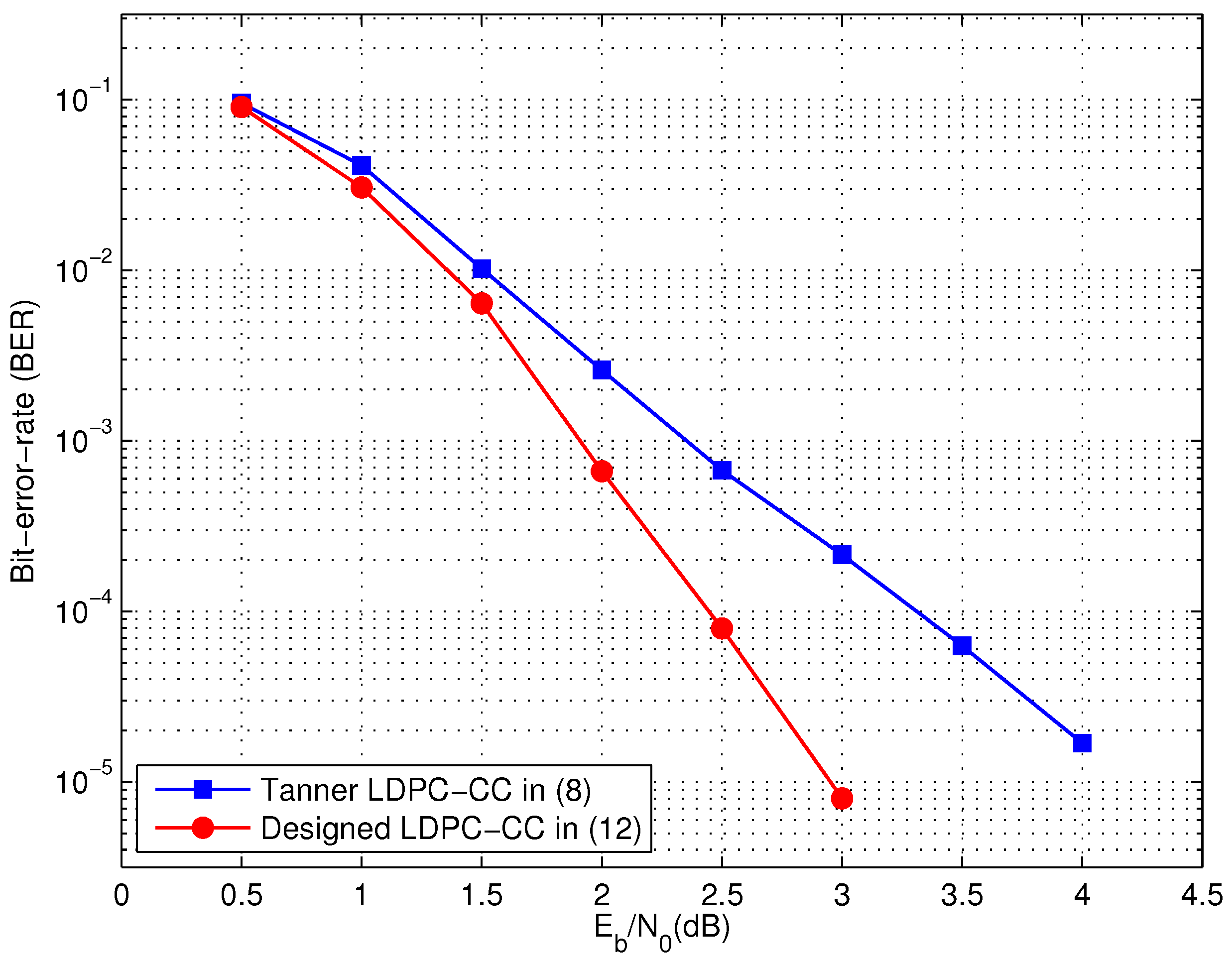
4.2. Improved Distance Spectrum

To delete the non-structured codewords of weight 24 in the (21,3,5) code, we generate a new polynomial syndrome former matrix

$${\mathbf{H}}_{New}^T\left(D\right)={\left[\begin{array}{ccc}1& 1& D^{18}\\ D^{13}& D^{11}& D^{12}\\ D^3& D^{18}& 1\\ D^3& D^4& D^{16}\\ D^{21}& D^{13}& D^{21}\end{array}\right]}_{5\times 3}$$

(12)

where the syndrome former memory $m_s$ is still 21, and both the codes defined in Equations (8) and (12) have girth of 8.

In the case of Equation (12), the super code formed by the second and the third columns contains 10 structured codewords of weight 12. Compared to the super code ${\mathbf{H}}_b^T\left(D\right)$ in Equation (11), the two non-structured codewords ${\mathbf{v}}_b^{11}\left(D\right)$ and ${\mathbf{v}}_b^{12}\left(D\right)$ in Table 3 are eliminated by respectively substituting $D^{11}$, $D^{18}$, and $D^{16}$ for the (2,2)-th, (3,2)-th, and (4,3)-th elements in Equation (11). In addition, similar to the code in Equation (8), arbitrary two columns of Equation (12) representing a super code does not contain any non-structured codewords of weight smaller than 6. As a result, the number of the codewords of weight 24 for the code Equation (12) is reduced to five, and these five codewords are exactly the same as those obtained from Lemma 1.

Applying the distance estimation algorithm in [17] to Equation (12), the number of the codewords of weights 24, 26, 28, 30, and 32 have been reduced from 6, 5, 8, 34, and 53 for the code Equation (8) to 5,0, 0, 0, and 0, respectively. No codewords of weights 26, 28, 30, and 32 are found. The number of low weight codewords has been significantly reduced by carefully choosing the monomials in the polynomial syndrome former matrix. It shows that eliminating the low weight non-structured codewords in the super code improves the distance spectrum of the mother codes.

As shown in Figure 1, the decoding performance of the designed code in Equation (12) is compared to that of the (21, 3, 5) Tanner LDPC-CC in Equation (8). The simulation was carried out assuming binary phase-shift keyed (BPSK) modulation on an additive white Gaussian noise (AWGN) channel with 50 iterations of the on-demand variable node activation [20] sum-product pipeline [4] decoding algorithm for LDPC-CCs. As a benefit of the improved distance spectrum, the bit error ratio (BER) curve of the designed code is consistent lower than that of the Tanner code.

Figure 1. Decoding performance of the codes defined in Equations (12) and (8) .

Figure 1. Decoding performance of the codes defined in Equations (12) and (8) .

4.3. Rules for Designing Practical LDPC-CCs

Through the above analysis, to obtain good distance spectrum when designing practical LDPC-CCs based on a given weight matrix, we propose two design criteria to follow:

• ensuring that each super code does not contain any codewords with weight smaller than the minimum weight of the structured codewords calculated using Lemma 1;
• eliminating the low weight non-structured codewords of the super codes as many as possible.

In order to eliminate the non-structured codewords in the super codes, a two-step calculation is performed as follows:

• Step 1: Compute the enumerator for the structured codewords $E_{\mathcal{C}}$ that the super code contains. In this paper, the structured codewords are calculated based on the formation of the unavoidable cycles [21]. For example, the weight matrix of the super code formed by the second and the third columns of Equation (12) is an all-one matrix of size $5\times 2$. According to the result in [21], this weight matrix contains $\left(\genfrac{}{}{0pt}{}{5}{3}\right)$ = 10 unavoidable cycles of length 12. If an all-one weight matrix contains only two columns or two rows, the structure of an unavoidable cycle of length n in the weight matrix forms a structured codeword of weight $n/2$. Hence, we have $E_{\mathcal{C}}=10$ for the super code formed by arbitrary two columns of Equation (12).
• Step 2: For each entry in the polynomial syndrome former matrix of the super code, we randomly choose a monomial with power smaller than the syndrome former memory $m_s$ and calculate the number of the codewords that the associated super code has. If it is larger than $E_{\mathcal{C}}$, this monomial is replaced by another one until a valid one is found. If all of the monomials with power smaller than $m_s$ have been tested, we simply increase the value of $m_s$ and repeat the process in Step 2.

5. Conclusions

In this paper, the codewords of polynomial-based LDPC-CCs are separated into two categories, i.e., structured codewords and non-structured codewords. In the distance spectrum, the number of the structured codewords is dominated by the size of the polynomial syndrome former matrix ${\mathbf{H}}^T\left(D\right)$, while the number of the non-structured ones depends on the particular monomials or polynomials in ${\mathbf{H}}^T\left(D\right)$. For the design of practical LDPC-CCs, an approach of improving the distance spectrum of the mother code is eliminating the low weight non-structured codewords in the super codes.

References

1. IEEE 802.16e Task Group. IEEE Standard for Local and Metropolitan Area Networks Part 16: Air Interface for Fixed and Mobile Broadband Wireless Access Systems Amendment 2: Physical and Medium Access Control Layers for Combined Fixed and Mobile Operation in Licensed Bands and Corrigendum 1; IEEE Std. 802.16e; IEEE: Piscataway, NJ, USA, 2006. [Google Scholar]
2. European Telecommunications Standards Institute (ETSI). DVB-T2 Implementation Guidelines for a Second Generation Digital Terrestrial Television Broadcasting System (DVB-T2); DVB Blue Book A133 or ETSI TR 102831; ETSI: Sophia Antipolis, France, 2012. [Google Scholar]
3. IEEE 802.11n Task Group. IEEE Draft Standard for Information Technology: Telecommunications and information Exchange Between Systems: Local and Metropolitan Area Networks: Specific Requirements Part 11: Wireless LAN Medium Access Control (MAC) and Physical Layer (PHY) Specifications Amendment 4: Enhancements for Higher Throughput; IEEE Std. 802.11n/D2.00; IEEE: Piscataway, NJ, USA, 2007. [Google Scholar]
4. Felström, A.J.; Zigangirov, K.S. Time-varying periodic convolutional codes with low-density parity-check matrices. IEEE Trans. Inf. Theory 1999, 45, 2181–2191. [Google Scholar] [CrossRef]
5. Lentmaier, M.; Sridharan, A.; Costello, D.J., Jr.; Zigangirov, K.S. Iterative decoding threshold analysis for LDPC convolutional codes. IEEE Trans. Inf. Theory 2010, 56, 5274–5289. [Google Scholar] [CrossRef]
6. Bazzi, L.; Ghazi, B.; Urbanke, R.L. Linear Programming Decoding of Spatially Coupled Codes. IEEE Trans. Inf. Theory 2014, 60, 4677–4698. [Google Scholar] [CrossRef]
7. Schwandter, S.; Graell i Amat, A.; Matz, G. Spatially-coupled LDPC codes for decode-and-forward relaying of two correlated sources over the BEC. IEEE Trans. Commun. 2014, 62, 1324–1337. [Google Scholar] [CrossRef]
8. Abu-Surra, S.; Divsalar, D.; Ryan, W.E. Enumerators for Protograph-Based Ensembles of LDPC and Generalized LDPC Codes. IEEE Trans. Inf. Theory 2011, 57, 858–886. [Google Scholar] [CrossRef]
9. Kasai, K.; Declercq, D.; Poulliat, C.; Sakaniwa, K. Multiplicatively Repeated Nonbinary LDPC Codes. IEEE Trans. Inf. Theory 2011, 57, 6788–6795. [Google Scholar] [CrossRef]
10. Xia, S.; Fu, F. On the minimum pseudocodewords of LDPC codes. IEEE Commun. Lett. 2006, 10, 363–365. [Google Scholar]
11. Chertkov, M.; Stepanov, M. Searching for low weight pseudo-codewords. In Proceedings of the Information Theory and Application Workshop, La Jolla, CA, USA, 29 January–2 February 2007.
12. Smarandache, R.; Pusane, A.E.; Vontobel, P.O.; Costello, D.J., Jr. Pseudocodeword performance analysis for LDPC convolutional codes. IEEE Trans. Inf. Theory 2009, 55, 2577–2598. [Google Scholar] [CrossRef]
13. Bahl, L.R.; Cullum, C.D.; Frazer, W.D.; Jelinek, F. An efficient algorithm for computing free distance. IEEE Trans. Inf. Theory 1972, 18, 437–439. [Google Scholar] [CrossRef]
14. Cedervall, M.; Johannesson, R. A fast algorithm for computing distance spectrum of convolutional codes. IEEE Trans. Inf. Theory 1989, 35, 1146–1159. [Google Scholar] [CrossRef]
15. Rouanne, M.; Costello, D.J., Jr. An algorithm for computing the distance spectrum of trellis codes. IEEE J. Sel. Areas Commun. 1989, 7, 929–940. [Google Scholar] [CrossRef]
16. Bocharova, I.E.; Handlery, M.; Johannesson, R. A BEAST for Prowling in Trees. IEEE Trans. Inf. Theory 2004, 50, 1295–1302. [Google Scholar] [CrossRef]
17. Zhou, H.; Mitchell, D.G.M.; Goertz, N.; Costello, D.J., Jr. Distance spectrum estimation of LDPC convolutional codes. In Proceedings of the 2012 IEEE International Symposium on Information Theory Proceedings (ISIT), Cambridge, MA, USA, 1–6 July 2012.
18. Smarandache, R.; Vontobel, P.O. Quasi-Cyclic LDPC Codes: Influence of proto- and Tanner-graph structure on minimum Hamming distance upper bounds. IEEE Trans. Inf. Theory 2012, 58, 585–607. [Google Scholar] [CrossRef]
19. Tanner, R.M.; Sridhara, D.; Sridharan, A.; Fuja, T.E.; Costello, D.J., Jr. LDPC block and convolutional codes based on circulant matrices. IEEE Trans. Inf. Theory 2004, 50, 2966–2984. [Google Scholar] [CrossRef]
20. Pusane, A.E.; Lentmaier, M.; Zigangirov, K.S.; Costello, D.J., Jr. Reduced complexity decoding strategies for LDPC convolutional codes. In Proceedings of the International Symposium on Information Theory, Chicago, IL, USA, 27 June–2 July 2004.
21. Zhou, H.; Goertz, N. Unavoidable cycles in polynomial-based time-invariant LDPC convolutional codes. In Proceedings of the 11th European Wireless Conference on Sustainable Wireless Technologies, Vienna, Austria, 27–29 April 2011.