Forecasting Monthly Electricity Demands: An Application of Neural Networks Trained by Heuristic Algorithms

Abstract

Electricity demand forecasting plays an important role in capacity planning, scheduling, and the operation of power systems. Reliable and accurate prediction of electricity demands is therefore vital. In this study, artificial neural networks (ANNs) trained by different heuristic algorithms, including Gravitational Search Algorithm (GSA) and Cuckoo Optimization Algorithm (COA), are utilized to estimate monthly electricity demands. The empirical data used in this study are the historical data affecting electricity demand, including rainy time, temperature, humidity, wind speed, etc. The proposed models are applied to Hanoi, Vietnam. Based on the performance indices calculated, the constructed models show high forecasting performances. The obtained results also compare with those of several well-known methods. Our study indicates that the ANN-COA model outperforms the others and provides more accurate forecasting than traditional methods.

1. Introduction

Electric energy plays a fundamental role in business operations all over the world. Our world runs because electricity makes industries, homes, and services work. Therefore, electricity sources must be carefully managed and implemented in order to guarantee the efficient use of electricity. The key to this is to have accurate knowledge of future electricity demands, accurate capacity planning, scheduling, and operations of the power systems. Hence, reliable electricity demand forecasting is needed in order to guarantee that production can meet demand. However, it is difficult to forecast electricity demand because the demand series often contain unpredictable trends, high noise levels, and exogenous variables. Although demand forecasting is difficult to implement, the relevance to forecast the electricity demand has been a much-discussed issue in recent years. This has led to the development of various new tools and methods for forecasting.

Since the accuracy of demand forecasting plays an important role in the success of efficiency planning, energy analysts need guidelines to select the most appropriate forecasting techniques in order to obtain accurate forecasts of electricity consumption trends and to schedule generator planning and maintenance. In general, electricity forecasting demand, accumulated on different time scales, is categorized into short-term, medium-term and long-term demands. The short-term demand forecasting carries out a prediction of the load or energy demand several hours or days ahead. This prediction is very important for the daily operation of facilities. Short-term demand is generally affected by daily life habits, weather conditions, and the temperature. On the other hand, medium-term and long-term demands, which can span periods from a week to a year, are affected by economic and demographic growth, and climate change. Medium-term forecasting provides a prediction of electric demand in the following weeks or months and long-term forecasting predicts the annual power peaks in the following years in order to plan grid extension. Due to the clear interest that medium-term demand forecasting presents in deregulated power systems, in this study, we therefore focus on monthly electric demand forecasting.

Electricity demand forecasting is a complicated task since the demand is affected directly or indirectly by various factors primarily associated with the economy and the climate change. In the past, straight line extrapolations of historical energy consumption trends were adequate methods. However, with the emergence of alternative energies and technologies, fluctuating economic inflation, rapid change in energy prices, industrial development, and global warming issues, the modeling techniques that capture the effect of factors are increasingly necessary, such as average air pressure, average temperature, average wind velocity, rainfall, rainy time, average relative humidity, daylight time, and technological variables. The modelling techniques range from traditional methods, including autoregressive integrated moving average (ARIMA) and multiple linear regression (MLR) (both relying on mathematical approaches), to intelligent techniques, such as fuzzy logic and neural networks [1].

In the early development of forecasting approaches, the most commonly used methods were statistical techniques, such as the trend analysis and extrapolation. It is reasonably easy to apply these kinds of methods due to their simple calculations. Since the total electricity demand includes the demand of factories, enterprises, citizens, and the service industry, forecasting electricity usage requires certain knowledge of past demands in order to take into account the social evolution of future energy demand. Therefore, as past data is needed to forecast future data, a time series analysis of energy demand is usually used to predict future energy use. Time series forecasting is a powerful tool that is widely used to predict time evolution in a number of divergent applications. Different tools, including ARIMA and MLR, have also been developed in the field of time series analysis.

Recently, artificial intelligence techniques have been found to be more effective than traditional methods. Among these, artificial neural networks (ANNs) have been widely applied in various application areas [2,3,4] as well as in the electricity demand forecasting area [5,6,7,8,9,10,11]. ANN is a parallel computing system that uses a large number of connecting artificial neurons. This approach is similar to the function of the biological neural networks. After being trained by historical data, ANNs can be used a prediction tool. Many researchers use ANN to solve electricity demand forecasting problems because of its speed and accuracy. Additionally, ANN can be easily implemented in the development of software. When applying the ANN for forecasting [12,13], most researchers focused on the multi-layer perception (MLP) neural network model. Back-propagation (BP) is the most commonly used training method for training an MLP network. However, many studies have pointed out drawbacks of this algorithm, including the tendency to be trapped in local minima [14] and having a slow convergence [15]. Heuristic algorithms are known for their ability to produce optimal or near optimal solutions for optimization problems. In recent years, several heuristic algorithms—including genetic algorithms (GA) [16], particle swarm optimization (PSO) [17], ant colony optimization (ACO) [18] and differential evolution (DE) [19]—have been proposed for the purpose of training.

Other than these, two heuristic algorithms, the Gravitational Search Algorithm (GSA), and Cuckoo Optimization Algorithm (COA), both inspired by the behavior of natural phenomena, were also developed for solving optimization problems. Through some benchmarking studies, these algorithms have been proven to be powerful and are considered to outperform other algorithms. The GSA, introduced by Rashedi [20], is based on the law of gravity and mass interactions. The comparison of the GSA with other optimization algorithms in some problems shows that the GSA performs well [20,21]. The COA algorithm was developed by Rajabioun [22]. The comparison of the COA with standard versions of PSO and GA also shows that the COA has superiority in fast convergence and near global optimal achievement [22,23]. Moreover, GSA and COA algorithms are efficient optimization algorithms in terms of reducing the aforementioned drawbacks of back propagation. Since these algorithms are relatively new, they have yet to be compared with each other for many different applications.

The merits of the GSA and COA algorithms and the success of ANNs in electricity demand forecasting have encouraged us to use these heuristic algorithms for training ANNs. In this study, several models for electricity demand forecasting have been developed and tested to provide monthly predictions. These models utilize ANNs trained by the three mentioned heuristic algorithms. The error criteria, such as root mean squared error (RMSE) and mean absolute percentage error (MAPE), were used as measures to justify the appropriate model.

The rest of this paper is organized into five sections. After the introduction in Section 1, the literature review is provided in Section 2. The three heuristic algorithms are described in Section 3. Section 4 is dedicated to the research design. The experimental results are discussed in Section 5. Finally, Section 6 gives the conclusions.

2. Literature Review

The ANN has been widely used in different applications. This section provides a glimpse into the literature concerning the use of ANN in electricity demand forecasting. Feilat and Bouzguenda [7] developed a mid-term load forecasting model based on ANN. The proposed model was applied to the Al-Dakhiliya franchise area of the Mazoon Electricity Distribution (MZEC) Company, Oman. The model used monthly load data, temperature, humidity and wind speed from 2006 to 2010 as inputs. The performance indices and the simulation results showed that the forecasting accuracy was satisfactory. The obtained results were also compared with those obtained from the linear regression model. It was found that the ANN-based model outperformed the multiple linear regression method. Kandananond [5] applied different forecasting methods, including ARIMA, ANN, and MLR to forecast electricity demand in Thailand. His study used the historical data of the electricity demand in Thailand from 1986 to 2010. Based on the performance indices, the ANN approach outperformed the ARIMA and MLR methods. Santana et al. [9] used the MLP network with one hidden layer to forecast power consumption in Brazil. The algorithms used in the training of the MLP network were Levenberg–Marquardt and the back propagation. The results showed that the MLP networks presented exceptional results when studying a mid-term forecast. Azadeh et al. [10] used the MLP network to forecast electricity consumption. Monthly electricity consumption in Iran for the past 20 years was collected to train and test the network. The conventional regression model was also applied to the research problem. Through analysis of variance, actual data was compared with forecasting data obtained from the ANN and conventional regression models. It was shown that the ANN approach was superior for estimating the total electricity consumption. Azadeh et al. [11] proposed an artificial neural network (ANN) approach for annual electricity consumption in high energy consumption industrial sectors. Actual data from high energy consuming (intensive) industries in Iran from 1979 to 2003 was used. The ANN forecasting values were compared with actual data and the conventional regression model. The results also indicated that the MLP network can estimate the annual consumption with less error. Deng [24] presents a model based on the multilayer feed-forward neural network to forecast the energy demand for China. The model outperformed the linear regression model in terms of root mean squared error without any over-fitting problem. Hotunluoglu and Karakaya [25] forecasted Turkey’s energy demand by the use of an artificial neural network. Three different scenarios were developed. The obtained energy demand forecasts are useful in future energy planning and policy making process. In [26], the ANN model was tested and compared with other forecasting methods including simple moving average, linear regression, and multivariate adaptive regression splines. It was concluded that the ANN model was effective at forecasting peak building electrical demand in a large government building sixty minutes into the future. Hernández et al. [27] presented a two-stage prediction model based on an ANN to forecast short-term load forecasting of the following day in a microgrid environment. The obtained mean absolute percentage error showed an overall improvement of 52%. Ryu et al. [28] proposed deep neural network-based models to predict the 24-h load pattern day-ahead based on weather, date and past electricity consumptions. The obtained results indicated that the proposed models demonstrated accurate and robust predictions compared to other forecasting models, e.g., mean absolute percentage error and relative root mean square error are reduced by 17% and 22% compared to the shallow neural network model and 9% and 29% compared to the double seasonal Holt–Winters model.

The abovementioned studies revealed that ANN-based models have been successfully used in the area of power electricity forecasting. However, in order to increase the reliability of forecasting results of the ANN-based model, attention is needed to focus on optimizing the parameters of the model. In other words, training phase plays an important role in developing the ANN-based models. In the literature we examined, the BP algorithm, a gradient-based algorithm, has been widely used in the training phase. However, the BP algorithm has some drawbacks. The two recent algorithms, including GSA and COA, are efficient algorithms in terms of reducing the drawbacks of the BP.

Taking into account the available literature, there is still room for improving the ANN-based models for electricity demand forecasting. In this paper, we propose a multilayer feed-forward network improved by the GSA and COA algorithms for forecasting electricity demand. The scientific contributions made by the current research are the new approaches applied herein. Although the models are developed for a specific application, they can be used as basic guides for other application areas.

3. Heuristic Algorithms

In this section, the heuristic algorithms, including GSA and COA used in the training phase are described.

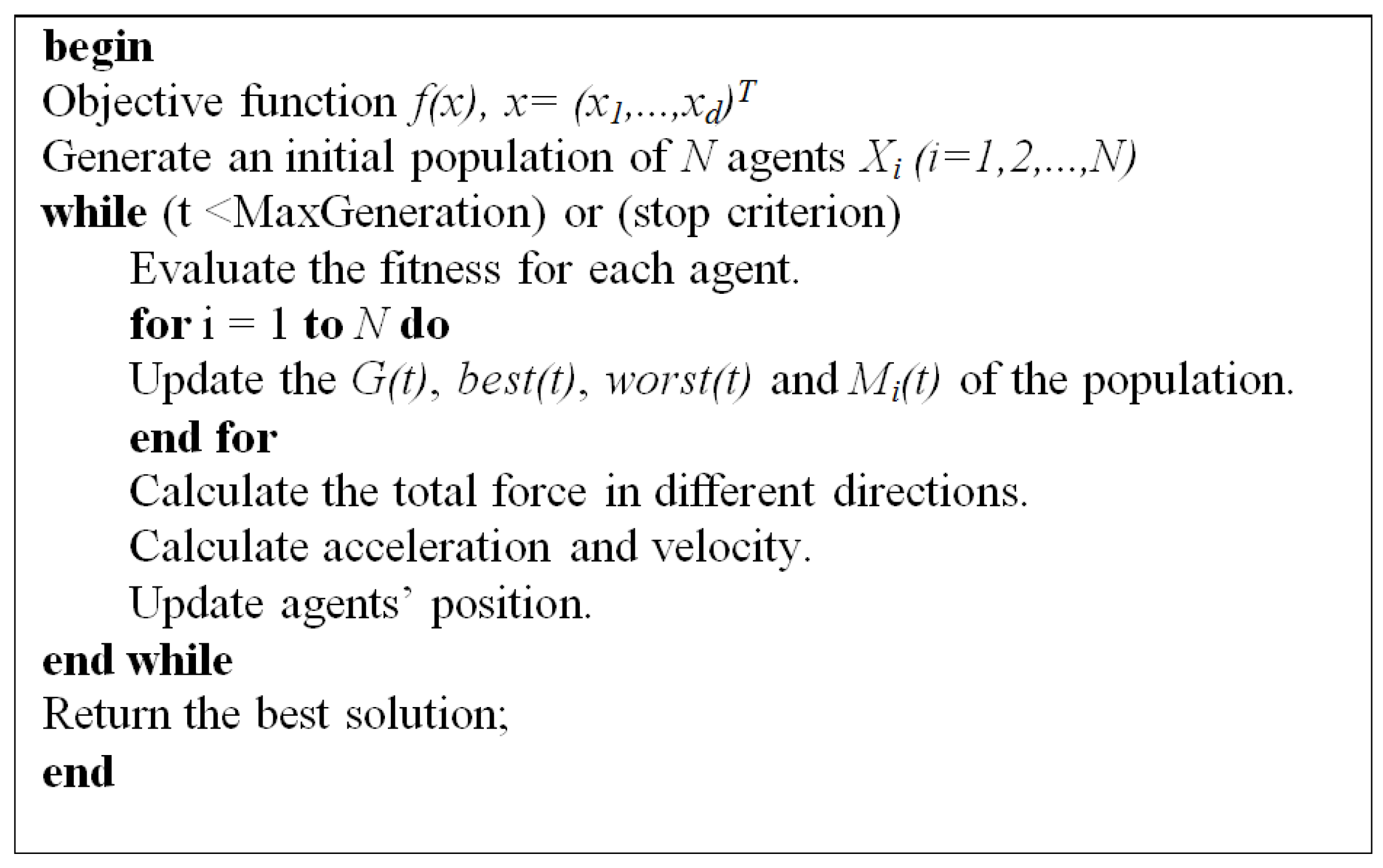
3.1. Gravitational Search Algorithm

The GSA, proposed by Rashedi et al. [20], is based on the physical law of gravity and the law of motion. In the universe, every particle attracts every other particle with a gravitational force that is directly proportional to the product of their masses, and is inversely proportional to the square of the distance between them. The GSA can be considered as a system of agents, called masses, that obey the Newtonian laws of gravitation and masses. All masses attract each other through the gravity forces between them. A heavier mass has a bigger force.

Consider a system with N masses in which the position of the ith mass is defined as follows:

X_i = (x_i¹, ..., x_i^d, ..., x_iⁿ) for i = 1, 2, ..., N,

(1)

where x_i^d is the position of the ith agent in the dth dimension and n presents the dimension of search space. At a specific time, t, the force acting on mass i from mass j is defined as follows:

$$F_{ij}^d(t)=G(t)\frac{M_{pi}(t)\times M_{aj}(t)}{R_{ij}(t)+\epsilon }(x_j^d(t)-x_i^d(t)),$$

(2)

where M_aj denotes the active gravitational mass of agent j; M_pi is the passive gravitational mass of agent i; G(t) represents the gravitational constant at time t; ε is a small constant; and R_ij(t) is the Euclidian distance between agents i and j.

The total force acting on agent i in dimension d is as follows:

$$F_i^d\left(t\right)={\displaystyle \sum _{j=1,j\ne i}^{N}ran{d}_j{F}_{ij}^d\left(t\right)},$$

(3)

where rand_j is a random number in [0, 1]. According to the law of motion, the acceleration of agent i at time t in the dth dimension, a_i^d(t), is calculated as follows:

$$a_i^t(t)=\frac{F_i^d(t)}{M_{ii}(t)},$$

(4)

where M_ii(t) is the mass of object i. The next velocity of an agent is a fraction of its current velocity added to its acceleration. Therefore, the next position and the next velocity can be calculated as:

v_i^d(t + 1) = rand_i × v_i^d(t) + a_i^d(t),

(5)

x_i^d(t + 1) = x_i^d(t) + v_i^d(t + 1).

(6)

The gravitational constant, G, is generated at the beginning and is reduced with time to control the search accuracy. It is a function of the initial value (G₀) and time (t):

G(t) = G(G₀,t).

(7)

Gravitational and inertia masses are calculated by the fitness value. Fitness function is used in each iteration of the algorithm to evaluate the quality of all the proposed solutions to the problem in the current population. The fitness function evaluates how good a single solution in a population is, e.g., suppose that if we find for what x-value a function has its y-minimum, the fitness function for a unit might be the negative y-value (the smaller the value, the higher the fitness function). In general, the fitness value is the objective value of the optimization problem that we want to minimize or maximize. A heavier mass is a more efficient agent. This means that better agents have higher attractions and move more slowly. The gravitational and inertial masses are updated by the following equations:

$$m_i\left(t\right)=\frac{fi{t}_i\left(t\right)-worst\left(t\right)}{best\left(t\right)-worst\left(t\right)},$$

(8)

$$M_i(t)=\frac{m_i(t)}{{\displaystyle \sum _{j=1}^N{m}_j(t)}},$$

(9)

where fit_i(t) denotes the fitness value of agent i at time t, and worst(t) and best(t) represents the weakest and strongest agents in the population, respectively.

For a minimization problem, worst(t) and best(t) are as follows:

$$best(t)=\underset{j\in \left\{1,...,N\right\}}{\min }fi{t}_j(t),$$

(10)

$$worst(t)=\underset{j\in \left\{1,...,N\right\}}{\max }fi{t}_j(t).$$

(11)

For a maximization problem,

$$best(t)=\underset{j\in \left\{1,...,N\right\}}{\max }fi{t}_j(t),$$

(12)

$$worst(t)=\underset{j\in \left\{1,...,N\right\}}{\min }fi{t}_j(t).$$

(13)

The pseudo code of the GSA is given in Figure 1.

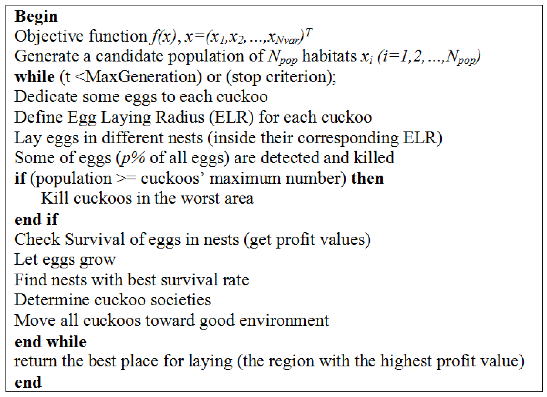
3.2. Cuckoo Optimization Algorithm

Rajabioun [22] developed an algorithm based on the cuckoo’s lifestyle, named the Cuckoo Optimization Algorithm. The lifestyle of the cuckoo species and their characteristics were the basic motivations for the development of this evolutionary optimization algorithm. The cuckoo groups are formed in different areas that are called societies. The cuckoo population in each society consists of two types: mature cuckoos and eggs. The effort to survive among cuckoos constitutes the basis of COA. During the survival competition, some of the cuckoos or their eggs are detected and killed. Then, the survived cuckoo societies try to immigrate to a better environment and start reproducing and laying eggs. Cuckoos’ survival effort hopefully may converge to a place in which there is only one cuckoo society, all having the same survival rates. Therefore, the place in which more eggs survive is the objective that COA wants to optimize. The fast convergence and global optima achievement of this algorithm have been proven through some benchmark problems. The pseudo code of the COA is presented in Figure 2.

In COA, cuckoos lay eggs within a maximum distance from their habitats. This range is called the Egg Laying Radius (ELR). In the algorithm, ELR is defined as:

$$ELR=\alpha \times \frac{Numberofcurrentcuckoo’seggs}{Totalnumberofeggs}\times (va{r}_{hi}-va{r}_{low}),$$

(14)

where $\alpha$ is an integer used to handle the maximum value of ELR, and var_hi and var_low are the upper limit and lower limit of variables in an optimization problem. The society with the best profit value (the highest number of survival eggs) is then selected as the goal point (best habitat) to which other cuckoos should immigrate. In order to recognize which cuckoo belongs to which group, cuckoos are grouped by the K-means clustering method. When moving toward the goal point, each cuckoo only flies λ% of the maximum distance and has a deviation of φ radians. The parameters for each cuckoo are defined as follows:

λ ~ U(0,1),

φ ~ U(−ω, ω),

where λ ~ U(0,1) means that λ is a random number (uniformly distributed) between 0 and 1. ω is a parameter to constrain the deviation from the goal habitat. A ω of π/6 is supposed to be enough for good convergence [22].

4. Research Design

The following subjects were considered in developing theforecasting models.

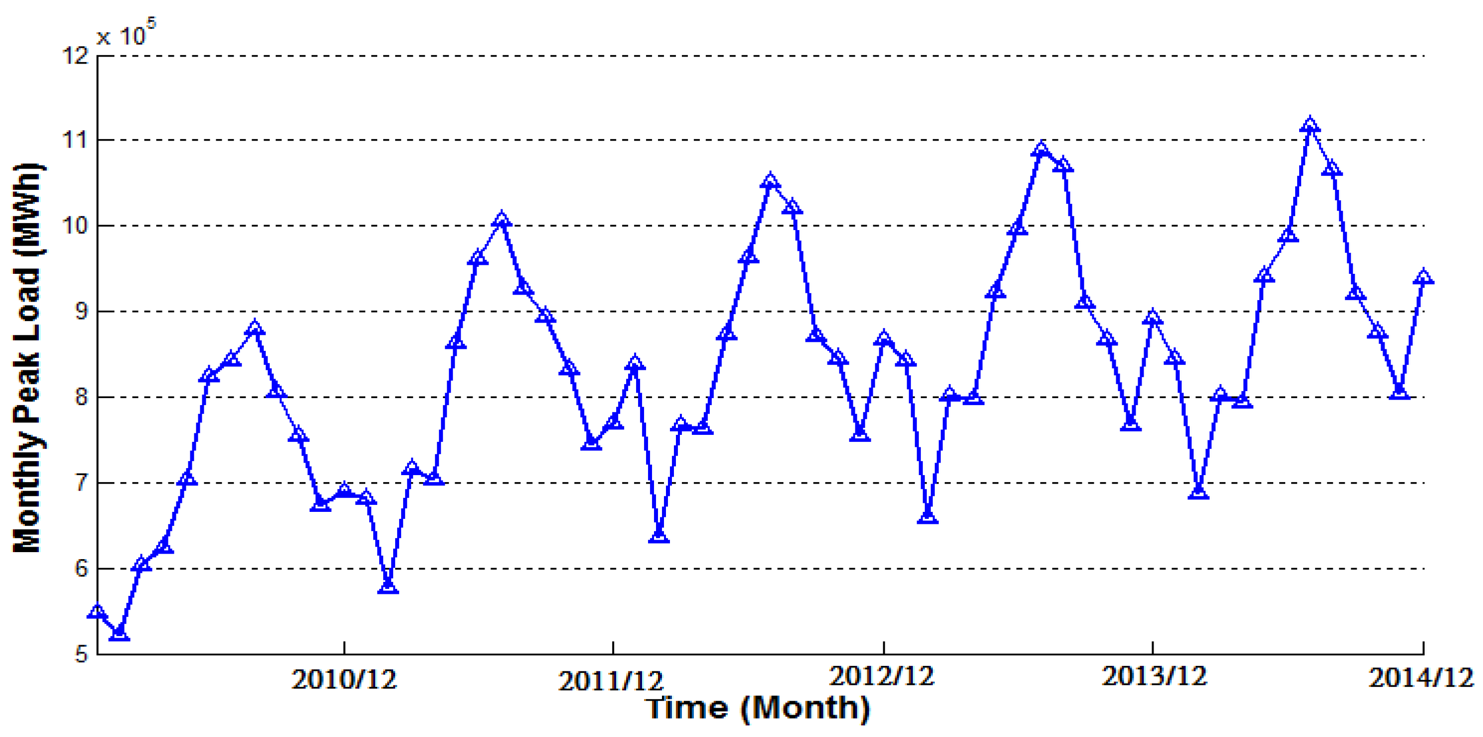
4.1. Historical Data

Due to divergent climate characteristics in northern Vietnam, demand for electricity in Hanoi varies between the summer period (May–August) and the winter period. The demand increases to its full extent during summer and decreases significantly during the rest of the year. Figure 3 shows the monthly demand profile of the Hanoi over the years 2009–2013. The significant increase in electricity demand during the summer period is influenced by the need for operating air conditioners to overcome the high temperatures.

Electricity consumption (MWh) is influenced by several related factors (as shown in

Table 1. Factors used for electricity forecasting.

	Factor
x1	Month index
x2	Average air pressure
x3	Average temperature
x4	Average wind velocity
x5	Rainfall
x6	Rainy time
x7	Average relative humidity
x8	Daylight time

), including month index, average air pressure, average temperature, average wind velocity, rainfall, rainy time, average relative humidity, and daylight time. The historical data regarding these factors were collected from January 2003 to December 2013; in other words, there are 132 monthly data samples. These data were used to determine a forecasting model for future electricity demand. The data used in this study were obtained from the Bureau of Statistics, the National Hydro-Meteorological Service, and the Hanoi Power Company. The available data were divided into two groups. The first group is called the training dataset (84 samples) and includes the data over years 2003–2009 (seven years). The second group is called the testing dataset (48 samples) and includes the data over years 2010–2013 (four years). The training dataset served in model building, while the testing dataset was used for the validation of the developed models.

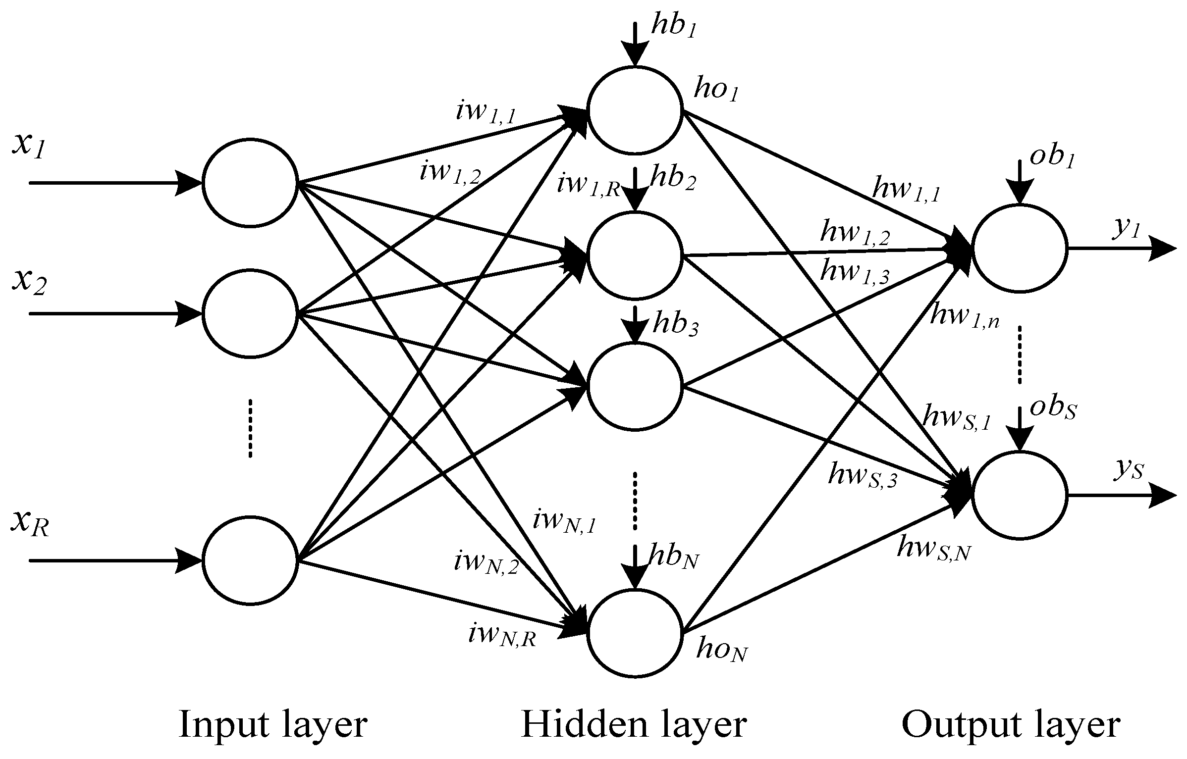
4.2. Structure of the Neural Network

A neural network, in which activations spread only in a forward direction from the input layer through one or more hidden layers to the output layer, is known as a multilayer feed-forward network. For a given set of data, a multi-layer feed-forward network can provide a good nonlinear relationship. Studies have shown that a feed-forward network, even with only one hidden layer, can approximate any continuous function [29]. Therefore, a feed-forward network is an attractive approach [30]. Figure 4 shows an example of a feed-forward network with three layers. In Figure 5, R, N, and S are the numbers of input, hidden neurons, and output, respectively; iw and hw are the input and hidden weights matrices, respectively; hb and ob are the bias vectors of the hidden and output layers, respectively; x is the input vector of the network; ho is the output vector of the hidden layer; and y is the output vector of the network. The neural network in Figure 5 can be expressed through the following equations:

$$h{o}_i=f({\displaystyle \sum _{j=1}^{R}i{w}_{i,j}{x}_j+h{b}_i}),fori=1,...,N,$$

(15)

$$y_i=f({\displaystyle \sum _{k=1}^{N}h{w}_{i,k}h{o}_k+o{b}_i}),fori=1,...,S$$

(16)

where f is an activation function.

When implementing a neural network, it is necessary to determine the structure in terms of the number of layers and the number of neurons in the layers. The larger the number of hidden layers and nodes, the more complex the network is. A network with a structure that is more complicated than necessary may over fit the training data [31]. This means that it may perform well on the data that is included in the training dataset but may perform poorly on the data in a testing dataset.

The structure of an ANN is dictated by the choice of the numbers in the input, hidden, and output layers. Each data set has its own particular structure, and therefore determines the specific ANN structure. The number of neurons comprised in the input layer is equal to the number of features (input variables) in the data. The number of neurons in the output layer is equal to the number of output variables. In this study, the data set includes eight input variables and one output variable; hence, the numbers of neurons in the input and output layers are eight and one, respectively. The three layer feed-forward neural network is utilized in this work since it can be used to approximate any continuous function [32,33]. Regarding the number of hidden neurons, the choice of a proper size of hidden layer has often been studied. However, a rigorous generalized method has not been found [4,34]. Hence, the trial-and-error method is the most commonly used method for estimating the optimum number of neurons in the hidden layer. In this method, various network architectures are tested in order to find the optimum number of hidden neurons [2,3]. In our study, the choice was also made through extensive simulation with different choices for the number of hidden nodes. For each choice, we obtained the performance of the concerned neural networks, and the number of hidden nodes providing the best performance was used for presenting results. The activation function from input to hidden is sigmoid. With no loss of generality, a commonly used form, f(n) = 2/(1 + e⁻²ⁿ) − 1, is utilized, while a linear function is used from the hidden layer to the output layer.

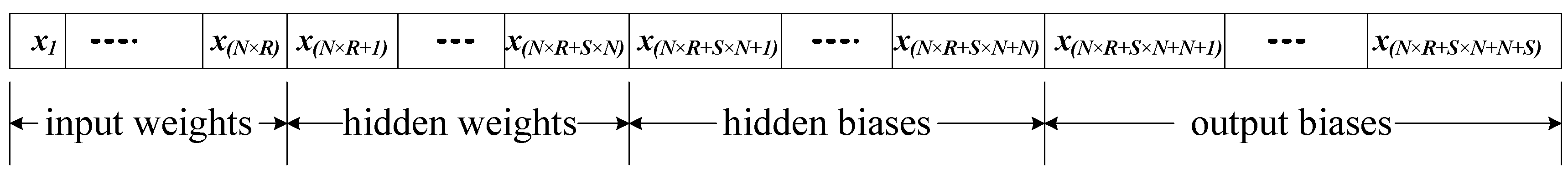
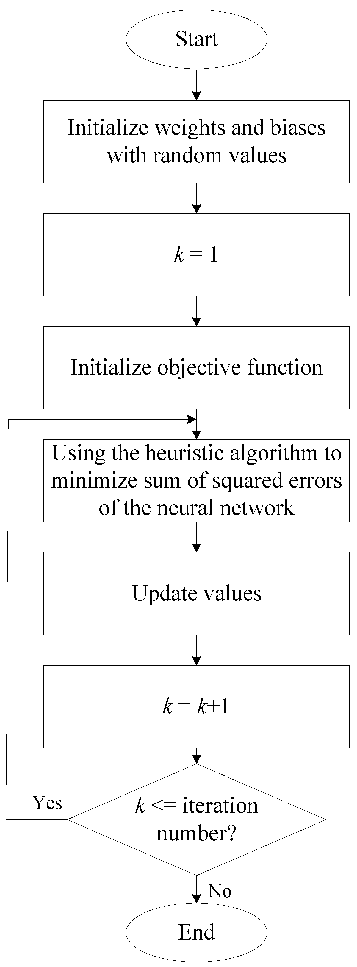
4.3. Training Neural Networks by Heuristic Algorithms

There are three ways of encoding and representing the weights and biases of ANN for every solution in evolutionary algorithms [15]. They are the vector, matrix, and binary encoding methods. In this study, we utilized the vector encoding method and the objective function is to minimize SSE. The two mentioned heuristic algorithms were utilized to search near optimal weights and biases of neural networks. In order to make a comprehensive comparison, the differential evolution (DE) algorithm was also used to train the neural network. We refer to these models hereafter as ANN-GSA, ANN-COA, and ANN-DE. The amount of error is determined by the squared difference between the target output and actual output. In the implementation of the heuristic algorithms to train a neural network, all training parameters, θ = {iw, hw, hb, ob}, are converted into a single vector of real numbers, as shown in Figure 5.

Suppose that there are m input-target sets, the target, t_kp, is the desired output for the given input x_kp for k = 1, 2, …, m and p = 1, 2, ..., S; y_kp and t_kp are forecasting and actual values of pth output unit for sample k. Thus, network variables arranged as iw, hw, hb, and ob are to be changed to minimize an error function, E, such as the SSE (Sum of Squared Errors) between network outputs and desired targets:

$$E={\displaystyle \sum _{k=1}^m{E}_k\mathrm{where}{E}_k={\displaystyle \sum _{p=1}^S{(t_{kp}-y_{kp})}^2}}$$

(17)

Figure 6 describes how heuristic algorithms are being used to train ANN.

4.4. Examining the Performance

To compare the performances of different forecasting models, several criteria are used. These criteria are applied to the trained neural network to determine how well the network works. These criteria are used to compare forecasting values and actual values. They are as follows:

Mean absolute percentage error (MAPE): this index indicates an average of the absolute percentage errors; the lower the MAPE, the better the model is:

$$MAPE=\frac{1}{m}{\displaystyle \sum _{k=1}^m\left|\frac{t_k-y_k}{t_k}\right|},$$

(18)

where t_k is the actual (desired) value, y_k is the forecasting value produced by the model, and m is the total number of observations.

Root mean squared error (RMSE): this index estimates the residual between the actual value and desired value. A model has better performance if it has a smaller RMSE. An RMSE equal to zero represents a perfect fit:

$$RMSE=\sqrt{\frac{1}{m}{\displaystyle \sum _{k=1}^m{\left(t_k-y_k\right)}^2}}.$$

(19)

Mean absolute error (MAE): this index indicates how predicted values are close to the actual values:

$$MAE=\frac{1}{m}{\displaystyle \sum _{k=1}^m\left|t_k-y_k\right|}.$$

(20)

Correlation coefficient (R): this criterion reveals the strength of relationships between actual values and forecasting values. The correlation coefficient has a range from 0 to 1, and a model with a higher R means it has better performance:

$$R=\frac{{\displaystyle \sum _{k=1}^m\left(t_k-\overline{t}\right)\left(y_k-\overline{y}\right)}}{\sqrt{{\displaystyle \sum _{k=1}^m{\left(t_k-\overline{t}\right)}^2{\displaystyle \sum _{k=1}^m{\left(y_k-\overline{y}\right)}^2}}}},$$

(21)

where $\overline{t}=\frac{1}{m}{\displaystyle \sum _{k=1}^m{t}_k}$ and $\overline{y}=\frac{1}{m}{\displaystyle \sum _{k=1}^m{y}_k}$ are the average values of t_k and y_k, respectively.

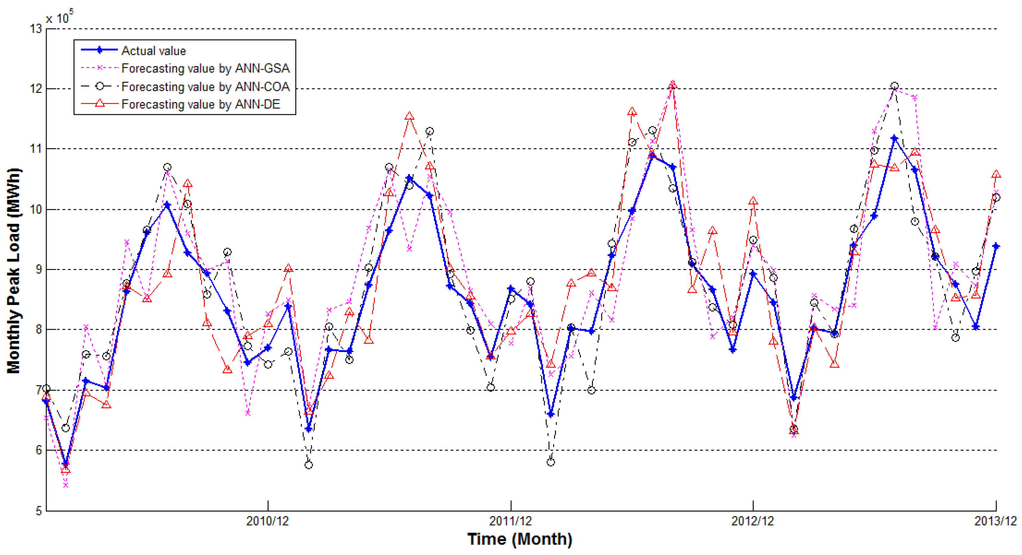
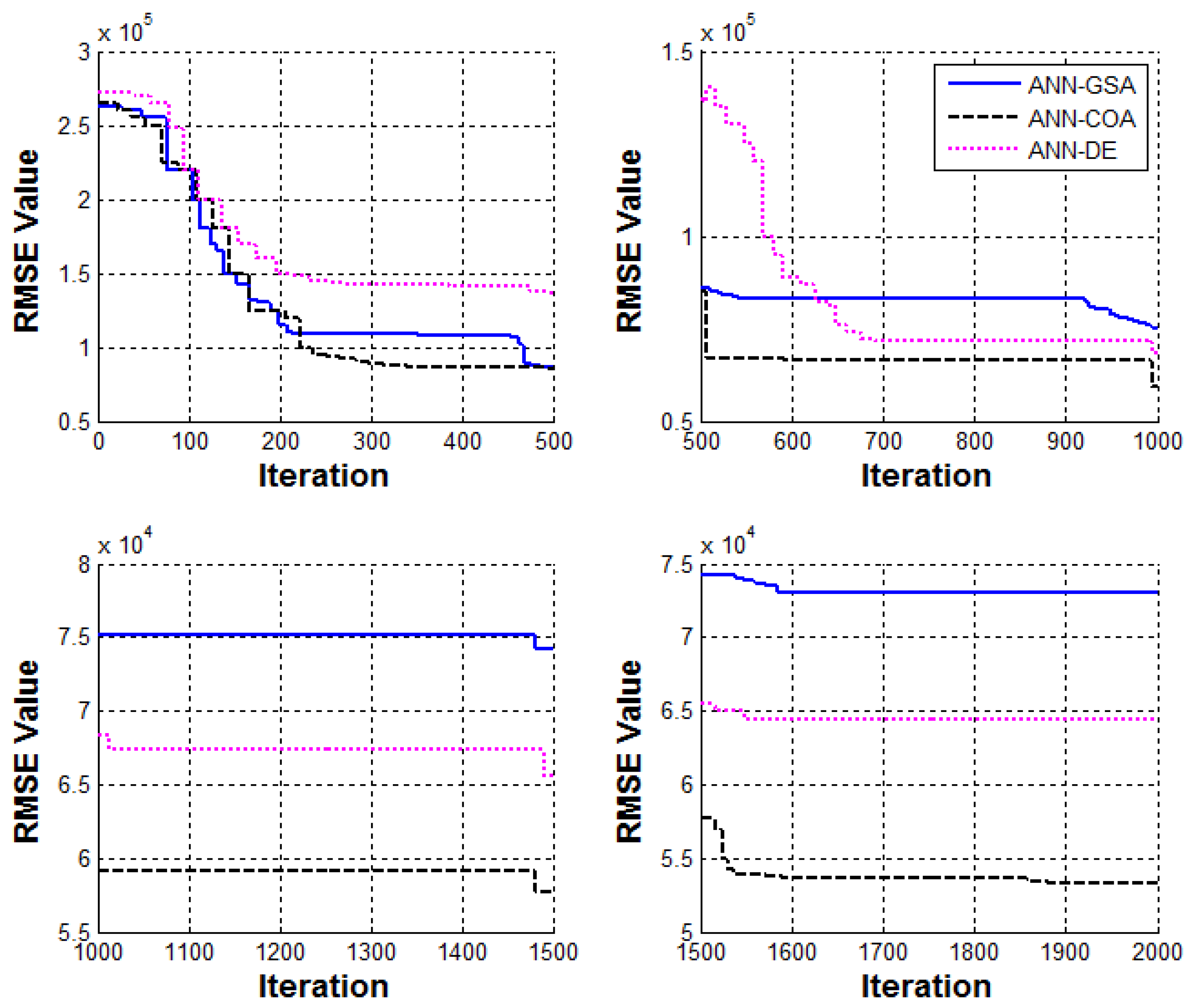
5. Experimental Results and Discussion

The four models were coded and implemented in the Matlab environment (Matlab R2014a, the MathWorks Inc, Natick, MA, USA). As discussed earlier, the one-hidden layer feed-forward neural network architecture was used. The optimum number of neurons in the hidden layer was determined by varying their number, starting with a minimum of one, and then increasing one neuron each time. Hence, various network architectures were tested to achieve the optimum number of hidden neurons. The best performing ANN architecture for the dataset used was then identified, which provided the results with the smallest error values during the training. The best performing architectures for standard ANN, ANN-GSA, ANN-COA, and ANN-DE were found to be 8-6-1, 8-7-1, 8-5-1, and 8-9-1, respectively. A five-fold cross validation method was used to avoid an over-fitting problem. Different parameters of training algorithms were tried to obtain the best performance. For standard ANN, the Back-Propagation (BP) algorithm was used to train the neural networks; the learning and momentum rates were 0.4 and 0.3. For ANN-GSA, the parameters for the GSA algorithm were as follows: the number of initial population was 20 and the gravitational constant in Equation (7) was determined by the function G(t) = G₀ exp(−α × t/T), where G₀ = 100, α = 20, and T was the total number of iterations. For ANN-COA, the parameters were set as follows: the number of initial population was 20 and p% was 10%. For ANN-DE, the crossover rate Cr and the scale factor F were set to 0.9 and 0.85, respectively.

In this study, the number of iterations was chosen as the stopping criterion.

Table 2. Performance statistics of the Artificial Neural Network, Artificial Neural Network trained by Gravitational Search Algorithm (ANN-GSA), Artificial Neural Network trained by Cuckoo Optimization Algorithm (ANN-COA), and Artificial Neural Network trained by Differential Evolution (ANN-DE).

No. of Iterations	Model	MAPE	RMSE	MAE	R
500	ANN	0.1472	137,208	121,152	0.7206
	ANN-GSA	0.0848	86,080	73,540	0.8415
	ANN-COA	0.0843	85,118	73,108	0.8709
	ANN-DE	0.1462	136,819	119,261	0.7608
1000	ANN	0.0826	78,652	120,242	0.7932
	ANN-GSA	0.0764	75,148	66,267	0.8779
	ANN-COA	0.0577	59,073	49,238	0.9287
	ANN-DE	0.0671	68,325	56,409	0.9332
1500	ANN	0.0803	75,524	93,142	0.7988
	ANN-GSA	0.0759	74,218	63,733	0.8842
	ANN-COA	0.0578	57,731	49,100	0.9372
	ANN-DE	0.0633	65,529	56, 937	0.9382
2000	ANN	0.0796	73,482	76,249	0.8020
	ANN-GSA	0.0731	72,980	64,267	0.8892
	ANN-COA	0.0478	53,308	48,238	0.9386
	ANN-DE	0.0582	64,372	55,021	0.8921

gives the performance statistics on the test dataset for the ANN, ANN-GSA, ANN-COA, and ANN-DE at the 500th iteration and 1000th iteration. As can be seen from Table 2, the ANN-COA has smaller MAPE, RMSE, and MAE values as well as a bigger R value than those of the ANN, ANN-GSA and ANN-DE. This means that the ANN-COA had a better overall performance in forecasting. At the 1000th iteration, the performance statistics MAPE, RMSE, MAE, and R obtained by the ANN-COA model were calculated as 0.0577, 59,073, 49,238, and 0.9287, respectively. These results were highly correlated. At the 500th iteration, the ANN-GSA had a better performance than the ANN-DE. However, at the 1000th iteration, the ANN-CS outperformed the ANN-GSA. Figure 8 presents the time series of actual and forecasting values obtained using the three models. The trends in the plots of the time series suggest that the ANN-based models are appropriate for electricity demand forecasting. It can also be concluded that the standard ANN model had the worst performance due to the fact that the BP algorithm (a gradient-based algorithm) has the tendency to become trapped in local minima. Therefore, hereafter, the performance statistics of ANN are excluded in Figure 7 and Figure 8.

Figure 8 depicts the RMSE values obtained in the training phase for the three models in 1000 iterations. At the 2000th iteration, the RMSE values of the ANN, ANN-GSA, ANN-COA, and ANN-DE were 73,482, 72,980, 53,308, and 64,358, respectively. The ANN-COA and ANN-GSA had a faster convergence than the ANN-DE. The ANN-GSA was trapped in local minima of the parameter space; therefore, it yielded poor performance. Among the three models, the ANN-COA has the capability of avoiding premature convergence and exploring the whole search space.

In order to evaluate the performance of the ANN-based models, the ARIMA and MLR methods were also applied to the problem. The details of these methods can be found in the relevant literature, which is beyond the scope of this work. After a few testing attempts, the ARIMA model was selected as ARIMA (2,1,1). These models were also implemented in Matlab R2014a. The results obtained by these models were recorded and are shown in

Table 3. Performance statistics of the Autoregressive Integrated Moving Average (ARIMA) and Multiple Linear Regression (MLR).

Method	MAPE	RMSE	MAE	R
MLR	0.1662	170,540	145,910	0.6031
ARIMA (2,1,1)	0.1603	152,070	136,260	0.7043

. As can be seen from Table 3, the ARIMA had a better performance than the MLR. However, when compared with the results from Table 2, the ANN-based models surpassed the ARIMA and MLR. Based on the results presented in this section, it can be inferred that the ANN-based models perform better than traditional forecasting methods (ARIMA and MLR) and the ANN-COA model is clearly superior to its counterparts. Regarding the complexity of the models, the ARIMA model requires less computational time than the other models. ANN-based models are more complex, involving a network of processing elements.

6. Conclusions

Understanding electricity demand is a critical factor that is required for ensuring future stability and security. Executives and government authorities need this information for decision making in energy markets. In this study, a new approach based on ANNs and heuristic algorithms for electricity demand forecasting is proposed. The proposed approach and other well known forecasting methods, ARIMA and MLR, were used to forecast the electricity demand in Hanoi, Vietnam based on historical data from 2003 to 2013. The results indicate that the ANN-COA is the best model to fit the historical data. This study using the neural networks as a modelling tool for forecasting electricity demand has shown the benefits of the application of neural networks. Therefore, this work has made a contribution to the development of forecasting methods. Further studies may include different segments of electricity consumption, including residential, industrial, agricultural, government commerce, and city services. Province based forecasting is also essential for distribution companies. Technical loss should be taken into account when analyzing electricity demand because this parameter may have a tremendous impact.

References

1. Suganthia, L.; Samuelb, A.A. Energy models for demand forecasting—A review. Renew. Sustain. Energy Rev. 2012, 16, 1223–1240. [Google Scholar] [CrossRef]
2. Dogan, E.; Akgungor, A. Forecasting highway casualties under the effect of railway development policy in Turkey using artificial neural networks. Neural Comput. Appl. 2013, 22, 869–877. [Google Scholar] [CrossRef]
3. Erzin, Y.; Oktay Gul, T. The use of neural networks for the prediction of the settlement of one-way footings on cohesionless soils based on standard penetration test. Neural Comput. Appl. 2014, 24, 891–900. [Google Scholar] [CrossRef]
4. Bhattacharya, U.; Chaudhuri, B. Handwritten Numeral Databases of Indian Scripts and Multistage Recognition of Mixed Numerals. IEEE Trans. Pattern Anal. Mach. Intell. 2009, 31, 444–457. [Google Scholar] [CrossRef] [PubMed]
5. Kandananond, K. Forecasting Electricity Demand in Thailand with an Artificial Neural Network Approach. Energies 2011, 4, 1246–1257. [Google Scholar] [CrossRef]
6. Chang, P.C.; Fan, C.Y.; Lin, J.J. Monthly electricity demand forecasting based on a weighted evolving fuzzy neural network approach. Int. J. Electr. Power Energy Syst. 2011, 33, 17–27. [Google Scholar] [CrossRef]
7. Feilat, E.A.; Bouzguenda, M. Medium-term load forecasting using neural network approach. In Proceedings of the IEEE PES Conference on Innovative Smart Grid Technologies—Middle East (ISGT Middle East), Jeddah, Saudi Arabia, 17–20 December 2011; pp. 1–5.
8. Amjady, N.; Keynia, F. A New Neural Network Approach to Short Term Load Forecasting of Electrical Power Systems. Energies 2011, 4, 488–503. [Google Scholar] [CrossRef]
9. Santana, Á.L.; Conde, G.B.; Rego, L.P.; Rocha, C.A.; Cardoso, D.L.; Costa, J.C.W.; Bezerra, U.H.; Francês, C.R.L. PREDICT—Decision support system for load forecasting and inference: A new undertaking for Brazilian power suppliers. Int. J. Electr. Power Energy Syst. 2012, 38, 33–45. [Google Scholar] [CrossRef]
10. Azadeh, A.; Ghaderi, S.F.; Sohrabkhani, S. Forecasting electrical consumption by integration of Neural Network, time series and ANOVA. Appl. Math. Comput. 2007, 186, 1753–1761. [Google Scholar] [CrossRef]
11. Azadeh, A.; Ghaderi, S.F.; Sohrabkhani, S. Annual electricity consumption forecasting by neural network in high energy consuming industrial sectors. Energy Convers. Manag. 2008, 49, 2272–2278. [Google Scholar] [CrossRef]
12. Vahidinasab, V.; Jadid, S.; Kazemi, A. Day-ahead price forecasting in restructured power systems using artificial neural networks. Electr. Power Syst. Res. 2008, 78, 1332–1342. [Google Scholar] [CrossRef]
13. Bashir, Z.A.; El-Hawary, M.E. Applying wavelets to short-term load forecasting using PSO-based neural networks. IEEE Trans. Power Syst. 2009, 24, 20–27. [Google Scholar] [CrossRef]
14. Gori, M.; Tesi, A. On the problem of local minima in back-propagation. IEEE Trans. Pattern Anal. Mach. Intell. 1992, 14, 76–86. [Google Scholar] [CrossRef]
15. Zhang, J.R.; Zhang, J.; Lock, T.; Lyu, M. A hybrid particle swarm optimization–back-propagation algorithm for feed-forward neural network training. Appl. Math. Comput. 2007, 185, 1026–1037. [Google Scholar]
16. Goldberg, D.E. Genetic Algorithms in Search, Optimization and Machine Learning; Addison Wesley: Boston, MA, USA, 1989. [Google Scholar]
17. Kennedy, J.; Eberhart, R.C. Particle swarm optimization. In Proceedings of the IEEE International Conference on Neural Networks, Perth, Australia, 1995; Volume 4, pp. 1942–1948.
18. Dorigo, M.; Maniezzo, V.; Golomi, A. Ant system: Optimization by a colony of cooperating agents. IEEE Trans. Syst. Man Cybern. 1996, 26, 29–41. [Google Scholar] [CrossRef] [PubMed]
19. Storn, R.; Price, K.V. Differential evolution—A simple and efficient heuristic for global optimization over continuous Spaces. J. Glob. Optim. 1997, 11, 341–359. [Google Scholar] [CrossRef]
20. Rashedi, E.; Nezamabadi-Pour, H.; Saryazdi, S. GSA: A Gravitational Search Algorithm. Inf. Sci. 2009, 179, 2232–2248. [Google Scholar] [CrossRef]
21. Duman, S.; Güvenç, U.; Yörükeren, N. Gravitational Search Algorithm for Economic Dispatch with Valve-Point Effects. Int. Rev. Electr. Eng. 2010, 5, 2890–2895. [Google Scholar]
22. Rajabioun, R. Cuckoo optimization algorithm. Appl. Soft Comput. 2011, 11, 5508–5518. [Google Scholar] [CrossRef]
23. Balochian, S.; Ebrahimi, E. Parameter Optimization via Cuckoo Optimization Algorithm of Fuzzy Controller for Liquid Level Control. J. Eng. 2013, 2013, 1–7. [Google Scholar] [CrossRef]
24. Deng, J. Energy Demand Estimation of China Using Artificial Neural Network. In Proceedings of the 2010 Third International Conference on Business Intelligence and Financial Engineering, Hong Kong, China, 13–15 August 2010; pp. 32–34.
25. Hotunluoglu, H.; Karakaya, E. Forecasting Turkey’s Energy Demand Using Artificial Neural Networks: Three Scenario Applications. Ege Acad. Rev. 2011, 11, 87–94. [Google Scholar]
26. Grant, J.; Eltoukhy, M.; Asfour, S. Short-Term Electrical Peak Demand Forecasting in a Large Government Building Using Artificial Neural Networks. Energies 2014, 7, 1935–1953. [Google Scholar] [CrossRef]
27. Hernández, L.; Baladrón, C.; Aguiar, J.M.; Calavia, L.; Carro, B.; Sánchez-Esguevillas, A.; Sanjuán, J.; González, Á.; Lloret, J. Improved Short-Term Load Forecasting Based on Two-Stage Predictions with Artificial Neural Networks in a Microgrid Environment. Energies 2013, 6, 4489–4507. [Google Scholar] [CrossRef]
28. Ryu, S.; Noh, J.; Kim, H. Deep Neural Network Based Demand Side Short Term Load Forecasting. Energies 2017, 10, 3. [Google Scholar] [CrossRef]
29. Funahashi, K. On the approximate realization of continuous mappings by neural networks. Neural Netw. 1989, 2, 183–192. [Google Scholar] [CrossRef]
30. Norgaard, M.; Poulsen, N.; Hansen, L. Neural Networks for Modeling and Control of Dynamic Systems. A Practitioner’s Handbook; Springer: London, UK, 2000. [Google Scholar]
31. Caruana, R.; Lawrence, S.; Giles, C. Overfitting in neural networks: Backpropagation, conjugate gradient, and early stopping. Available online: https://papers.nips.cc/paper/1895-overfitting-in-neural-nets-backpropagation-conjugate-gradient-and-early-stopping.pdf (accessed on 8 March 2017).
32. Cybenko, G. Approximation by superposition of a sigmoid function. Math. Control Signals Syst. 1989, 2, 303–314. [Google Scholar] [CrossRef]
33. Hornik, K.; Stinchombe, M.; White, H. Universal Approximation of an unknown Mapping and its Derivatives Using Multilayer Feed forward Networks. Neural Netw. 1990, 3, 551–560. [Google Scholar] [CrossRef]
34. Alallayah, K.; Amin, M.; AbdElwahed, W.; Alhamami, A. Applying Neural Networks for Simplified Data Encryption Standard (SDES) Cipher System Cryptanalysis. Int. Arab J. Inf. Technol. 2012, 9, 163–169. [Google Scholar]
Figure 1. Pseudo code of the Gravitational Search Algorithm (GSA).
Information 08 00031 g001
Figure 2. Pseudo code of the Cuckoo Optimization Algorithm (COA).
Information 08 00031 g002
Figure 3. The load time series from January 2009 to December 2013.
Information 08 00031 g003
Figure 4. A feed-forward network with three layers.
Information 08 00031 g004
Figure 5. The vector of training parameters.
Information 08 00031 g005
Figure 6. Using heuristic algorithm to train neural networks.
Information 08 00031 g006
Figure 7. The forecasting performance of Artificial Neural Network trained by Gravitational Search Algorithm (ANN-GSA), Artificial Neural Network trained by Cuckoo Optimization Algorithm (ANN-COA), and Artificial Neural Network trained by Differential Evolution (ANN-DE).
Information 08 00031 g007
Figure 8. Root mean squared error (RMSE) values in 2000 iterations.
Information 08 00031 g008