Data-Aided and Non-Data-Aided SNR Estimators for CPM Signals in Ka-Band Satellite Communications

Abstract

Adaptive coded and modulation (ACM) is an effective measure to resist rain attenuation in Ka-band satellite communications. The accuracy of the estimator for signal-to-noise ratio (SNR) is one of the main factors that affect ACM performance. This paper establishes the channel model of satellite communication in Ka-band and derives and analyzes data-aided (DA) maximum likelihood (ML) and method-of-moments estimators for SNR of continuous phase modulation (CPM) in Ka-band fading channel. Simulations and analysis indicate that the normalized mean square error (NMSE) of the DA ML estimator is closer to the Cramer-Rao bounds (CRB) at low SNR, but the performance worsens with the SNR increases from medium to high values. The M₂M₄ estimator performs poorly at low SNR and best at medium SNR. When the SNR is low, the performance of the DA ML estimator is better than the M₂M₄ estimator; however, the two estimators have similar performance when SNR is high. The performances of the two estimators will become increasingly better the greater the lengths of the observation signals become. However, the influence of the signal length will become increasingly smaller as the SNR becomes larger.

1. Introduction

Many bands can be used for satellite communication; these bands include L, S, C, Ku, and Ka bands. Adopting a high-frequency band in the construction of a broadband satellite communication network is necessary to address the issue of the limited bandwidth of satellite communication. Current high-throughput satellite (HTS) systems for broadband-distributed user access are designed following two main concepts: The use of Ka-band radio frequency (RF) links both for the forward and for the return link; The use of multispot coverage: this technique is largely applied to increase the system throughput through frequency reuse and system reconfigurability [1]. While with the exploitation of extremely high-frequency (EHF) bands (30–300 GHz) for broadband transmission over satellite links, the Q-V band (30–50 GHz) and W-band (75–110 GHz) seem to offer very promising perspectives [2]. This paper use Ka-band as the operating frequency band for satellite communication because of the advantages of the wideband, little disturbance, and small-sized terminals [3].

At frequencies beyond 10 GHz, rainfall is one of the important atmospheric parameters (hydrometeors) which causes signal degradation along both terrestrial and satellite tracks [4,5,6]. Therefor the rain attenuation is considered to be the main factor in Ka-band satellite communications [7,8,9]. Rain rate data was measured through OTT Parsivel, which shows the rain rate of about 50 mm/h and attenuation of 10.7, 11.6, and 11.3 dB for 12.25, 19.8, and 20.73 GHz, respectively, for 0.01% of the time for the combined values of rain rate and rain attenuation statistics [10,11]. The design of millimeter wave communication links and the study of propagation impairments at higher frequencies due to a hydrometeor, particularly rain, require the knowledge of 1-min. rainfall rate data [12,13]. ITU-R series play an important role in prediction of rainfall attenuation. The effectiveness of ITU-RP.618-12 method is seen in which the better prediction for rain-induced attenuation and the propagation data and prediction methods required for the design of Earth-space telecommunication systems. ITU-RP.311-16 shows the data acquisition, representation and analysis of radio wave propagation studies [14]. The adaptive-coded and modulation (ACM) system is an effective measure to resist rain attenuation because it can guarantee communication quality and overcome the problem of system resource waste caused by rainfall reserve. Hence, ACM could be one of the technologies with the most potential and value.

The basic principle of ACM technology in Ka-band satellite communication is to estimate the signal-to-noise ratio (SNR) at the receiver and feed the value back to the transmitter. The transmitter changes the coding and modulation mode according to the signal-to-noise ratio (SNR). The common modulation used for satellite communications mainly includes multiple phase shift keying (M-PSK) and Multiple Quadrature Amplitude Modulation (M-QAM) [15]. The limitations of these modulation techniques in the frequency band utilization restrict the development of satellite communications because of the continuous improvement of the channel bandwidth requirements of satellite communications. Continuous phase modulation (CPM) is a constant envelope continuous phase modulation signal with a wide bandwidth, high power utilization, and a certain coding gain compared with phase shift keying (PSK) modulation [16,17]. CPM also has a larger signal state under some specific parameters, which makes a larger matched filters, leading to a high implementation complexity of optimal receiver. However, this problem can be solved with the effective choice of parameters and the use of large capacity devices. Hence, CPM has become one of the most important modulation methods in recent years. This paper uses the CPM signal to replace the PSK modulation as the main modulation mode of ACM system in Ka-band satellite communication.

The accuracy of channel state estimation is one of the main factors that affect the performance of ACM, and the SNR is used to characterize channel state information. The SNR estimation method consists of time domain and frequency domain methods. The time domain method can be divided into data-aided (DA) and non-data aided (NDA) methods [18]. The DA method has higher estimation accuracy than NDA method but involves the insertion of a periodic pilot sequence, which is inefficient. A significant number of studies have been conducted on SNR estimation technology in recent years. The DA and NDA ML SNR estimators for CPM signals were studied by Rice, and the effects of the frequency and phase shifts were also considered. However, the simulation is based on the additive Gaussian white noise (AWGN) channel [19]. Chang studied the SNR estimation method for MPSK signals in Nakagami fading channels and proposed a joint estimation algorithm for SNR and fading factor; however, the algorithm is suitable only for MPSK [20]. Based on the second generation digital satellite TV broadcasting standard (DVB-S2), Wu proposed an SNR estimation algorithm based on eigenvalue decomposition in the AWGN channel; however, it is not used in the Ka band [21]. Li proposed the ML SNR estimation algorithm for M-APSK signals in slow time-varying fading channels, which improve the estimation accuracy under low SNR, but the CPM signal is not introduced [22].

The SNR estimation algorithm in Ka-band satellite communication is based mostly on PSK modulation, and no relevant literature applies the CPM signal to the ACM technology in Ka-band satellite communication. This study analyzes the channel model in Ka-band satellite communication and focuses on studies on SNR estimation algorithm for CPM signals in the Ka-band fading channel. DA ML and M₂M₄ estimators are derived and analyzed. The SNR fitting curve, normalized mean square error (NMSE), and CRLB are used to analyze the performance of the estimation algorithm, and the effects of several parameters on SNR estimation are discussed.

The paper is organized as follows. Section 2 establishes the channel model of Ka-band satellite communications. Section 3 presents the schematic of the system and the expression of the received signal. Section 4 develops and analyzes two SNR estimators and provides the expression of CRLB. Section 5 presents the simulation results. Section 6 gives the conclusions.

2. Channel Model of Ka-Band Satellite Communication

2.1. Attenuation Factor

Many factors in the atmosphere cause the additional decline of the signal in the Ka-band satellite communication, precipitation, water vapor, clouds, oxygen, and flickers. The most important factor is rain attenuation, which is related to frequency, weather conditions, and system availability. These factors can be considered in the satellite communication link by modifying the free space propagation formula.

Signal fading caused by rainfall is the most serious propagation loss in Ka-band satellite communication. Measured data show that rain attenuation is a function of carrier frequency and system feasibility. In the case of large elevation [22], $L_r$ can be expressed as

$$L_r=C_1\exp ({\delta }_{1}f)+C_2\exp ({\delta }_{2}f)-(C_1+C_2)(\text{dB})$$

(1)

where $C_1$, $C_2$, ${\delta }_1$, and ${\delta }_2$ are the functions of the system availability, and $f$ is the carrier frequency. When the elevation is small, the formula can be simplified as

$$L_r(\theta )=L_r({\theta }_0)\sin \theta /\sin {\theta }_0(\text{dB}),$$

(2)

where $\theta$ is the elevation of the earth station, and ${\theta }_0$ is the reference elevation.

Atmospheric absorption includes mainly oxygen and water vapor absorption. The International Telecommunication Union Radio communications sector (ITU-R) provides the expression of oxygen absorption loss under a slant path as follows

$$L_{\mathrm{o}}=\frac{h_o{\gamma }_o}{\sin \theta }(\text{dB}),$$

(3)

where $h_o$ is the effective height of dry air, ${\gamma }_o$ is the oxygen loss coefficient, and $\theta$ is the elevation. ITU-R also gives the expression of water vapor absorption loss

$$L_w=\frac{h_w{\gamma }_w}{\sin \theta }(\text{dB}),$$

(4)

where $h_w$ is the effective height of water vapor, ${\gamma }_w$ is the water vapor loss coefficient, and $\theta$ is the elevation.

The size of cloud attenuation is related to the content and temperature of liquid water. ITU-R gives the expression of cloud attenuation

$$L_{\mathrm{c}}=\frac{0.4095h}{i(1+{(\frac{2+r}{i})}^2)\sin \theta }(\text{dB})$$

(5)

where $h$ refers to the cloud layer thickness, $r$ and $i$ are the real and imaginary parts of the dielectric constant of water, respectively, and $\theta$ is the elevation.

The refractive index of the propagation path rises randomly with position and time. A flicker exhibits rapid fluctuation when the radio waves pass through the atmosphere, causing fast fluctuation of the amplitude and phase of the radio wave. A flicker can attenuate and enhance the electric wave signal.

ITU-R suggests that the total attenuation value $L_t$ can be expressed as

$$L_t=L_{\mathrm{o}}+L_w+L_c+\sqrt{{L_r}^2+{L_s}^2}(\text{dB}).$$

(6)

The free space propagation formula in the design of the Ka-band satellite communication system should be amended with the additional attenuation caused by rainfall, atmosphere, cloud, and flicker. It can be expressed as

$$P_R=(P_T{A}_T{A}_R/c^2{l}^2)\cdot (f^2/L_t)=(P_T{A}_T{A}_R/c^2{l}^2)\cdot m(f,p)(w),$$

(7)

where $P_R$ and $P_T$ are the average power of the receiver and transmitter, respectively, $(w)$ is the unit, $f$ is the carrier frequency, $l$ is the distance from satellite to earth terminal, $c$ is the speed of light in vacuum, $A_R$ and $A_T$ are the effective contact areas of receiving antenna and transmitting antenna, respectively, $L_t$ is the total attenuation for link, and $p$ refers to system unavailability.

Formula (7) shows that the multiplicative factor $m(f,p)=f^2/L_t$ increases with the increase of $f$. $L_t$ increases rapidly with the increase of $f$ and the feasibility of the system. $m(f,p)$ decreases with the increase of $f$. Numerical calculations show that the multiplicative factor $m(f,p)$ remains unchanged in a wide frequency range when system feasibility is low (e.g., the system feasibility is less than 99.7%) [23]. The total fading of the channel can be considered as non-frequency selective fading given that the feasibility of the Ka-band satellite communication system is usually less than 99.7%. The entire channel can be viewed as flat fading and AWGN; flat fading is slow over time and is related only to the weather [24].

2.2. Statistical Channel Model of Ka-Band Satellite Communication

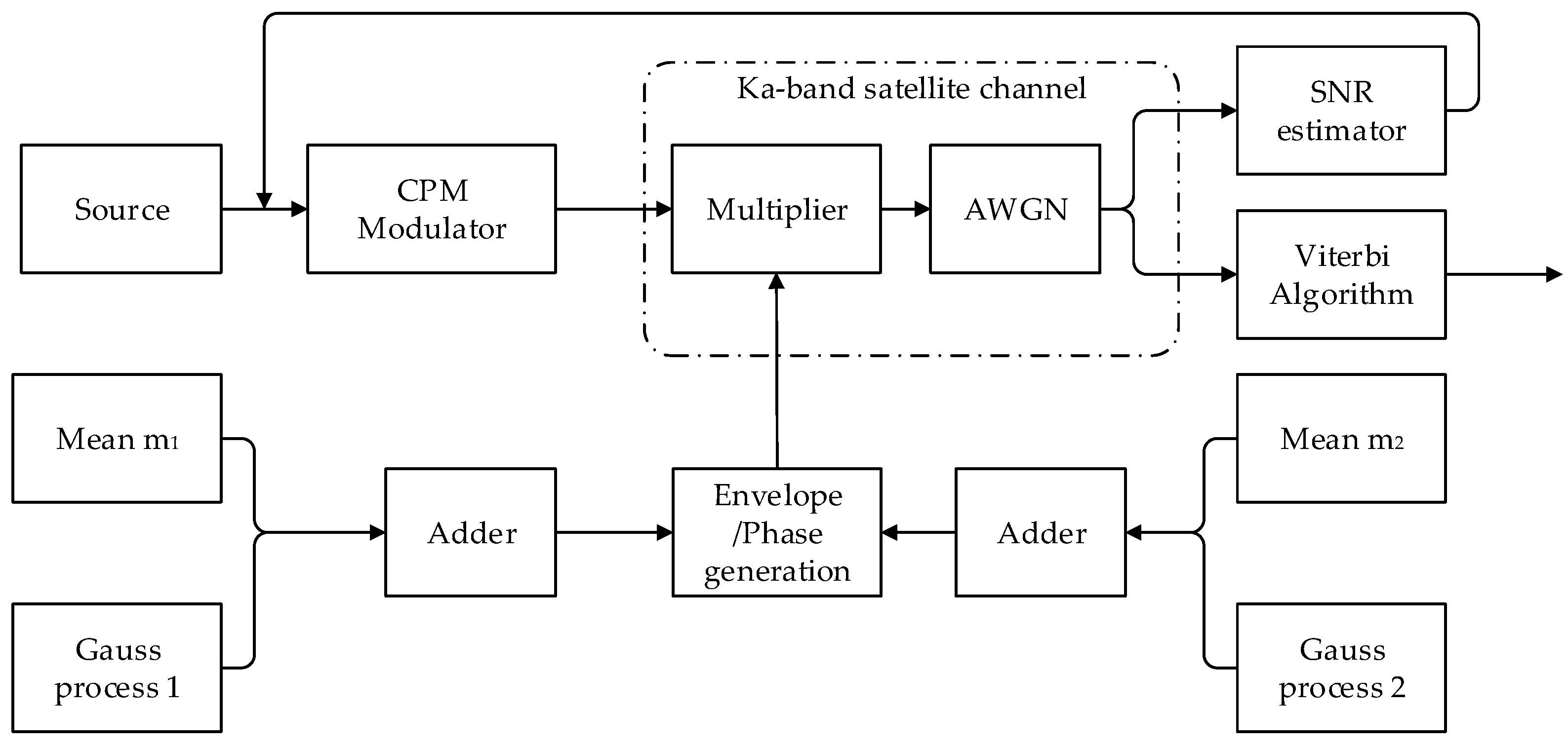
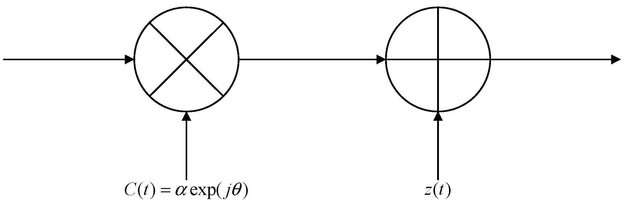
When transmitting a digital modulation signal $s(t)=\mathrm{Re}[s_1(t)\exp (j2\pi f_{c}t)]$ through the channel, $s_1(t)$ is the time domain complex baseband, and $s_1(f)$ is the frequency domain complex baseband. The equivalent lowpass signal (excluding AWGN) can be expressed as

$$r(t)={\displaystyle \underset{-\propto }{\overset{\propto }{\int }}C(f,t)s_1(f)\exp (j2\pi ft)df},$$

(8)

where $C(f,t)$ is the time-frequency transfer function of the channel that can be viewed as a complex value independent frequency in the signal bandwidth because the Ka-band fading channel is a non-frequency selective channel. Considering the spectrum of $s_1(f)$ concentrated in the vicinity of $f=0\mathrm{Hz}$, $C(f,t)=C(0,t)$ can be substituted into Formula (8)

$$\begin{array}{l}r(t)={\displaystyle \underset{-\infty }{\overset{\infty }{\int }}C(0,t)s_1(f)\exp (j2\pi ft)df}\\ =C(0,t){\displaystyle \underset{-\infty }{\overset{\infty }{\int }}{s}_1(f)\exp (j2\pi ft)df}\\ =C(0,t)s_1(t)\\ =\alpha (t)\exp (j\theta (t))s_1(t)\end{array}.$$

(9)

The fading characteristics can be regarded as a constant in a symbol interval because of the slow time-varying characteristics of multiplicative interference. Formula (9) can be simplified as

$$r(t)=\alpha \exp (j\theta )\cdot s_1(t)0\le t\le T,$$

(10)

where $T$ is the cycle of modulation symbol and $\alpha$ and $\theta$ are the envelope and phase of the equivalent lowpass channel, respectively. The researches show that the characteristics of a Ka-band satellite communication channel are determined mainly by the weather. The envelope and phase obey the Gauss distribution [24], and the probability density function can be expressed as

$$p(\alpha )=\frac{1}{\sqrt{2\pi }{\sigma }_1}\exp (-\frac{{(\alpha -m_1)}^2}{2{{\sigma }_1}^2})$$

(11)

$$p(\theta )=\frac{1}{\sqrt{2\pi }{\sigma }_2}\exp (-\frac{{(\theta -m_2)}^2}{2{{\sigma }_2}^2}),$$

(12)

where, ${\sigma }_1$, ${\sigma }_2$, $m_1$, and $m_2$ are available in

Table 1. Ka-band satellite channel envelope and phase model.

Weather Conditions	${\mathit{m}}_1$	${{\mathit{\sigma }}_1}^2$	${\mathit{m}}_2$	${{\mathit{\sigma }}_2}^2$
Clear/cloudy	0.455	0.00056	0.0079	0.00381
Cumulus cloud	0.346	0.00272	0.0154	0.00864
Light rain	0.483	0.00003	0.0088	0.00546
Thunder shower	0.436	0.01386	0.0068	0.00414
Blowing snow	0.500	0.00021	0.0089	0.00435
Ice pellets	0.482	0.00062	0.0094	0.00544
Rain	0.662	0.02000	−0.0089	0.03077

.

Table 1 shows the probability distribution parameters of the signal envelope and phase under various weather conditions in a Ka-band satellite communication channel [24]. Where, ${\sigma }_1$ and ${\sigma }_2$ are the variances of the signal envelope and phase, respectively, $m_1$ and $m_2$ are the mean of the signal envelope and phase, respectively. Previous studies have accumulated a considerable amount of data from many propagation characteristic measurement experiments in Olympus-star, Italsat-star and ACTS-star [24,25], the values in Table 1 is thus obtained.

Through the above analysis, we can establish the Ka-band satellite communication channel statistical model as shown in Figure 1. The digital modulation signal can be expressed as a result of the frequency independent complex multiplicative interference factor and AWGN after the non-frequency selective fading channel. $C(t)=\alpha \exp (j\theta )$ is the channel multiplication vector, and $z(t)$ is the AWGN.

3. System Model

The Ka-band satellite channel can be simulated by a multiplicative interference vector $C(t)$ and $z(t)$ from Section 2. The schematic of the system can be established as shown in Figure 2.

The data source produces a binary sequence. The data symbol generated at any time is independent of the previous symbol. The probability of the two symbols is the same. The information was sequenced through the CPM modulator and transmitted to the Ka-band fading channel. Gaussian Processes 1 and 2 in Figure 2 are considered as two independent stochastic processes with a mean of zero, and the variances are ${\sigma }_1$ and ${\sigma }_2$. Gaussian process 1 and the real constant generator 1 are added to generate the Gaussian stochastic process $\alpha$. Gaussian stochastic process $\theta$ can be generated in the same way. $\theta$ is sent to the exponential generator and multiplied with $\alpha$ to obtain the multiplicative interference vector $C(t)=\alpha \exp (j\theta )$. Different weather conditions only need to change the variance and the mean of $\alpha$ and $\theta$. The received signal can be represented as $r(t)$ (the expression is shown in follows) after the Ka-band fading channel. The SNR is estimated according to the received signal and the SNR estimators are shown in Section 4. A suitable coded modulation scheme is selected in the feedback link according to the value of SNR and the ACM schemes switching standards (Since the emphasis of this paper is on SNR estimators, we do not introduce too many coding process). The data is transmitted to the Ka-band fading channel according to the selected coded modulation scheme and the received signal is processed by Viterbi algorithm.

Transmitting terminal uses a complex-valued low-pass CPM signal, which is given by

$$\mathrm{s}(t,a)=\exp \left\{j\varphi (t,a)\right\},$$

(13)

where, for $nT\le t\le (n+1)T$

$$\varphi (t,a)=2\pi h{\displaystyle \sum _{i=0}^n{a}_i}q(t-iT),$$

(14)

where $T$ is the symbol time, $a=(a_0,a_1\cdots )$ is the transmitted information sequence, $h=K/P$ is the modulation index, where $K$ and $P$ are the coprime integer, and $q(t)$ is the phase pulse and is a continuous monotone function

$$q(t)=\{\begin{array}{c}0\\ 1/2\end{array}\begin{array}{c}t\le 0\\ t>LT\end{array}.$$

(15)

The CPM signal can be obtained by integrating the rectangular pulse (LREC) with a duration of $LT$, the raised cosine pulse (LRC), or the Gaussian minimum shift keying (GMSK) pulse and expressed as

$$q(t)={\displaystyle {\int }_{-\infty }^{t}g(\tau )},$$

(16)

where $g(t)$ is the pulse shaping function and is nonzero in $0\le t\le LT$. $g(t)$ is a full response when $L=1$ and a partial response when $L>1$. The received signal is given by

$$r(t)=As(t)+z(t),$$

(17)

where $A$ is the true amplitude of the received signal, $s(t)$ is the CPM modulation signal, and $z(t)$ is additive Gaussian white noise with the variance of ${\delta }^2$.

This paper aims to estimate the SNR according to the received signal. The signal fading caused by the envelope plays a decisive role, and signal fading caused by the phase is almost negligible. Therefore, the mean value of the envelope can be approximated as the multiplicative fading in the channel. In practical applications, the multiplication factor $m_1$ of the channel when the weather condition is different can be determined according to Table 1. The power of the transmission signal can be expressed as

$$S={(\frac{A}{m_1})}^2.$$

(18)

The average SNR for Ka-band fading channels can be expressed as

$$\begin{array}{l}SNR=10{\log }_{10}(\frac{S}{N})\\ =10{\log }_{10}(\frac{A^2}{{m_1}^2{\delta }^2})\end{array}.$$

(19)

4. SNR Estimators

After sampling the received signal in Formula (16), the output sequence is expressed as

$$r_k=A{s}_k+z_{k}k=1,2,\cdots ,K,$$

(20)

where $K$ is the observation point after sampling, $r_k$ obeys the Gauss distribution, $A{s}_k$ is the mean, and ${\delta }^2$ is the variance.

4.1. DA ML Estimator

The probability density function of the received sequence in Formula (20) is

$$p(r_k)=\frac{1}{\sqrt{2\pi }\delta }\exp (-\frac{{(r_k-A{s}_k)}^2}{2{\delta }^2}).$$

(21)

Given the statistical independence in sampling, Formula (21) can be expressed as

$$p(r)={(\frac{1}{2\pi {\delta }^2})}^{K/2}\exp (-{\displaystyle \sum _{k=1}^K\frac{{(r_k-A{s}_k)}^2}{2{\delta }^2}}),$$

(22)

and the corresponding log-likelihood function is

$$\ln p(r)=-\frac{K}{2}\ln 2\pi {\delta }^2-\frac{1}{2{\delta }^2}{\displaystyle \sum _{k=1}^K{(r_k-A{s}_k)}^2}.$$

(23)

The partial derivative of $A$ and ${\delta }^2$ is respectively set as

$$\frac{\partial \ln p(r)}{\partial A}=\frac{1}{{\delta }^2}{\displaystyle \sum _{k=1}^K(r_k-A{s}_k)}{s}_k$$

(24)

and

$$\frac{\partial \ln p(r)}{\partial {\delta }^2}=\frac{1}{2{\delta }^4}{\displaystyle \sum _{k=1}^K{(r_k-A{s}_k)}^2}-\frac{K}{2{\delta }^2}.$$

(25)

where, $\ln p(r)$ has a maximum value if the result is zero. $A$ and ${\delta }^2$ can be expressed, respectively as

$${\widehat{A}}_{ML}=\frac{{\displaystyle \sum _{k=1}^K{r}_k*s_k}}{{\displaystyle \sum _{k=1}^K{s}_k*s_k}}$$

(26)

and

$${{\widehat{\delta }}_{ML}}^2=\frac{{\displaystyle \sum _{k=1}^K{(r_k-{\widehat{A}}_{ML}{s}_k)}^2}}{K}.$$

(27)

The SNR estimate is computed using

$$SNR=10{\log }_{10}(\frac{{{\widehat{A}}_{ML}}^2}{{m_1}^2{{\widehat{\delta }}_{ML}}^2}).$$

(28)

4.2. M₂M₄ Estimator

The DA ML estimator requires the receiver and prior information sequences of the transmitter. However, obtaining prior information is impossible in some cases of practical application. This paper presents the M₂M₄ estimation method without prior information sequence. The two-order moments and four-order moments of the received sequence in Formula (20) can be expressed as

$$M_2=E[r_k{r_k}^{\ast }]=A^{2}E[{\left|s_k\right|}^2]+AE[s_k{z_k}^{\ast }]+AE[{s_k}^{\ast }{z}_k]+E[{\left|z_k\right|}^2]$$

(29)

and:

$$\begin{array}{l}{M}_4=E[{(r_k{r_k}^{\ast })}^2]=A^{4}E[{\left|s_k\right|}^4]+2A^3(E[{\left|s_k\right|}^2{s}_k{z_k}^{\ast }]+E[{\left|s_k\right|}^2{s_k}^{\ast }{z}_k])+\\ A^2(E[{(s_k{z_k}^{\ast })}^2]+4E[{\left|s_k\right|}^2{\left|z_k\right|}^2]+E[{({s_k}^{\ast }{z}_k)}^2])+\\ 2A(E[{\left|s_k\right|}^2{s}_k{z_k}^{\ast }]+E[{\left|z_k\right|}^2{s_k}^{\ast }{z}_k])+E[{\left|z_k\right|}^4]\end{array}$$

(30)

where, the conjugate of $r_k$, $s_k$ and $z_k$ are denoted ${r_k}^{\ast }$, ${s_k}^{\ast }$ and ${z_k}^{\ast }$.

Given that the signal and noise are independent of each other, and the mean is zero, Equations (29) and (30) can be simplified as follows

$$M_2=A^2+{\delta }^2$$

(31)

and

$$M_4=A^4+4A^2{\delta }^2+2{\delta }^4.$$

(32)

The estimated value of $A$ and ${\delta }^2$ can be expressed as

$${{\widehat{A}}_{MM}}^2=\sqrt{2{(M_2)}^2-M_4}$$

(33)

and

$${{\widehat{\delta }}_{MM}}^2=M_2-{{\widehat{A}}_{MM}}^2.$$

(34)

The corresponding SNR estimator is

$$SNR=10{\log }_{10}(\frac{{{\widehat{A}}_{MM}}^2}{{m_1}^2{{\widehat{\delta }}_{MM}}^2}).$$

(35)

$M_2$ and $M_4$ can be obtained in practical applications through the average value of the receiving sequence and expressed respectively as

$$M_2=\frac{1}{K}{\displaystyle \sum _{k=1}^K{\left|r_k\right|}^2}$$

(36)

and

$$M_4=\frac{1}{K}{\displaystyle \sum _{k=1}^K{\left|r_k\right|}^4}.$$

(37)

4.3. Performance Index

Two estimators are simulated in the MATLAB simulation platform and the SNR fitting curve is drawn. The abscissa is the SNR value of the theory. The ordinate is the SNR value of the estimate, which can determine whether the SNR estimators are unbiased. The main index to measure the performance of SNR estimators in the simulation is NMSE, which can be expressed as

$$NMSE(\widehat{\rho })=\frac{E[{(\widehat{\rho }-\rho )}^2]}{{\rho }^2},$$

(38)

where $\rho$ is the SNR value of the theory and $\widehat{\rho }$ is the SNR value of the estimate. The estimator performs better when the NMSE is smaller.

The CRLB provides absolute lower limit of the estimation. The NMSE can be compared with the CRLB to illustrate the absolute performance of the estimator. A parameter vector $\mathsf{\beta }={[SN]}^T$ is defined as the relationship between SNR, and the parameter vector is

$$g(\mathsf{\beta })=\rho =\frac{S}{N},$$

(39)

where $S={(\frac{A}{m_1})}^2$ is the signal power and $N={\delta }^2$ is the noise power. The formula given by Kay in Reference [26] shows that

$$\mathrm{var}(\rho )\ge \frac{\partial g(\mathsf{\beta })}{\partial \mathsf{\beta }}{I}^{-1}(\mathsf{\beta })\frac{\partial g{(\mathsf{\beta })}^T}{\partial \mathsf{\beta }},$$

(40)

where $\frac{\partial g(\mathsf{\beta })}{\partial \mathsf{\beta }}{I}^{-1}(\mathsf{\beta })\frac{\partial g{(\mathsf{\beta })}^T}{\partial \mathsf{\beta }}$ is the CRLB. $I(\mathsf{\beta })$ is the Fisher Information Matrix, which can be expressed as

$$I(\mathsf{\beta })=\left[\begin{array}{cc}-E(\frac{{\partial }^2\ln p(r)}{\partial S^2})& -E(\frac{{\partial }^2\ln p(r)}{\partial S\partial N})\\ -E(\frac{{\partial }^2\ln p(r)}{\partial N\partial S})& -E(\frac{{\partial }^2\ln p(r)}{\partial N^2})\end{array}\right].$$

(41)

When the SNR is low (0–6 dB), the NDA CRLB is higher than DA CRLB; however, the two lower bounds tend to coincide with the increase of SNR (greater than 6 dB) [27]. The CRLB of the DA SNR estimation is simple and unaffected by the shaping filter and sampling. Thus, this study uses DA CRLB as the reference of absolute performance. The CRLB of the complex signal can be expressed as [28]

$$NMSE(\widehat{\rho })\ge \frac{1}{K}(\frac{2}{\rho }+1).$$

(42)

MATLAB tools are used to simulate and analyze the above theoretical models. The data source produces a binary sequence and sequenced through the CPM modulator. Transmitted the modulation signal to the Ka-band fading channel in a number of frames in the range of SNR. Seven weather conditions are generated according to the numerical information in Table 1. After the fading factor is obtained, the fading channel simulation model is established by using the theoretical channel model in Section 2. The SNR is estimated according to Formulas (28) and (35) in Section 4. Numerical results and simulation performance are shown in Section 5.

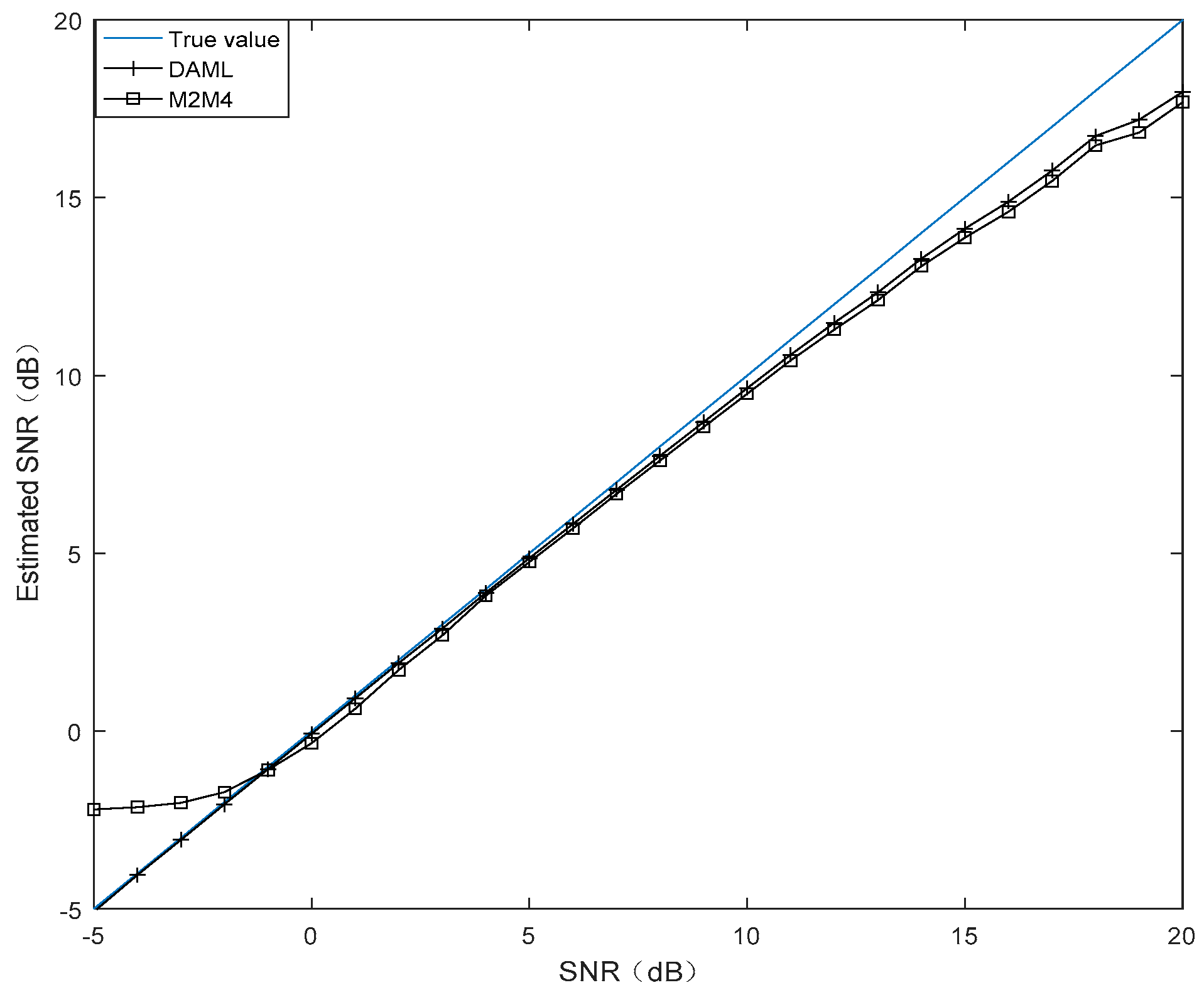
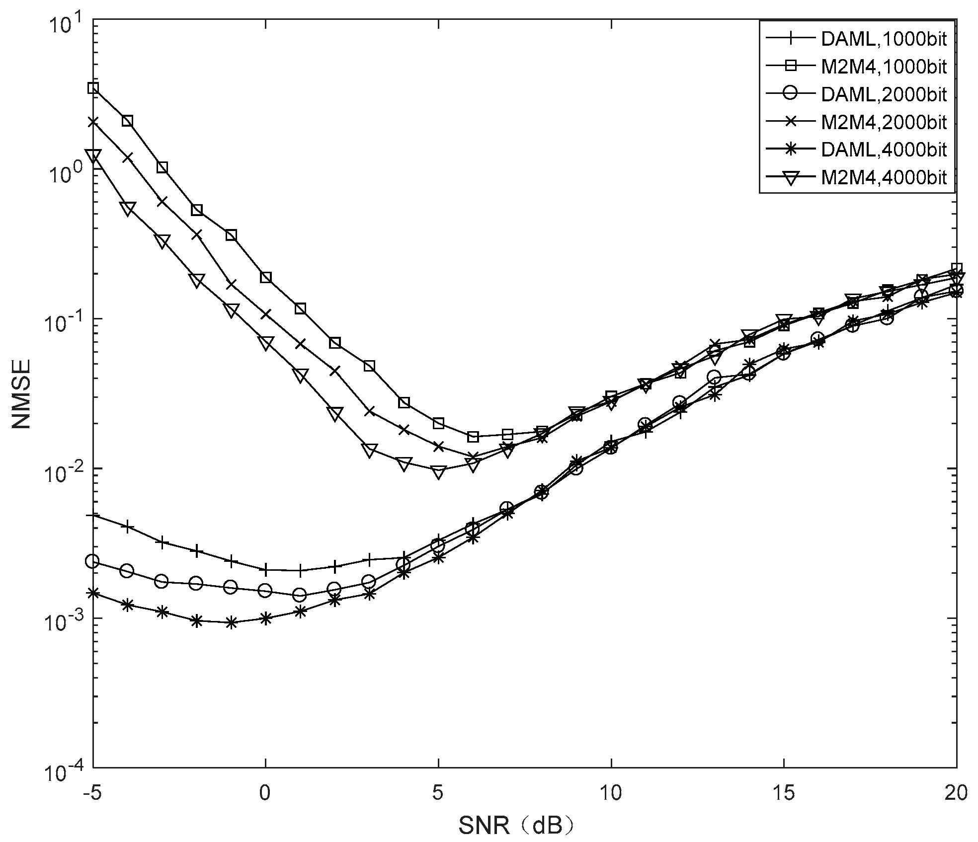
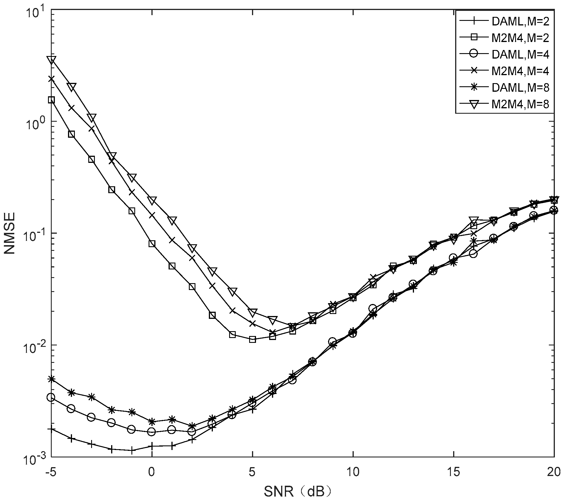
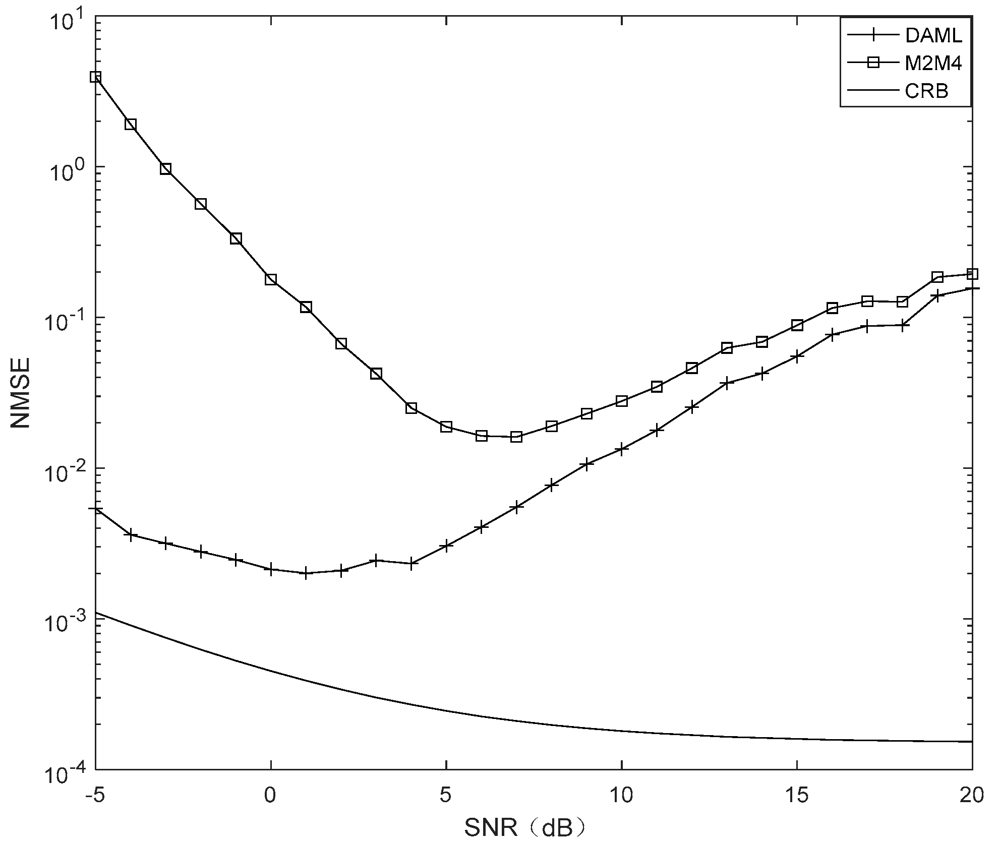
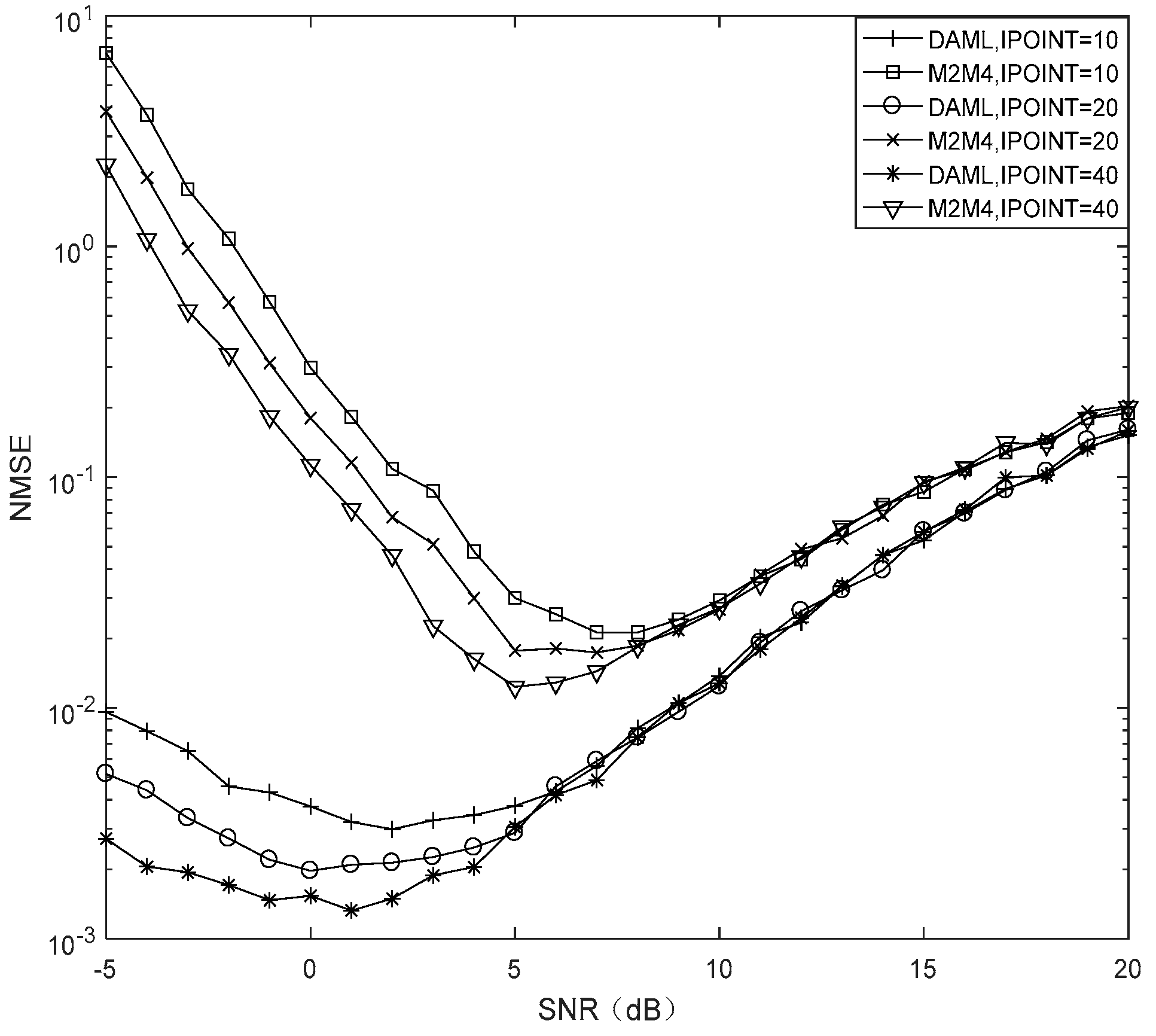
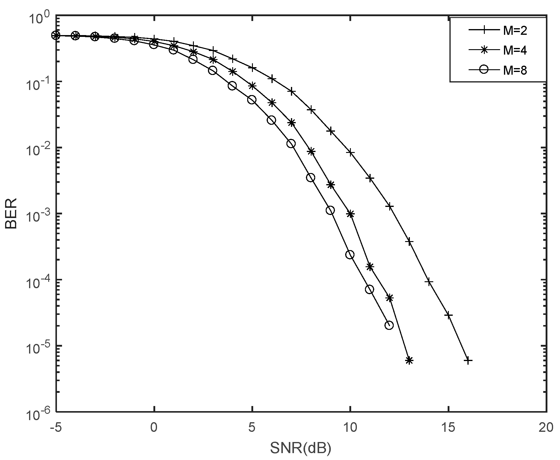
5. Numerical Results and Analysis

The length of the source information sequence is set to 1000 bits, and the sampling points per symbol are set to IPOINT = 20. For the CPM modulator, the modulation index is set to h = 1/4, the pulse shaping function is set to GMSK, L = 2, and the modulation order is set to M = 8. The average value of the SNR estimators is calculated with 1000 frames.

The SNR fitting curve of the DA ML and M₂M₄ estimators are shown in Figure 3. The horizontal axis in the figure is shown as the actual SNR, which is the assumed value in the MATLAB simulation and is the channel environment in the actual communication. The ordinate is the SNR estimated by the Formulas (28) and (35) in Section 4. The horizontal and ordinate of the truth values are all the actual values of SNR and the true values are the standard used to measure the offset of estimate SNR and actual SNR. The DA ML estimator can be approximated as unbiased when SNR is less than 5 dB. The estimation error is large in the case of medium and high SNR. The estimation bias increases with the increase of SNR. The M₂M₄ estimator can be approximated as unbiased when SNR is medium (near 5 dB), but the estimation error is significantly large at low and high SNRs.

The NMSE of the DA ML and M₂M₄ estimators are shown in Figure 4. The DA ML estimator has the best performance when SNR is approximately 0 dB, but the performance becomes worse with the increase of SNR. The M₂M₄ estimator has the best estimation performance when SNR is near 7 dB. The performance curve of the M₂M₄ estimator is similar to a parabola, and the performance is poor at low SNR. The performance becomes worse with the increase of SNR after 7 dB. The two estimators cannot achieve the Cramer-Rao bounds and the existence of the SNR node. The performance worsens with the increase of SNR after the node because the non-CM characteristics introduced by the fading factor. When the SNR is low, the noise power is the main factor affecting the estimation performance due to the large noise power, while the signal power is the main factor affecting the estimation performance in the medium to high SNR. In the process of signal power estimation, it is necessary to do the division of the mean of the fading factor as in Formulas (18). The difference between the estimated value and actual value of the signal power is greater with the increase of SNR, which will lead to the worse performance. The DA ML estimator displays better performance than the M₂M₄ estimator, especially in the low SNR. The performance gap between the two estimators is reduced gradually when the SNR is medium or high. The two estimators are close to each other in practical applications when the channel environment is good. Thus, the M₂M₄ estimator can be used to reduce the complexity. The DA ML estimator can be used to improve the estimation performance when the channel environment is poor, and the transmitter information sequence is known.

Three parameters affect the estimation performance by setting the different values of the parameters. These parameters include the number of sampling points per symbol, the length of the transmitted information sequence, and the modulation order. The common parameters are the same as the previous settings.

The NMSEs of DA ML and M₂M₄ for IPOINT = 10, 20, 40 are plotted in Figure 5. The estimation performance improves with the increase in the number of sampling points per symbol.

The NMSEs of DA ML and M₂M₄ for the length of transmission information for 1000, 2000, and 4000 bits are plotted in Figure 6. The estimation performance improves the longer the transmitted information.

The NMSEs of DA ML and M₂M₄ for M = 2, 4, 8 are plotted in Figure 7. The estimation performance improves as the CPM modulation order becomes smaller.

The three figures show that the three parameters have no influence on the estimation performance when SNR is greater than 8 dB. The observation points of the receiver can be expressed as

$$K=\frac{length(bit)*IPOINT}{{\log }_2(M)}.$$

(43)

We can obtain the conclusion by considering the three parameters. The more observation points the receiver has, the better the two estimators performs. The number of observation points has no influence on the estimation performance when the SNR is greater than 8 dB. When the channel environment is poor in practical applications, better estimation performance can be obtained by increasing the number of sampling points per symbol, increasing the length of the transmitted information sequence, and reducing the CPM modulation order.

SNR estimators are the main research content of this paper, and we only select the modulation orders as the example to illustrate the principle of ACM control loop. The length of the source information sequence is set to 1000 bit, and the sampling points per symbol are set to IPOINT = $10*{\log }_2(M)$. For the CPM modulator, the modulation index is set to h = 1/2, the pulse shaping function is set to RC, L = 2, and the modulation orders are set to M = 2, 4, 8, respectively. The average value of the SNR estimators is calculated with 1000 frames.

The BER for different modulation orders are shown in Figure 8. For the same SNR, the BER of the system decreases as the modulation order becomes larger. The target BER is assumed to be 10⁻⁴. When the SNR is less than 10.6 dB, all the three modulation orders can’t achieve the target BER, we can choose a low BER method as the modulation order of the system, that is M = 8. When the SNR is within the range of 10.6 dB to 11.4 dB, only M = 8 can achieve the target BER, so we still choose M = 8 as the modulation order of the system. When SNR is in the range of 11.4 dB to 14 dB, both M = 4 and M = 8 can achieve the target BER. Because of the higher frequency band utilization rate of M = 4, we select M = 4 as the modulation order of the system. When the SNR is greater than 14 dB, all the three modulation orders can achieve the target BER. Because of the highest frequency band utilization in M = 2, we select M = 2 as the modulation order of the system. When SNR grows the modulation order is decreased by the ACM control loop, when SNR drops down higher modulations have to be used.

6. Conclusions

ACM technology is one of the effective measures to resist rain attenuation in Ka-band satellite communication. The accuracy of SNR estimation is one of the main factors that affect the performance of the ACM system. This paper establishes the channel model of Ka-band satellite communication, and derives and analyzes the DA ML and M₂M₄ estimators for the SNR of CPM in Ka-band fading channel. The SNR fitting curve, NMSE, and CRLB were used as indices for analysis of the performance of the two estimators. The two estimators cannot achieve the CRLB, and the estimation performance in the medium and high SNR worsens with the increase of SNR. When the SNR is low, the performance of the DA ML estimator is better than the M₂M₄ estimator. The higher the number of observation points, the better the estimation performance of the two. When the SNR is high, the two estimators have similar estimation performance, and the observation points have no influence on the estimation performance. The two estimators in the commonly used SNR range have a better estimation performance and can be approximated as unbiased. Therefore, CPM can be a competitive modulation mode of the ACM technology in Ka-band satellite communication.

References

1. Rossi, T.; de Sanctis, M.; Ruggieri, M. Satellite communication and propagation experiments through the alphasat Q/V band Aldo Paraboni technology demonstration payload. IEEE Aerosp. Electron. Syst. Mag. 2016, 31, 18–27. [Google Scholar] [CrossRef]
2. Cianca, E.; Rossi, T.; Yahalom, A. EHF for satellite communications: The new broadband frontier. Proc. IEEE 2011, 99, 1858–1881. [Google Scholar] [CrossRef]
3. Dai, C.Q.; Huang, N.N.; Chen, Q. Adaptive transmission scheme in Ka-band satellite communications. In Proceedings of the 2016 IEEE International Conference on Digital Signal Processing, Beijing, China, 16–18 October 2016; pp. 336–340. [Google Scholar]
4. Ojo, J.S.; Owolawi, P.A. Application of synthetic storm technique for diurnal and seasonal variation of slant path Ka-band rain attenuation time series over a subtropical location in South Africa. Int. J. Antennas Propag. 2015. [Google Scholar] [CrossRef]
5. Luini, L.; Capsoni, C. Prediction of monthly rainfall statistics from data with long integration time. Electron. Lett. 2013, 49, 1104–1106. [Google Scholar] [CrossRef]
6. Shrestha, S.; Nadeem, I.; Kim, S.; Han, S.; Choi, D. Rain Specific Attenuation and Frequency Scaling approach in Slant-Path for Ku and Ka-Band Experiments in South Korea. In Proceedings of the 16th International Conference on Electronics, Information, and Communication, Phuket, Thailand, 11–14 January 2017. [Google Scholar]
7. Kourogiorgas, C.; Panagopoulos, A.D. A rain-attenuation stochastic dynamic model for LEO satellite systems above 10 GHz. IEEE Trans. Veh. Technol. 2015, 64, 829–834. [Google Scholar] [CrossRef]
8. Yang, Z.; Li, H.; Jiao, J. CFDP-based two-hop relaying protocol over weather-dependent Ka-band space channel. IEEE Trans. Aerosp. Electron. Syst. 2015, 51, 1357–1374. [Google Scholar] [CrossRef]
9. Zain, A.F.M.; Albendag, A.A.M. Improving ITU-R rain attenuation model for HAPS earth-space link. In Proceedings of the 2013 IEEE International Conference on Space Science and Communication, Melaka, Malaysia, 1–3 July 2013; pp. 56–59. [Google Scholar]
10. Shrestha, S.; Choi, D. Characterization of Rain Specific Attenuation and Frequency Scaling Method for Satellite Communication in South Korea. Int. J. Antennas Propag. 2017. [Google Scholar] [CrossRef]
11. Shrestha, S.; Choi, D. Study of rain attenuation in Ka band for satellite communication in South Korea. J. Atmos. Sol. Terr. Phys. 2016, 148, 53–63. [Google Scholar] [CrossRef]
12. Shrestha, S.; Choi, D. Study of 1-min rain rate integration statistic in South Korea. J. Atmos. Sol. Terr. Phys. 2017, 155, 1–11. [Google Scholar] [CrossRef]
13. Shrestha, S.; Park, J.J.; Choi, D.Y. Rain rate modeling of 1-min from various integration times in South Korea. SpringerPlus 2016, 51, 433. [Google Scholar] [CrossRef] [PubMed]
14. Acquisition, Presentation and Analysis of Data in Studies of Radio Wave Propagation. Available online: https://www.itu.int/dms_pubrec/itu-r/rec/p/R-REC-P.311-16-201609-I!!PDF-E.pdf (accessed on 29 June 2017).
15. Usha, S.M.; Nataraj, K.R. Bit Error Rate Analysis Using QAM Modulation for Satellite Communication Link. Procedia Technol. 2016, 25, 456–463. [Google Scholar] [CrossRef]
16. Cariolaro, G. A system-theory approach to decompose CPM signals into PAM waveforms. IEEE Trans. Commun. 2010, 58, 200–210. [Google Scholar] [CrossRef]
17. Cariolaro, G.; Erseghe, T.; Laurenti, N. New Results on the Spectral Analysis of Multi-h CPM Signals. IEEE Trans. Commun. 2011, 59, 1893–1903. [Google Scholar] [CrossRef]
18. Wiesel, A.; Goldberg, J.; Messer, H. Non-data-aided signal-to-noise-ratio estimation. In Proceedings of the IEEE International Conference on Communications, New York, NY, USA, 28 April–2 May 2002; pp. 197–201. [Google Scholar]
19. Rice, M. Data-Aided and Non-Data-Aided Maximum Likelihood SNR Estimators for CPM. IEEE Trans. Commun. 2015, 63, 4244–4253. [Google Scholar] [CrossRef]
20. Chang, L.; Li, G.Y.; Li, J. Closed-Form SNR Estimator for MPSK Signals in Nakagami Fading Channels. IEEE Trans. Veh. Technol. 2016, 65, 6878–6887. [Google Scholar] [CrossRef]
21. Wu, H.; Sha, Z.C.; Huang, Z.T. Signal-to-noise ratio estimation for DVB-S2 based on eigenvalue decomposition. Commun. IET 2016, 10, 1–7. [Google Scholar] [CrossRef]
22. Li, Z.; Yang, D.; Wang, H. Maximum likelihood SNR estimator for coded MAPSK signals in slow fading channels. In Proceedings of the 2013 International Conference on Wireless Communications and Signal Processing, Hangzhou, China, 24–26 October 2013; pp. 1–6. [Google Scholar]
23. Matricciani, E.; Riva, C. Evaluation of the feasibility of satellite systems design in the 10–100 GHZ frequency range. Int. J. Satell. Commun. 1998, 16, 237–247. [Google Scholar] [CrossRef]
24. Loo, C. Impairment of digital transmission through a Ka band satellite channel due to weather conditions. Int. J. Satell. Commun. Netw. 1998, 16, 137–145. [Google Scholar] [CrossRef]
25. Loo, C. Statistical models for land mobile and fixed satellite communications at Ka band. In Proceedings of the Vehicular Technology Conference, Atlanta, GA, USA, 28 April–1 May 1996; pp. 1023–1027. [Google Scholar]
26. Kay, S.M.M. Fundamentals of Statistical Signal Processing, Volume I: Estimation Theory; Prentice Hall Press: Upper Saddle River, NJ, USA, 1993. [Google Scholar]
27. Alagha, N.S. Cramer-Rao bounds of SNR estimates for BPSK and QPSK modulated signals. IEEE Commun. Lett. 2001, 5, 10–12. [Google Scholar] [CrossRef]
28. Pauluzzi, D.R.; Beaulieu, N.C. A comparison of SNR estimation techniques for the AWGN channel. IEEE Trans. Commun. 2000, 48, 1681–1691. [Google Scholar] [CrossRef]
Figure 1. Ka-band satellite channel statistical model.
Information 08 00075 g001
Figure 2. Schematic of the system.
Information 08 00075 g002
Figure 3. Estimated SNR comparison of DA ML and M2M4 in Ka-band fading channel.
Information 08 00075 g003
Figure 4. NMSE comparison of DA ML and M2M4 in Ka-band fading channel.
Information 08 00075 g004
Figure 5. NMSE comparison of DA ML and M2M4 in different IPOINT.
Information 08 00075 g005
Figure 6. NMSE comparison of DA ML and M2M4 in different lengths of information.
Information 08 00075 g006
Figure 7. NMSE comparison of DA ML and M2M4 in different M.
Information 08 00075 g007
Figure 8. BER in different M.
Information 08 00075 g008