Enhancement of Low Contrast Images Based on Effective Space Combined with Pixel Learning

Abstract

Images captured in bad conditions often suffer from low contrast. In this paper, we proposed a simple, but efficient linear restoration model to enhance the low contrast images. The model’s design is based on the effective space of the 3D surface graph of the image. Effective space is defined as the minimum space containing the 3D surface graph of the image, and the proportion of the pixel value in the effective space is considered to reflect the details of images. The bright channel prior and the dark channel prior are used to estimate the effective space, however, they may cause block artifacts. We designed the pixel learning to solve this problem. Pixel learning takes the input image as the training example and the low frequency component of input as the label to learn (pixel by pixel) based on the look-up table model. The proposed method is very fast and can restore a high-quality image with fine details. The experimental results on a variety of images captured in bad conditions, such as nonuniform light, night, hazy and underwater, demonstrate the effectiveness and efficiency of the proposed method.

1. Introduction

In the image acquisition process, the low illumination in nonuniformly illuminated environment or light scattering caused by turbid medium in the foggy/underwater environment will lead to low image contrast. Based on the variety of bad conditions, however, it is difficult to enhance the image of these conditions through a unified approach. Though traditional methods such as the histogram equalization will deal with all these low contrast images, most results are show to be uncomfortable for the human visual system. Therefore, most of them establish a specific recovery model based on the distinctive physical environment to enhance the images.

Dealing with light compensation is usually done by using the Retinex (retina-cortex) model, which is built on the human visual system [1,2,3]. The early single-scale Retinex algorithm proposed by Jobson [4] can either provide dynamic range compression on a small scale or tonal rendition on a large scale. Therefore, Jobson continued his research and proposed the MSR (multiscale Retinex) algorithm [5], which has been the most widely used in recent years. Most improved Retinex algorithms [6,7,8,9,10,11,12,13,14,15] are based on MSR. However, the Gaussian filtering used by the MSR algorithm calculates a large number of floating data, which makes the algorithm take too much time. Therefore, for practical use, Jiang et al. [15] used hardware acceleration to implement the MSR algorithm. In addition, some research [16] used the dehaze model instead of the Retinex model to deal with the negative input image for light compensation or using the bright channel prior with the guided filter [17] for a quick lighting compensation.

Early haze removal algorithms require multiple frames or additional depth map information [18,19,20]. Since Fattal et al. [21] and Tan et al. [22] proposed a single-frame dehaze algorithm relying on stronger priors or assumptions, the single-frame dehaze algorithms have become a research focus. Subsequently, He et al. [23] proposed the DCP (dark channel prior) for haze removal, which laid the foundation for the dehazing algorithm in recent years. Combining the DCP with the guided filter [24] is also the most efficient method for the dehazing algorithm. Since then, the principal study of the fog algorithm has focused on the matting technique of transmittance [24,25,26,27,28,29,30]. Meng et al. [25] applied a weighted L1-norm-based contextual regularization to optimize the estimation of the unknown scene transmission. Sung et al. [26] used a fast guided filter that was combined with the up/down samples to optimize the performance time. Zhang et al. [28] used the five-dimensional feature vectors to recover the transmission values by finding their nearest neighbors from the fixed points. Li et al. [30] computed a spatially varying atmospheric light map to predict the transmission and refined it by the guided filter [24]. The guided filter [24] is an O(n) time edge-preserving filter with the similar result of bilateral filter. However, in the application, the well-refined methods are hard to perform on a video system due to the time cost, and the fast local filters like guided/bilateral filters would concentrate the blurring near the strong edges, then introducing halos.

There have been several attempts to restore and enhance the underwater image [31,32,33]. However, there is no general restoration model for such degraded images. Research mainly applies the white balance [32,33,34] to correct the color bias at first and then uses a series of contrast stretch processing to enhance the visibility of underwater images.

Although these studies have applied different models and methods for image enhancement, the essential goal of all of these is to stretch the contrast. In this paper, we proposed a unified restoration model for these low-contrast degraded images to reduce the human operations or even in some multidegradation environments. Moreover, due to the artifacts produced by the patch-based methods we applied in our approach, the pixel learning refinement is proposed.

2. Background

2.1. Retinex Model

The Retinex theory was proposed by Land et al. based on the property of the human visual system, which is commonly referred to as the color constancy. The main goal of this model is to decompose the given image I into the illuminated image L and the reflectance image R. Then, the output of the reflectance image R is its result. The basic Retinex model is given as:

$$I(x)=L(x).*R(x),$$

(1)

where x is the image coordinates and operator .* denotes the matrix point multiplication. The main parameter of the Retinex algorithm is the Gaussian filter’s radius. A large radius can get obtain color recovery, and a small radius can retain more details. Therefore, the most commonly used Retinex algorithm is multiscale. Early research on Retinex was mainly for light compensation. In recent years, a large number of studies has been undertaken to enhance the image with hazy [10] and underwater images [8,31] using the Retinex algorithm. However, these methods are developed with their own framework for a specific environment.

2.2. Dehaze Model

The most widely-used dehaze model in computer vision is:

$$I(x)=J(x).*T(x)+(1-T(x))\times A,$$

(2)

where I is the hazy image, J is the clear image, T is the medium transmittance image and A is the global atmospheric light, usually constant. In the methods of estimating the transmittance image T, the DCP is the simplest and most widely-used method, which is given by:

$$\begin{array}{l}dar{k}_p(I(x))=\underset{c\in (r,g,b)}{\min }(I_c(x))\\ dar{k}_b(I(x))=\underset{y\in \Omega (x)}{\min }(dar{k}_p(I(y)))\end{array},$$

(3)

where dark_p represents the pixel dark channel operator and dark_b represents the block dark channel operator. I is the input image; x is the image coordinates; c is the color channel index; and $y\in \Omega (x)$ indicates that y is a local patch centered at x. The main property of the block dark channel image is that in the haze-free image, the intensity of its block dark channel image tends to be zero. Assuming that the atmospheric light A is given, the estimated expression of the transmittance T can be obtained by putting the block dark channel operator on both sides of (2):

$$T(x)=1-dar{k}_b(\frac{I(x)}{A}),$$

(4)

With transmittance T and the given atmospheric light A, we can enhance the hazy image according to Equation (2). However, Equation (4) can only be used as a preliminary estimation because the block dark channel image can produce the block artifacts due to the minimum filtering. Therefore, a refine process is required before the recovery. In addition, the dehaze model has some physical defects that can result in the image looking dim after haze removal.

In the next section, we present a simple linear model for enhancing all the mentioned low contrast images based on an observation of the images’ 3D surface graph.

3. Proposed Model

3.1. Enhance Model Based on Effective Space

The effective space comes from the observation of the 3D surface graph of the images. The three coordinate axes of the 3D surface graph are the image width (x-axis), the image height (y-axis) and the pixel value (z-axis), and all the pixel points of an image can be connected to form a surface, which is the 3D surface graph. In this paper, we call the minimum space of the 3D surface graph an effective space. In order to show the law of effective space, we transform the color images into gray scale and project their 3D surface graph on the x-z plane, as shown in Figure 1 (in the 2D projection, the x-axis is the image width, and the y-axis is the pixel value).

As can be seen, the projection of clear images is almost filled by the domain of the pixel value. On the contrary, the degraded images’ are compressed. Therefore, we assume that the proportion of the pixel value in the effective space denotes the detail information of the image. Since the image size is fixed in processing, we estimate the two smooth surfaces of the effective space that are the upper surface U (up) and the lower surface D (down) to obtain the proportion of the pixel value in the effective space. It should be noted that in the ideal clear image, U is a constant plane at 255, while D is zero. According to the relationship of the proportion, we can establish a linear model by:

$$\frac{I-D_I}{U_I-D_I}=\frac{J-D_J}{U_J-D_J}=\frac{J-0}{255-0},$$

(5)

where I represents the input degraded image, J represents the ideal clear image, U_I and U_J represent the upper surface of the effective space of I and J, respectively, and similarly, D_I and D_J represent the lower surface. Once we obtain U and D, we can enhance the low contrast images according to Equation (5). However, the denominator in Equation (5) can be zero when the pixel value of D is equal to U. Therefore, we introduce a small parameter in the denominator to avoid the division by zero. Our final enhanced model is given as:

$$J=U_J.*\frac{I-D_I}{U_I-D_I+\lambda },$$

(6)

where D is estimated by the block dark channel operation, according to Equation (3), U is estimated by the block bright channel operation, which can be calculated by Equation (3) with the min function replaced by the max function and λ is a small factor to prevent the division by zero, usually set to 0.01. U_J denotes the light intensity of the enhanced images, ideally set to the maximum gray level (the eight-bit image is 255). The images always looks dim after haze removal based on Equation (2). Our model can improve this phenomenon while combining the Retinex model and the dehaze model so that our model can be adapted according to the scene requirements.

3.2. Relationship with Retinex Model and Dehaze Model

If an image is haze free, the intensity of its block dark channel image is always very low and tends to zero. Similarly, if an image has abundant light supply, the intensity of its block bright channel image usually approaches the maximum value of the image dynamic range. The main cause of the dim restoration of the dehaze algorithm is the overestimated atmospheric light A. Considering a hazy image without color bias, the atmospheric light A is approximately equal in each channel of the color image; in other words, A_R = A_G = A_B. Due to this, Equation (4) can be rewritten as:

$$T=1-\frac{dar{k}_b(I)}{A},$$

(7)

where A represents the light intensity of all three channels. Putting Equation (7) into Equation (2), we can remove the haze with the style of our model as Equation (6):

$$J=\frac{I-A}{T}+A=\frac{I-A}{1-\frac{D_I}{A}}+A=A_J.*\frac{I-D_I}{A-D_I},$$

(8)

where, in our model, A_J denotes the illumination of the clear image and A is the input image’s illumination; whereas, in the fog model, A_J = A, which both represent the input image’s illumination. Due to the impact of the clouds, the light intensity is usually low when the weather is rainy or foggy. This can lead to the result of haze removal looking dim. On the other hand, most haze removal research assumes that the atmospheric light intensity is uniform, and A is estimated as a constant. According to Equation (9), if the input image has sufficient illumination, which means A = 255 = U_J = A_J, the proposed model is equivalent to the dehaze model. Nevertheless, the light intensity of a real scene is always nonuniform. As can be seen in Equation (9), when D_I remains the same, the larger the A we give, the smaller the J we have. On the whole, a large estimated value of the constant A will be great in the thick foggy region, but for the foreground region with only a little mist, it is too large. This is the main cause of haze removal always becoming a dim restoration. Moreover, if the input image I is a haze-free image, it will be the typical low contrast problem of Retinex. According to the constant zero tendency of the block dark channel image and Equation (1), we have a Retinex model with the style of Equation (6):

$$J=255\times R=255\times \frac{I}{L}=255\times \frac{I-0}{L-0}=255\times \frac{I-D_I}{L-D_I},$$

(9)

where $R\in \left[0,1\right]$ represents the reflectivity in Equation (1). In order to unify the dynamic range of the output image J, we multiply R by 255 of the eight-bit image. According to Equation (9), if we estimate the illuminated image L by a Gaussian filter, the proposed model is equivalent to the Retinex model. It is notable that the bright channel prior is also a good method to estimate L, and the bright channel prior will be faster than the Gaussian filter due to the integer operation. The study of Wang et al. [17] shows that the bright channel prior has a significant effect in terms of light compensation.

Due to the constant zero tendency of the block dark channel image, the proposed model will automatically turn into the Retinex model to compensate for the light intensity of the image in the haze-free region. Besides, the model mainly modified the two assumptions of the dehaze model that A_J is equal to A, and A is a constant; so that the proposed algorithm can increase the exposure of J when the input I is a hazy image. However, as a result of the use of the bright/dark channel prior, a refinement process is necessary to improve the block artifacts produced by the min/max filter used in the priors.

4. Pixel Learning for Refinement

4.1. Pixel Learning

Pixel learning (PL) is a kind of edge-preserving smoothing, which is similar to online learning. Generally, for the edge-preserving smoothing, the cost function is firstly established:

$$S(x)=\arg \min (\Vert I(x)-S(x)\Vert +\Vert \nabla S(x)\Vert ),$$

(10)

where S represents the process of smoothing and I represents the input image. In Equation (10), the first penalty term $\Vert I(x)-S(x)\Vert$ forces proximity between I and S, which can preserve the sharp gradient edges of I for S, and this will help reduce the artifacts, such as the haloes. The second penalty term $\lambda \times \Vert \nabla S(x)\Vert$ is the degree of similarity between the estimated component and the input image, and it forces the spatial smoothness on the processed image S. In the previous research results, there were a number of methods to solve the optimization problem of Equation (10), in which the most practical of the methods was the guided filter [24]. However, [24] still retained the halo artifacts due to the frequent use of the mean filter. Although, there are some improvements such as applying iteration optimization [27] or solving the equation of higher-order [24] to optimize the model, these algorithms are usually too time consuming for a practical use due to the large number of pixels in an input image as training examples for an optimization problem. Therefore, we introduce the idea of online learning to overcome the time-consuming process of optimization.

Online learning is different from batch learning. Its samples come in sequence; in other words, a one-by-one processing. Then, the classifier is updated according to each new sample. If the input samples are large enough, the online learning can converge in only one scanning. As an online learning technique, the pixel learning outputs the results pixel-by-pixel while learning from the input image to perform the iteration optimization in just one instance of scanning of the whole input image. The input image Ip (pixel level bright/dark channel or grayscale image) is taken as the training example, and the mean filter result of its block bright/dark channel image Ibm is used as the label for learning. As for most machine learning algorithms, we use the square of the difference between the predictor and the label as the cost function, i.e., $E(Ip(x))={\Vert Y(x)-Ibm(x)\Vert }_2$, where Y(x) represents the estimation of the current input pixel value Ip(x). The pixel learning should obtain a convergent result by one-time scan like the online learning. However, the convergence of learning usually starts with a large error and converge slowly, which could produce noises during the pixel by pixel learning. Considering Equation (10), the fusion of the low-frequency image and the original image which contains the high-frequency information can make the initial output error smaller, so that the fast convergence and the noise suppression can be achieved. Here α fusion is applied as the learning iterative equation, which is the simplest fusion method. It is given as:

$$P(x)=Y(x).*\alpha +(1-\alpha ).*Ibm(x),$$

(11)

where x is the image coordinates, Y(x) denotes the estimation result of the input pixel value at x as the forward propagation process, Ibm(x) denotes the pixel value of a low-frequency image at x as the label, α is the fusion weight as the gradient of the iterative step and P(x) is the learning results as the predictor. Note that when E(Ip(x)) is large, this means there is an edge that should be preserved. Similarly, when E(Ip(x)) is small, this means there is a texture that should be smoothed. As a consequence, we design the fusion weight $\alpha$ based on E(Ip(x)):

$$\alpha (x)=\frac{E(Ip(x))}{E(Ip(x))+thred{1}^2},$$

(12)

where thred1 is used to judge whether the detail needs to be preserved, and a small thred1 preserves more details and reduces the halo artifacts obviously. It is clear that if E(Ip(x)) is much larger than thred1, then α ≈ 1; and if E(Ip(x)) is small enough, then α ≈ 0. Figure 2 shows the comparison between the initial output of the lower surface D by α fusion (with Y(x) = Ip(x)) and the result of guided filter [24]. As can be seen, the result of α fusion is similar to the guided filter [24], but some details still need further refinement.

4.2. Mapping Model

The edge-preserving smoothing using PL is not a regression process; the output and input of the PL are not a one-to-one linear relationship. Image smoothing is an operator that blurs the details and textures. Therefore, for PL, a number of different adjacent inputs should output approximate or even equal pixel values. Therefore, we establish a mapping model based on the look-up table I2Y instead of the polynomial model in machine learning. The idea is based on an assumption of the image’s spatial similarity that the points with the same pixel values are clustered nearby. Thus, in the scanning process of f(I(x)) = P(x), the same pixel value of I(x) may be calculated from several different values of P(x); whereas, these values are changed smoothly. For this reason, to illustrate, the size of our mapping model I2Y is 256 in an eight-bit image and the initial values as its index. Therefore, after initializing the mapping model, we perform the PL by:

$$\begin{array}{c}P(x)=I2Y[Ip(x)]\times \alpha +(1-\alpha )\times Ibm(x)\\ I2Y[Ip(x)]=P(x)\end{array},$$

(13)

where I2Y is our mapping model, which is a look-up table, and we calculate the latest prediction result of Ip(x) and the output. Then, we update the latest mapping of pixel values from Ip(x) to P(x) in I2Y. The mapping model mainly plays the role of logical classification rather than linear transformation, so we obtain a more accurate matting result near the depth discontinuities. Figure 3 shows the comparison among the iterative result of PL, α fusion and guided filter [24]. It can be seen that the iterative result of pixel learning smoothed more textures of the background than the initial output of α fusion and the guided filter. However, there are some sharp edges that have been smoothed due to the excessively smooth label we have set near the edges of depth. To this end, we modify the label, which is the low-frequency image Ibm.

4.3. Learning Label

Considering that Ib = dark_b(Ip) (or Ib = bright_b(Ip)) is a low-frequency image, which is disconnected near the depth edges, we try to refine the image D by learning from Ib and compare the two refinement results in Figure 4.

As can be seen, the bright region of Figure 4b leaves some block artifacts, but sharp edges near the depth discontinuities. Thus, we need the model to learn from Ibm for large pixel values, and the small pixel values are learned from Ib. Concretely, we fuse Ibm and Ib by $\alpha$ fusion based on the pixel value, so for the fusion weight, we have:

$${\beta }_D=\frac{Ib.*Ibm}{Ib.*Ibm+thred{2}^2},$$

(14)

where ${\beta }_D$ is the fusion weight of $\alpha$ fusion for D. It is worth mentioning that the estimation of upper surface U should be the opposite of lower surface D, which is:

$${\beta }_U=\frac{(255-Ib).*(255-Ibm)}{(255-Ib).*(255-Ibm)+thred{2}^2},$$

(15)

where thred2 is set to 20 by experience. In this way, we can use the $\alpha$ fusion to combine Ib with Ibm to obtain a new label image by:

$$F=Ibm.*\beta +(1-\beta ).*Ib,$$

(16)

where $\beta$ is ${\beta }_D$ or ${\beta }_U$ depending on Ib. Finally, our iteration of pixel learning is:

$$P(x)=I2Y[Ip(x)]\times \alpha +(1-\alpha )\times F(x),$$

(17)

It is important to note that the cost function should be rewritten as $E(Ip(x))={\Vert I2Y(Ip(x))-F(x)\Vert }_2$ due to the changes of the input data and the learning label. Finally, the refined image is shown in Figure 5. It can be seen that the PL algorithm is smoother in detail than the guided filter and preserves the sharp edges near the depth discontinuities, so that the halo artifacts can be reduced visibly.

In addition, it is also important to pay attention to the failure of using the priors of the dark/bright channel in the sky region or the extremely dark shadow region. The failure will result in overenhancement, which can stretch the nontexture details such as the compression information, as shown in Figure 6. Therefore, we can limit the estimation of U to be not too low (not too high for D) by cutting off the initialization of I2Y:

$$\begin{array}{l}I2Y_D(i)=\min (I2Y_D(i),t_D)\\ I2Y_U(i)=\max (I2Y_U(i),t_U)\end{array},$$

(18)

where i is the index of the look-up table and t_D and t_U are the cutoff thresholds for D and U, respectively. Empirically, we set t_D = 150 and t_U = 70 as default values. Once the value of U is not too small and the value of D is not too large, the sky region and the extremely dark shadow region of the image will not be stretched too much, so that the useless details will not be enhanced for the display. The result after using Equation (18) with default truncation are shown in Figure 6c. As can be seen, Figure 6b shows that the result without a truncation is strange in the prior failure regions. Using Equation (18) to cut off the initialization may lead to a more comfortable results for the human visual system.

5. Color Casts and Flowchart

In this section, we will discuss the white balancing and time complexity. Besides, a flowchart of the method is also summarized.

5.1. White Balancing

After the U and D are refined by the PL algorithm, a clear image can be obtained by Equation (6). However, image enhancement will aggravate color casts of the input image, even though it is hard to perceive by the human visual system, as shown in Figure 7b.

Though the white balance algorithms may discard unwanted color casts, there are quite a few images that do not need a color correction. If so, the result will be strange tones. Hence, we make a judgment to determine whether the input image requires a white balance processing by:

$$thredWB<|A_R-A_G|+|A_B-A_G|+|A_B-A_R|,$$

(19)

where A is the atmospheric light, which can be estimated by the dehazing algorithm, and we apply that of Kim et al. [29] A typical value of thredWB is 50, and then, we use the gray world [34] for white balancing. The gray world assumes that the brightest pixel of the grayscale image is white on its color image. Coincidentally, the atmospheric light A, which is estimated by the dehazing algorithm is also one of the brightest points. In fact, Equation (19) is used to determine whether the ambient light of the input image is white, so that it is possible to settle whether the inputs need white balancing.

5.2. Flowchart of the Proposed Methods

The time complexity of each step of the proposed algorithm is O(n). Concretely, we make a preliminary estimate of U and D through the max/minimum filter [35] to obtain the block bright/dark channel image; then, we use mean filtering (with a wide variety of O(n) time methods). The alpha fusion is used for PL iteration and generating the label image through Equations (11), (13) and (16), which requires just a few basic matrix operations (addition, subtraction, point multiplication, point division), and so does the fusion weight calculated through Equations (12), (14) and (15). Next, we apply the PL to refine the image, which needs only one time of scanning. Finally we stretch the image by Equation (6), which needs a few matrix operations. For white balancing, we use the gray world [34], which is also an O(n) time algorithm. Furthermore, in the step of image refinement, due to the spatial smoothness of the estimated components U and D, it is possible to introduce the up-/down-sampling technique to reduce the input scale of the algorithm to save processing time. The overall flow diagram of the proposed algorithm is shown in Figure 8.

6. Experiment and Discussion

The method we proposed was implemented with C++ in the MFC (Microsoft Foundation Classes) framework. A personal computer with an Intel Core i7 CPU at 2.5 GHz and 4 GB of memory was used. Experiments were conducted using four kinds of low contrast images including the three kinds mentioned before and an additional one for comparison. We compared our approach with the typical algorithms and the latest studies on each kind of low contrast image to verify the effectiveness and superiority of ours.

6.1. Parameter Configuration

Most of the parameters have an optimal value for the human visual system. Including the large-scale max/min filter and mean filter due to the learning label should reduce the texture of the input image. The default setting for the parameters in our experiments is shown in

Table 1. Default configuration of the parameters.

Parameters	Values	Equations
Radius of max/min filter	20	Equation (13)
Radius of mean filter	40	Equation (13)
thred1	20	Equation (12)
thred2	20	Equations (14) and (15)
tD	150	Equation (18)
tU	70	Equation (18)
thredWB	50	Equation (19)

. Empirically, we set the radius of the max/min filter to 20 and the mean filter with a radius of 40. A key parameter in our approach is thred1, which is very sensitive for the outputs. Large thred1 makes the output converge quickly to label F, leading to a smooth U or D, which may produce the halo. Small thred1 can reduce the halo, but also result in unwanted saturation in some regions, as shown in Figure 9. Unlike thred1, thred2 has less effect on the result. A small thred2 makes label F similar to Ib. Empirically, we set it to 20. For the cutoff values, t_D and t_U are used to preserve the sky region and the extremely dark shadow region from being stretched by the enhancement. According to Ju’s [27] statistics, we set t_D = 150 and t_U = 70. Finally, we set thredWB to 50 based on the observation of 20 images that need a white balance or not; however, this is just for eight-bit RGB images, and images with different bit depths should have another value.

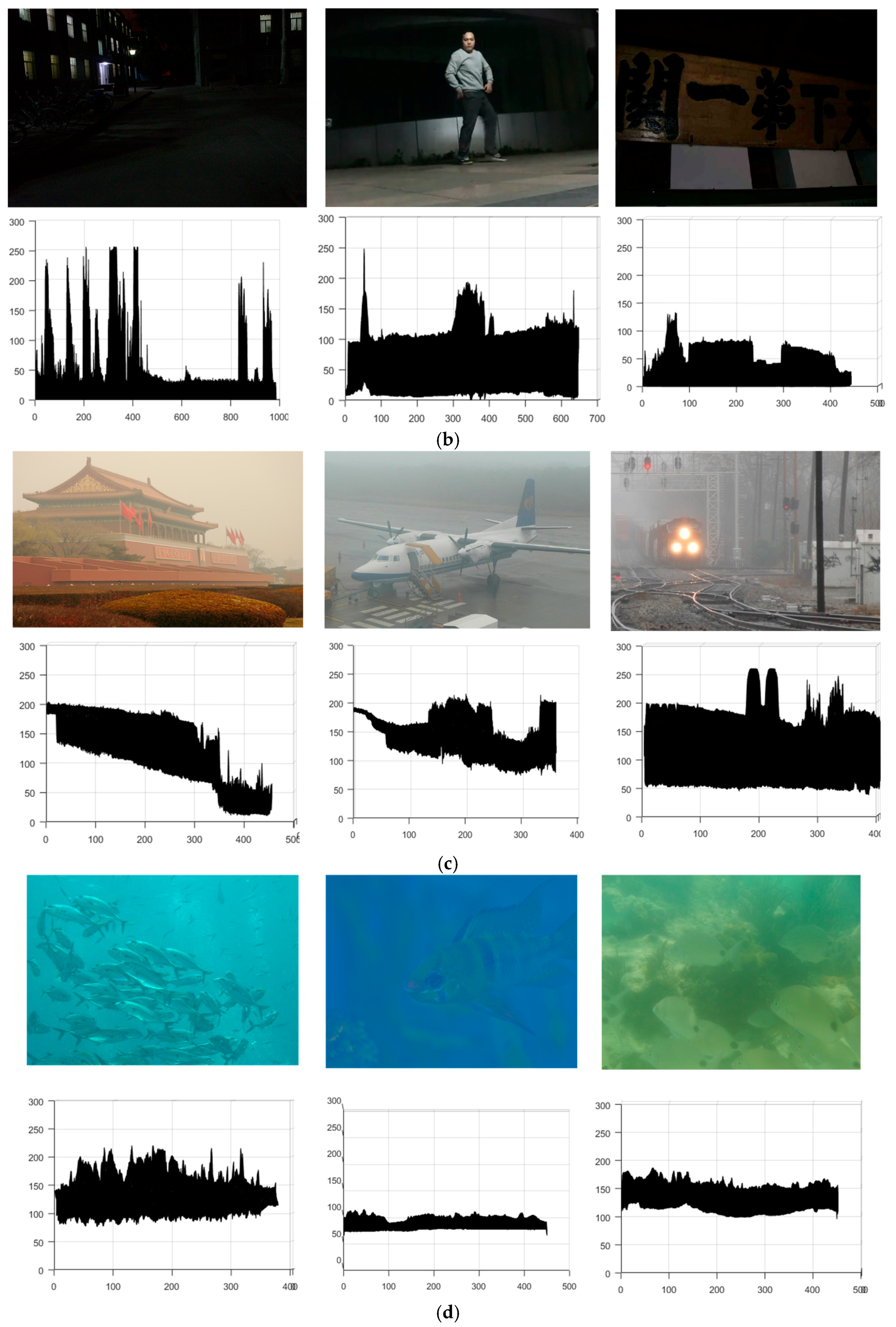
6.2. Scope of Application

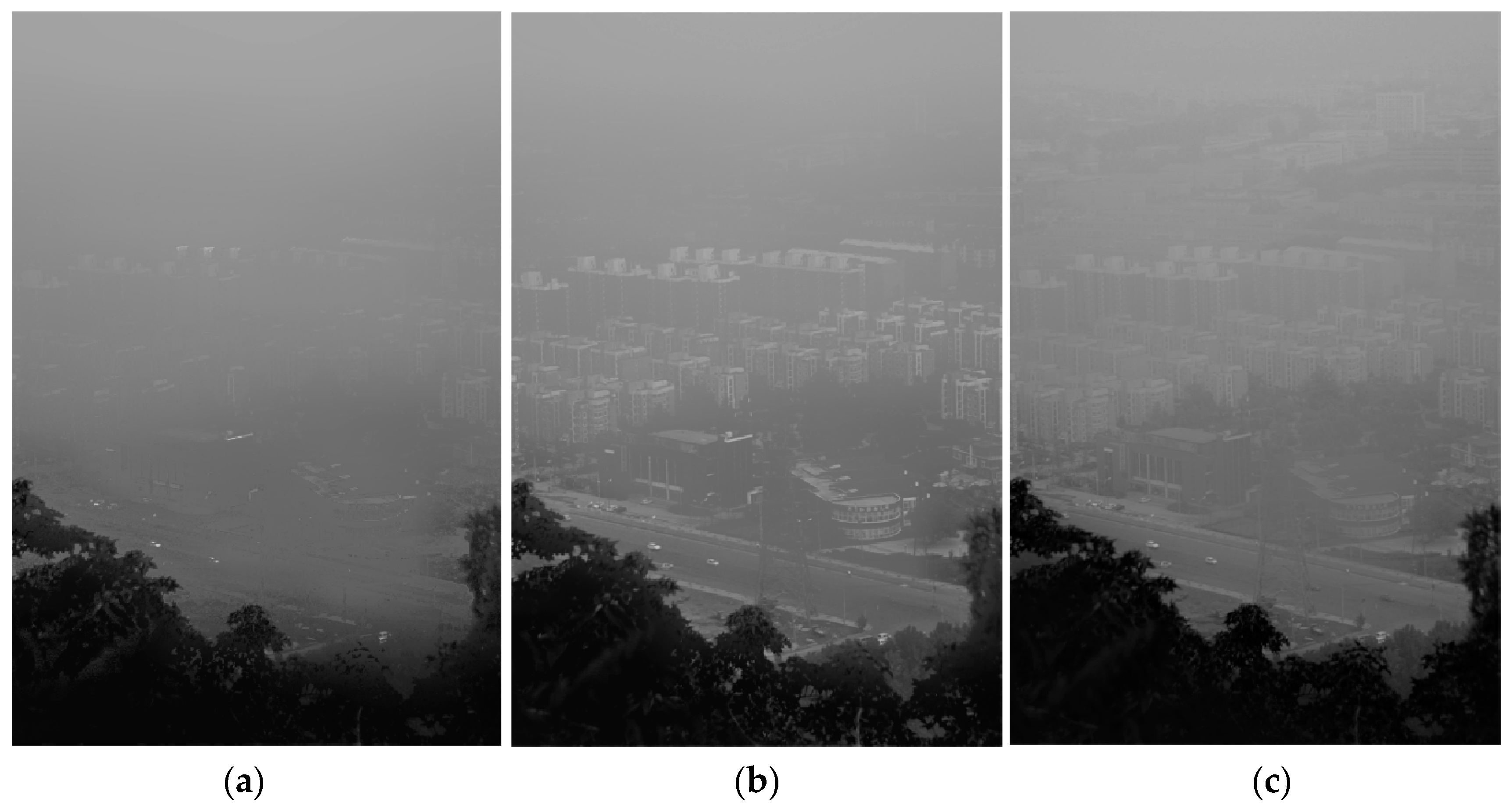
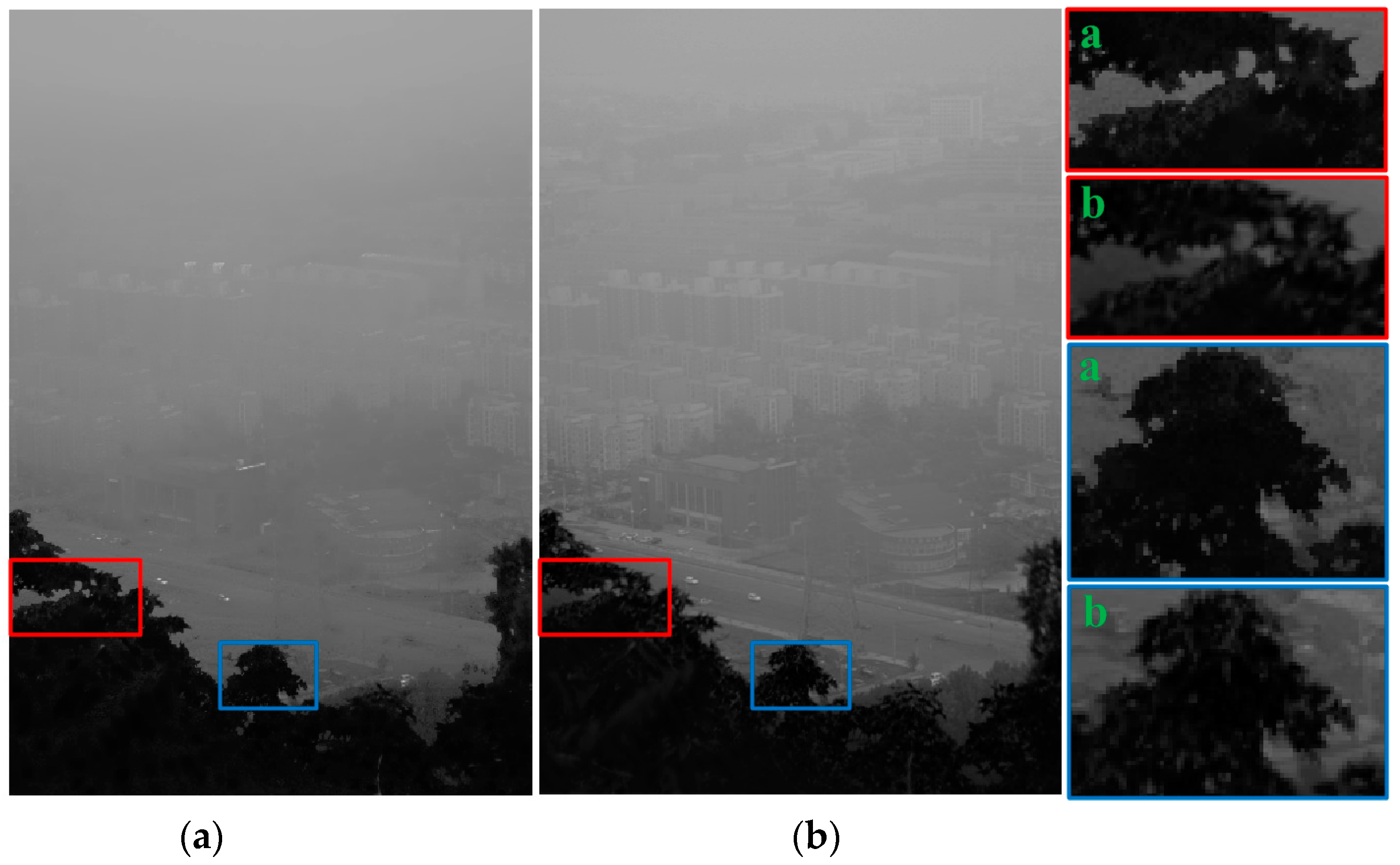
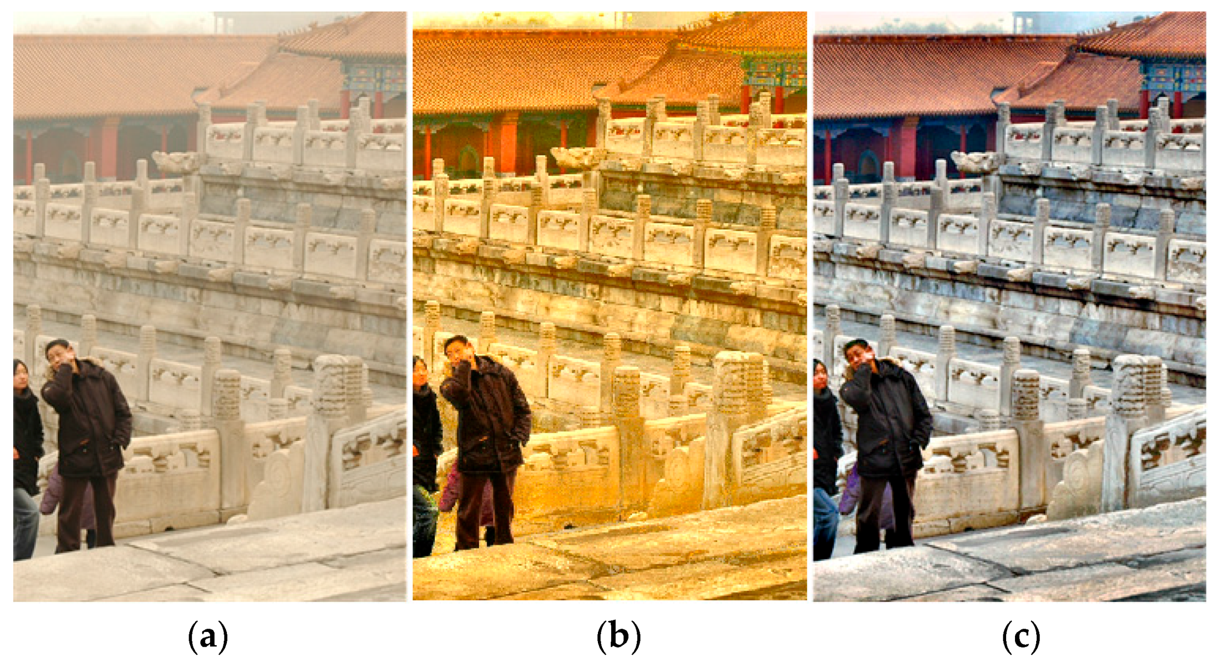
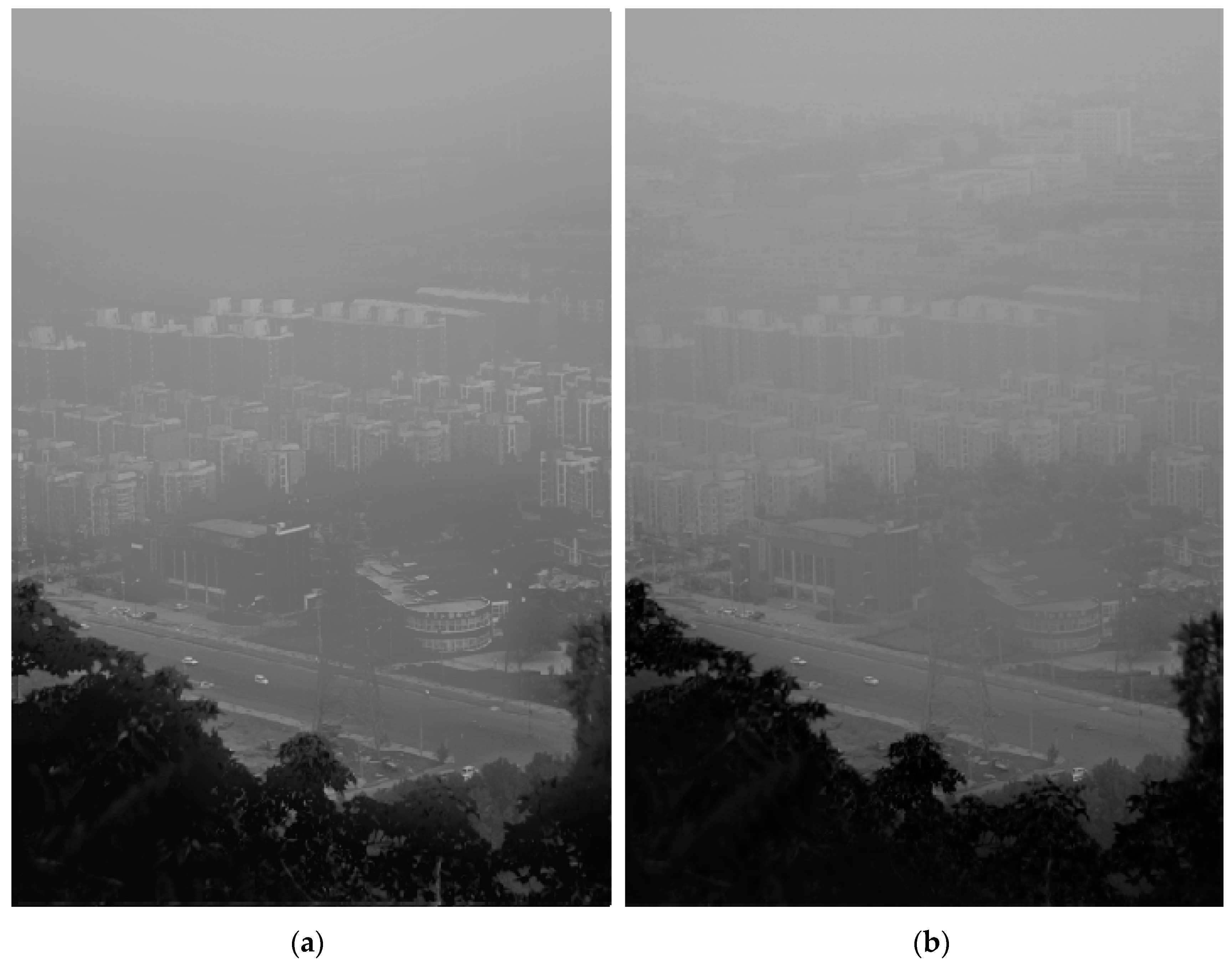
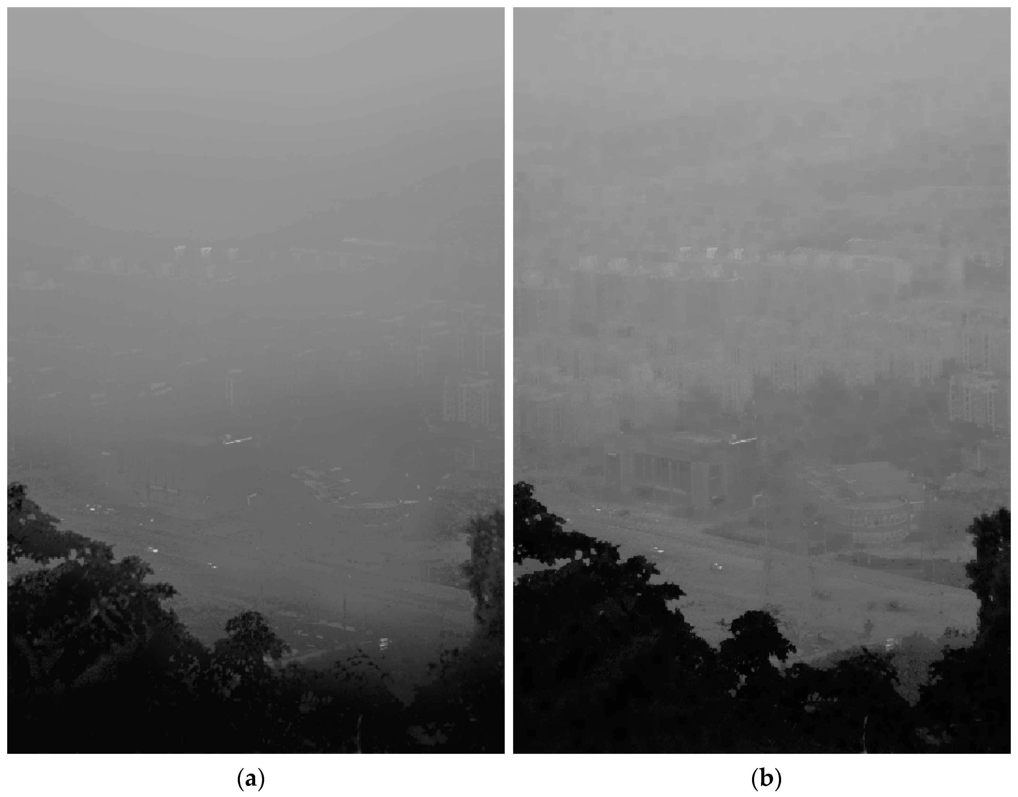
First of all, Figure 10 shows the results of our algorithm for color images including a hazy day, underwater, a nighttime and even a multidegraded image. As can be seen, our approach can stretch the details clearly and recover vivid colors in underwater or heavily hazy regions.

Besides, our approach also works for grayscale images, such as infrared images. According to the different bit depths, we give another set of parameters. Figure 11 shows the video screenshots from a theodolite of the naval base. We stretch the infrared images by a linear model with the max value and min value, which is the most widely used model to display infrared images.

6.3. Haze Removal

Next, we compare our approach with Zhang’s [28], He’s [23], Kim’s [29] and Tan’s [21] approaches for haze removal. In Figure 12, the depth edges between the foreground and background may produce haloes by many dehazing algorithms. As can be seen, the results of other methods usually look dim, and most of them restore the halo, except Zhang’s method. On the contrary, our approach compensates for the illumination and has not introduced any significant haloes.

6.4. Lightning Compensation

We also compare our method with MSR [5], Wang’s [10] and Lin’s [11] approaches for lightning compensation in Figure 13 and Figure 14. Figure 13 shows an image with nonuniform illumination, which has a shadow region. We can see that both MSR and Wang’s approach increase the exposure of the boy inside the tire; however, in some regions there, is an overexposure, such as the letters on the tire.

In contrast, no matter in the shadow regions (boy’s face) or the sunshine regions (tires, boy’s clothing), our approach gives clear details. Figure 14 is a nighttime image, which includes some non-detail information in the dark region. The result of MSR draws out the compressed information, which is regarded as noise. On the other hand, Lin’s result is much better, which increases exposure and suppresses the noise. In this experiment, our approach is similar to Lin’s. Both Lin’s [11] and our approach compensate for the illumination and suppress the useless information in the dark region. Ours restores more details than Lin’s [11], such as the leaves at the top left corner and more textures of the road. However, Lin’s [11] result reduces the glow of light at the side of the road, and has a more comfortable color than ours.

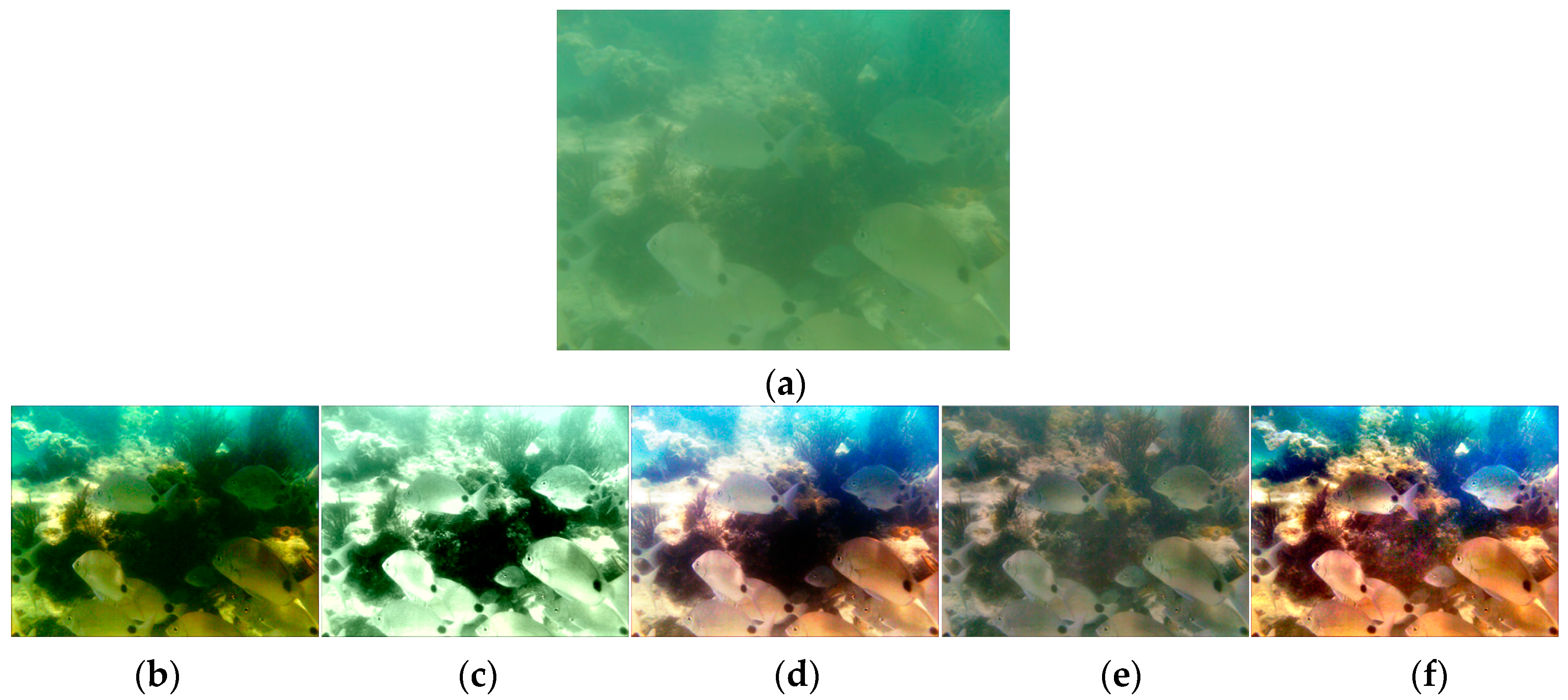
6.5. Underwater Enhancement

Most of the underwater enhancements need a white balancing to discard unwanted color casts, due to various illuminations. In Figure 15, we compare our methods with He et al.’s [23], MSR [5], Ancuti et al.’s [32] and Zhang et al.’s [8] approaches for enhancing the underwater images. It can be seen that He et al.’s approach [23] and MSR [5] have significant contrast stretching of the underwater image, but retain the color casts. Ancuti et al.’s approach [32] applied the gray-world methods for white balancing and restored a comfortable color; however, their results oversaturated the region with brilliant illumination. Zhang et al. proposed an improved MSR to enhance the underwater image and obtained a result with suitable color, but the contrast stretching is very little. Our approach restored a vivid color owing to the gray-world [34]; moreover, there is no oversaturation in our result, and the details of the reef are clearer than other methods.

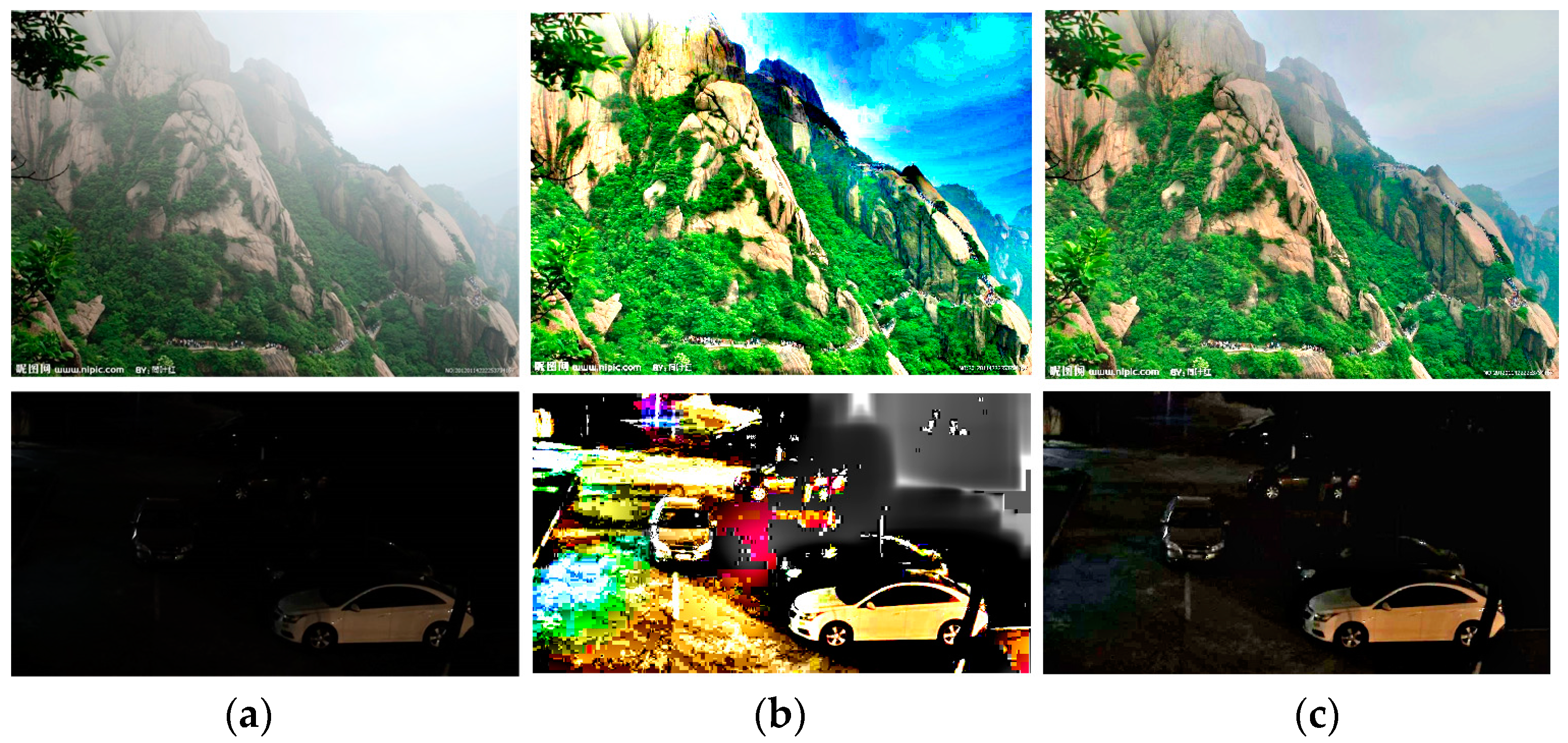
6.6. Multidegraded Enhancement

Figure 16 presents the results of a multiple degraded image, which includes color casts, low illumination and a hazy environment. We compare our results with He et al. [23], Li et al. [30], Lin et al. [11] and Ancuti et al. [32]. As can be seen, all of them can handle a part of the degradation. He et al.’s method removed most of the haze, but kept the red color of the inputs, as well as the restoration looked too dim. Though Li et al.’s algorithm achieved a better result on color recovery, haze removal and illumination compensation, the result still retained the original red hue; Lin et al.’s nighttime enhancement compensated for the low illumination such as the plants in the middle of the road; Ancuti et al.’s result handled all of the degradations, in spite of the overcompensation for illumination, which resulted in a lack of colors (the bushes and leaves are hard to recognize as green).

6.7. Quantitative Comparison

Based on the above results on the multidegraded image in Figure 16, we conducted a quantitative comparison using the MSE (mean squared error) and the SSIM (structural similarity index).

Table 2. Quantitative comparison of Figure 16 based on the MSE and the Structural Similarity index (SSIM).

	He’s [23]	Li’s [30]	Lin’s [11]	Ancuti’s [32]	Avg Changes	Ours
MSE	0.066	0.019	0.023	0.071	0.0283	0.073
SSIM	0.48	0.73	0.88	0.56	−0.4325	0.23

shows the quantitative comparisons, in which the MSE represents the texture details of an image, and the SSIM is used for measuring the similarity between two images.

From Table 2, we can observe that the MSE is inversely proportional to SSIM, meaning that the greater the difference between the results and the input image, the more details are restored. The Avg changes column shows the average changes in MSE and SSIM between the proposed method and those from the other studies. He’s [23] and Ancuti’s [32] approaches had a higher MSE and a lower SSIM than Li’s [30] and Lin’s [11] approaches; in other words, He’s [23] and Ancuti’s [32] approaches were less similar to the input image, as well as restored more details of the image. Our approach had the highest MSE and the lowest SSIM, meaning that the proposed method obtained more texture information than the other methods. From the average changes, we can see that our method improves the MSE and reduces the SSIM more than other methods. That means our approach is better suited for this kind of low contrast images.

7. Conclusions

Image quality can be affected by the shooting of certain scenes, such as hazy, night or underwater, which will degrade the contrast of images. In this paper, we have proposed a generic model for enhancing the low contrast images based on the observation of the 3D surface graph, called the effective space. The effective space is estimated by the dark and bright channel priors, which are patch-based methods. In order to reduce the artifacts produced by the patches, we have also designed the pixel learning for edge-preserving smoothing, which was inspired by online learning. Combining the model with the pixel learning, low contrast image enhancement becomes simpler and has fewer artifacts. Compared with a number of competing methods, our method shows more favorable results. The quantitative assessment demonstrates that our approach can provide an obvious improvement to both traditional and up-to-date algorithms. Our method has been applied to a theodolite of the naval base and can enhance a 720 × 1080 video stream by 20 ms/f (50 fps).

Most of the parameters of our method were set empirically, which depends on some features of an image such as the size or depth. To make a better choice of the parameters, more complex features [36,37,38,39,40] should be studied, which will be figured out systematically in future work. Besides, since the look-up table model replaced the values one by one, the spatial continuity of the image will be destroyed and some noise will be introduced. This is a challenging problem, and an advanced model is needed to keep the memory of spatial continuity. We leave this for future studies.

References

1. Land, E.H. Recent advances in Retinex theory and some implications for cortical computations: Color vision and the natural image. Proc. Natl. Acad. Sci. USA 1983, 80, 5163–5169. [Google Scholar] [CrossRef] [PubMed]
2. Land, E.H. An alternative technique for the computation of the designator in the Retinex theory of color vision. Proc. Natl. Acad. Sci. USA 1986, 83, 3078–3080. [Google Scholar] [CrossRef] [PubMed]
3. Land, E.H. Recent advances in Retinex theory. Vis. Res. 1986, 26, 7–21. [Google Scholar] [CrossRef]
4. Jobson, D.J.; Rahman, Z.; Woodell, G.A. Properties and performance of a center/surround Retinex. IEEE Trans. Image Process. 1997, 6, 451–462. [Google Scholar] [CrossRef] [PubMed]
5. Jobson, D.J.; Rahman, Z.; Woodell, G.A. A multiscale Retinex for bridging the gap between color images and the human observation of scenes. IEEE Trans. Image Process. 1997, 6, 965–976. [Google Scholar] [CrossRef] [PubMed]
6. Kimmel, R.; Elad, M.; Shaked, D.; Keshet, R.; Sobel, I. A Variational Framework for Retinex. Int. J. Comput. Vis. 2003, 52, 7–23. [Google Scholar] [CrossRef]
7. Ma, Z.; Wen, J. Single-scale Retinex sea fog removal algorithm fused the edge information. Jisuanji Fuzhu Sheji Yu Tuxingxue Xuebao J. Comput. Aided Des. Comput. Graph. 2015, 27, 217–225. [Google Scholar]
8. Zhang, S.; Wang, T.; Dong, J.; Yu, H. Underwater Image Enhancement via Extended Multi-Scale Retinex. Neurocomputing 2017, 245, 1–9. [Google Scholar] [CrossRef]
9. Si, L.; Wang, Z.; Xu, R.; Tan, C.; Liu, X.; Xu, J. Image Enhancement for Surveillance Video of Coal Mining Face Based on Single-Scale Retinex Algorithm Combined with Bilateral Filtering. Symmetry 2017, 9, 93. [Google Scholar] [CrossRef]
10. Wang, Y.; Wang, H.; Yin, C.; Dai, M. Biologically inspired image enhancement based on Retinex. Neurocomputing 2016, 177, 373–384. [Google Scholar] [CrossRef]
11. Lin, H.; Shi, Z. Multi-scale retinex improvement for nighttime image enhancement. Opt. Int. J. Light Electron Opt. 2014, 125, 7143–7148. [Google Scholar] [CrossRef]
12. Xie, S.J.; Lu, Y.; Yoon, S.; Yang, J.; Park, D.S. Intensity variation normalization for finger vein recognition using guided filter based singe scale Retinex. Sensors 2015, 15, 17089–17105. [Google Scholar] [CrossRef] [PubMed]
13. Lan, X.; Zuo, Z.; Shen, H.; Zhang, L.; Hu, J. Framelet-based sparse regularization for uneven intensity correction of remote sensing images in a Retinex variational framework. Opt. Int. J. Light Electron Opt. 2016, 127, 1184–1189. [Google Scholar] [CrossRef]
14. Wang, G.; Dong, Q.; Pan, Z.; Zhang, W.; Duan, J.; Bai, L.; Zhanng, J. Retinex theory based active contour model for segmentation of inhomogeneous images. Digit. Signal Process. 2016, 50, 43–50. [Google Scholar] [CrossRef]
15. Jiang, B.; Woodell, G.A.; Jobson, D.J. Novel Multi-Scale Retinex with Color Restoration on Graphics Processing Unit; Springer: New York, NY, USA, 2015. [Google Scholar]
16. Shi, Z.; Zhu, M.; Guo, B.; Zhao, M. A photographic negative imaging inspired method for low illumination night-time image enhancement. Multimedia Tools Appl. 2017, 76, 1–22. [Google Scholar] [CrossRef]
17. Wang, Y.; Zhuo, S.; Tao, D.; Bu, J.; Li, N. Automatic local exposure correction using bright channel prior for under-exposed images. Signal Process. 2013, 93, 3227–3238. [Google Scholar] [CrossRef]
18. Shwartz, S.; Namer, E.; Schechner, Y.Y. Blind Haze Separation. In Proceedings of the IEEE Computer Society Conference on Computer Vision and Pattern Recognition, New York, NY, USA, 17–22 June 2006; pp. 1984–1991. [Google Scholar]
19. Shen, X.; Li, Q.; Tian, Y.; Shen, L. An Uneven Illumination Correction Algorithm for Optical Remote Sensing Images Covered with Thin Clouds. Remote Sens. 2015, 7, 11848–11862. [Google Scholar] [CrossRef]
20. Kopf, J.; Neubert, B.; Chen, B.; Cohen, M.; Cohen, D.; Deussen, O.; Uyttendaele, M.; Lischinski, D. Deep photo: Model-based photograph enhancement and viewing. ACM Trans. Graph. 2008, 27, 1–10. [Google Scholar] [CrossRef]
21. Fattal, R. Single image dehazing. ACM Trans. Graph. 2008, 27, 1–9. [Google Scholar] [CrossRef]
22. Tan, R.T. Visibility in bad weather from a single image. In Proceedings of the IEEE Conference on Computer Vision and Pattern Recognition, CVPR 2008, Anchorage, AK, USA, 23–28 June 2008; pp. 1–8. [Google Scholar]
23. He, K.; Sun, J.; Tang, X. Single Image Haze Removal Using Dark Channel Prior. IEEE Trans. Pattern Anal. Mach. Intell. 2011, 33, 2341–2353. [Google Scholar] [PubMed]
24. He, K.; Sun, J.; Tang, X. Guided Image Filtering. IEEE Trans. Pattern Anal. Mach. Intell. 2013, 35, 1397–1409. [Google Scholar] [CrossRef] [PubMed]
25. Meng, G.; Wang, Y.; Duan, J.; Xiang, S.; Pan, C. Efficient Image Dehazing with Boundary Constraint and Contextual Regularization. In Proceedings of the IEEE International Conference on Computer Vision, Sydney, Australia, 1–8 December 2013; pp. 617–624. [Google Scholar]
26. Jo, S.Y.; Ha, J.; Jeong, H. Single Image Haze Removal Using Single Pixel Approach Based on Dark Channel Prior with Fast Filtering. In Computer Vision and Graphics; Springer: Cham, Switzerland, 2016; pp. 151–162. [Google Scholar]
27. Ju, M.; Zhang, D.; Wang, X. Single image dehazing via an improved atmospheric scattering model. Vis. Comput. 2017, 33, 1613–1625. [Google Scholar] [CrossRef]
28. Zhang, S.; Yao, J. Single Image Dehazing Using Fixed Points and Nearest-Neighbor Regularization. In Proceedings of the Asian Conference on Computer Vision, Taipei, Taiwan, 20–24 November 2016; Springer: Cham, Switzerland, 2016; pp. 18–33. [Google Scholar]
29. Kim, J.-H.; Jang, W.-D.; Sim, J.-Y.; Kim, C.-S. Optimized contrast enhancement for real-time image and video dehazing. J. Vis. Commun. Image Represent. 2013, 24, 410–425. [Google Scholar] [CrossRef]
30. Li, Y.; Tan, R.T.; Brown, M.S. Nighttime Haze Removal with Glow and Multiple Light Colors. In Proceedings of the IEEE International Conference on Computer Vision, Santiago, Chile, 7–13 December 2015; IEEE Computer Society: Washington, DC, USA, 2015; pp. 226–234. [Google Scholar]
31. Ji, T.; Wang, G. An approach to underwater image enhancement based on image structural decomposition. J. Ocean Univ. China 2015, 14, 255–260. [Google Scholar] [CrossRef]
32. Ancuti, C.; Ancuti, C.O.; Haber, T.; Bekaert, P. Enhancing underwater images and videos by fusion. In Proceedings of the 2012 IEEE Conference on Computer Vision and Pattern Recognition, Providence, RI, USA, 16–21 June 2012; pp. 81–88. [Google Scholar]
33. Ma, C.; Ao, J. Red Preserving Algorithm for Underwater Imaging. In Geo-Spatial Knowledge and Intelligence; Springer: Singapore, 2017; pp. 110–116. [Google Scholar]
34. Ebner, M. Color constancy based on local space average color. Mach. Vis. Appl. 2009, 20, 283–301. [Google Scholar] [CrossRef]
35. Van Herk, M. A fast algorithm for local minimum and maximum filters on rectangular and octagonal kernels. Pattern Recognit. Lett. 1992, 13, 517–521. [Google Scholar] [CrossRef]
36. Le, P.Q.; Iliyasu, A.M.; Sanchez, J.A.G.; Hirota, K. Representing Visual Complexity of Images Using a 3D Feature Space Based on Structure, Noise, and Diversity. Lect. Notes Bus. Inf. Process. 2012, 219, 138–151. [Google Scholar] [CrossRef]
37. Gu, K.; Zhai, G.; Lin, W.; Liu, M. The Analysis of Image Contrast: From Quality Assessment to Automatic Enhancement. IEEE Trans. Cybernet. 2017, 46, 284–297. [Google Scholar] [CrossRef] [PubMed]
38. Hou, W.; Gao, X.; Tao, D.; Li, X. Blind image quality assessment via deep learning. IEEE Trans. Neural Netw. Learn. Syst. 2017, 26, 1275–1286. [Google Scholar]
39. Gu, K.; Li, L.; Lu, H.; Lin, W. A Fast Computational Metric for Perceptual Image Quality Assessment. IEEE Trans. Ind. Electron. 2017. [Google Scholar] [CrossRef]
40. Wu, Q.; Li, H.; Meng, F.; Ngan, K.N.; Luo, B.; Huang, C.; Zeng, B. Blind Image Quality Assessment Based on Multichannel Feature Fusion and Label Transfer. IEEE Trans. Circuits Syst. Video Technol. 2016, 26, 425–440. [Google Scholar] [CrossRef]
Figure 1. Images and the projection of their 3D surface graphs on the x-z plane. In the 2D projection, the x-axis is the image width, and the y-axis is the pixel value: (a) the clear images; (b) the low illumination images; (c) the hazy images; (d) the underwater images.
Information 08 00135 g001aInformation 08 00135 g001b
Figure 2. Comparison of α fusion and guided filter: (a) the α fusion, with thred1 = 10, the radius of the mean filter is 40; (b) the guided filter.
Information 08 00135 g002
Figure 3. Comparison of refinement: (a) the pixel learning, with thred1 = 10; (b) the α fusion, with thred1 = 10; (c) the guided filter.
Information 08 00135 g003
Figure 4. Comparison of refinement from different labels: (a) the label is Ibm, with thred1 = 10; (b) the label is Ib, with thred1 = 10.
Information 08 00135 g004
Figure 5. Comparison of refinement: (a) the pixel learning, where thred1 = 10, thred2 = 20; (b) the guided filter.
Information 08 00135 g005
Figure 6. Overenhancement and truncation: (a) the original image; (b) the result without truncation by tD = 255, tU = 0; (c) the result with truncation by tD = 150, tU = 70.
Information 08 00135 g006
Figure 7. Color casts: (a) the original image needs white balance; (b) the result without white balance; (c) the result with white balance.
Information 08 00135 g007
Figure 8. Flow diagram of the proposed algorithm: for the gray scale, brightp and darkp should be skipped, which means the input gray image I = IpU = IpD.
Information 08 00135 g008
Figure 9. Results with different thred1: (a) the original hazy image; (b) thred1 = 1; (c) thred1 = 10; (d) thred1 = 20.
Information 08 00135 g009
Figure 10. Results of enhancement for color images: (a) the original hazy image; (b) our results.
Information 08 00135 g010
Figure 11. Results of enhancement for infrared images (14 bits): thred1 = 800, thred2 = 1600, tD = 4000, tU = 14,000.
Information 08 00135 g011
Figure 12. Comparison of haze removal: (a) input image; and results from using the methods by (b) Zhang’s [28]; (c) He’s [23]; (d) Kim’s [29]; (e) Tan’s [21]; (f) ours; our parameters were set as: for D thred1 = 1, for U thred1 = 20.
Information 08 00135 g012aInformation 08 00135 g012b
Figure 13. Comparison of the nonuniform illumination image: (a) input image; and results from using the methods by (b) multiscale retina-cortex (Retinex) (MSR) [5]; (c) Wang’s [10]; (d) ours.
Information 08 00135 g013
Figure 14. Comparison of the approaches for the nighttime image: (a) input image; and the results from using the methods by (b) MSR [5]; (c) Lin’s [11]; (d) ours.
Information 08 00135 g014
Figure 15. Comparison of the approaches for the underwater image: (a) input image; and the results form using the methods by (b) He’s [23]; (c) MSR [5]; (d) Ancuti’s [32]; (e) Zhang’s [8]; (f) ours.
Information 08 00135 g015
Figure 16. Comparison of the approaches for the underwater image: (a) input image; and the results from using the methods by (b) He’s [23]; (c) Li’s [30]; (d) Lin’s [11]; (e) Ancuti’s [32]; (f) ours.
Information 08 00135 g016