Abstract
There are several methods to forecast precipitation, but none of them is accurate enough since predicting precipitation is very complicated and influenced by many factors. Data assimilation systems (DAS) aim to increase the prediction result by processing data from different sources in a general way, such as a weighted average, but have not been used for precipitation prediction until now. A DAS that makes use of mathematical tools is complex and hard to carry out. In our paper, machine learning techniques are introduced into a precipitation data assimilation system. After summarizing the theoretical construction of this method, we take some practical weather forecasting experiments and the results show that the new system is effective and promising.
1. Introduction
Data assimilation [1,2,3,4,5,6,7,8] is a process by which data from different sources are processed and adjusted in a general or a comprehensive way. In weather forecasting, numerical prediction [9,10,11] models are widely used for predicting future states of the atmosphere. However, these models are dependent on exact initial conditions. The problem is that the real initial conditions of a model are often different from the observation due to the technique or other reasons. Thus, in a narrow way, data assimilation is initially considered to be a process of analyzing and processing the observed data that are conformed to certain spatial and temporal distributions for providing as close to exact initial fields as possible for numerical predictions. This is the narrow way. The main data assimilation methods from the middle of the last century to the present include the function fitting method [12,13] (objective analysis), the stepwise correction method (SCM) [14,15], the optimal interpolation method (OI) [16,17], the variability method (3Dvar, 4Dvar) [18,19], and the ensemble Kalman filtering (EnKF) method [20,21,22]. In these studies, most scientists optimize the initial conditions by constructing a cost function and find the extreme of this cost function [23], finally obtaining optimization by obtaining a, or a set of maximum possible state/s, and we call this the Data Assimilation method. Although there are a lot of data assimilation methods mentioned above, essentially all these methods to solve this problem use statistical and mathematical analysis to find the final solution [24,25]. However, for an effective DAS algorithm, it would be hard to carry out operationally because of the large amount of calculation and some technical problems. For example, the Kalman filtering method does not realize localization in any countries and regions. Later, machine learning methods were introduced into this area, but they are confined to a narrow data assimilation system, in other words, they do not include precipitation, and only basic neural networks were used [26,27,28,29,30].
The main contribution of this paper is to propose a precipitation data assimilation method that makes use of machine learning techniques. In our paper, we use a case-based reasoning system and the precipitation prediction results of numerical models as the inputs for our assimilation system to infer the relationship between the real precipitation value and the predictions. The reason why we introduce case-based reasoning is that its prediction mechanism is different from that of numerical models and the prediction accuracy of these two varies according to the time periods. That is, sometimes the numerical models are better and the other times not. As we know, the main function of a data assimilation system is to output a final prediction that is better than each single one. Thus, data assimilation can output a final precipitation value that is better than both. This would increase the total prediction accuracy. Here, accuracy means the degree to which the result of a measurement, calculation, or specification conforms to a correct value or a standard. In our paper, the accuracy of prediction is valued as MSE (mean squared error): the smaller the MSE, the higher the accuracy. There is another concept called precision compared with accuracy, which means the refinement of a measurement, calculation, or specification, especially as represented by the number of digits given.
Generally speaking, neural networks form the core of a precipitation data assimilation system, setting up the mapping between the inputs and the output without knowing the exact relationship between them. Experiments illustrate that machine learning techniques can better approximate the real precipitation value as much as possible.
The organization of this paper is as follows. In Section 2, we briefly introduce the preliminaries of the paper: data assimilation and neural networks and the case-based reasoning system. Section 3 describes the modeling of a neural network-based data assimilation system. Section 4 describes the experiment to test the system that we propose. Finally, conclusions are given.
2. Preliminaries
2.1. Data Assimilation
In a broad way, data assimilation is a process in which data from different sources are processed and adjusted in a general way and can be used in a comprehensive way. Data assimilation is simply understood with two basic meanings: the first is to combine all kinds of data with different accuracies into an organic one to offer better numerical prediction; the second is to comprehensively use the observation data from different time periods and then to transfer them into corresponding space information.
In a narrow way, data assimilation is considered a process of analyzing and processing the observed data that are conformed to certain spatial and temporal distributions for providing close to exact initial fields of numerical models. The initial states of the numerical model (called analysis) are not determined from the available observations alone. Instead, it is a combination of observation and forecast: observation is the current observation data of the real system and forecast is the prediction that is generated by numerical models propagating information from past observations to the current time. The analysis combines the information in the background (forecast) with that of the current observations, essentially by taking a weighted mean of the two; using estimates of the uncertainty of each to decide their weighting factors. This process is called narrow data assimilation processing. The narrow data assimilation procedure is invariably multivariate and includes approximate relationships between the variables. The observations are of the real system and not of the model’s incomplete representation of that system, and so may have different relationships between the variables from those in the model. To reduce the impact of these problems, incremental analyses are often performed. That is, the analysis procedure determines increments when added to the background to yield the analysis.
The process of creating the analysis in data assimilation often involves minimization of a cost function. A typical cost function would be the sum of the squared deviations of the analysis values from the observations weighted by the accuracy of the observations, plus the sum of the squared deviations of the forecast fields and the analyzed fields weighted by the accuracy of the forecast. This has the effect of making sure that the analysis does not drift too far away from observations and forecasts that are known to usually be reliable. For example,
3D-Var
where B denotes the background error covariance, H is the observational error covariance, x is the initial value, xb is the initial value being added with a perturbation, y is the analysis, R is the observational error covariance and i is the index of time period.
2.2. BP (Back Propagation) Neural Network
The Back Propagation (BP) neural network (shown in Figure 1) includes input layer, hidden layer and output layer and a three-layer structure [11,12,13,14,15] (see Figure 1). The hidden layer can be one or more layers. The basic working principle of a BP network is to input signal Xi through the intermediate node (hidden layer), acting on the output node, after nonlinear transformation to produce the output signal yk. Network training includes input vector X and expected output Y. The error between the value X and the expected output value t is decreased along the gradient direction by adjusting the value of the joint strength wik, between the input node and the hidden layer node and the joint strength vjk between the hidden layer node and the output nodes and the threshold. After several iterations, the weights and threshold are determined corresponding to the minimum error and then the training stops. BP neural network training process consists of two parts: forward propagation and reverse error propagation. Forward transmission occurs, the information from the input layer is processed through the hidden layer and into the output layer, the neurons’ states are only influenced by their previous state. If the desired output is not obtained at the output layer, back propagation is performed and the error signal is returned along the original neuronal connection path. In the process of backwards, the weights of neurons in all layers are modified one by one. This process continues and continues, finally reaching an error signal within the allowable range. In a nutshell, the learning process of the BP network is carried out by multi-layer error correction gradient descent method, which is called the error backward propagation learning algorithm. Error Back Propagation learns the mapping of inputs to outputs, which is done through a process that minimizes the square sum of errors.
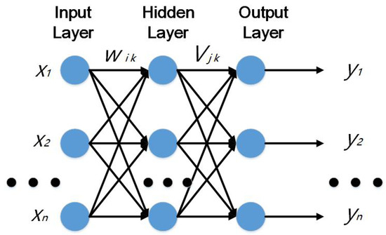
Figure 1.
Back Propagation (BP) neural network basic structure.
When given an input mode X = (x1, x2, …, xm) and a desired mode Y = (y1, y2, …, yn), the actual network output is:
The hidden layer output is:
Network output error square sum:
Among them, wik, vjk respectively denotes weights between the input layer and the hidden layer and the hidden layer to the output layer connection weights; θj, φk respectively represents layer node and the output layer node threshold; m, h, n refers to the input layer, hidden layer, the output layer nodes number. After inputting an input and output and updating the weights and thresholds, it needs to be propagated forward again. When processing one tuple, a method for updating weights and thresholds is called an instance update. Scanning and training all tuples in all training sets is called a cycle. The process of neural network training needs to go through several cycles until the errors fall within a threshold.
2.3. Case-Based Reasoning System
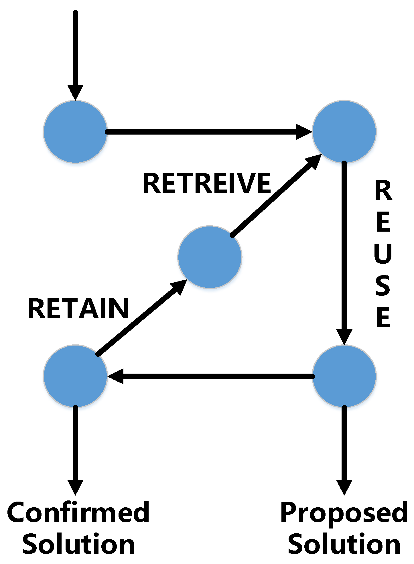
Case-based reasoning (shown in Table 1 and Figure 2) infers new information based on previous experiences. A case is composed of input part X and output part Y.

Table 1.
Values of feature Xi for the example e1 and e2.
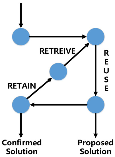
Figure 2.
Case-based learning process.
Case-based reasoning is a method that combines learning with reasoning. A case-based reasoner solves new problems by recording old cases and adapting the most similar one. It interprets new situations by remembering old similar situations and contrasting the new one to the old ones to see which one fits best. After the old cases being properly stored, a new case will enter into the system to get a prediction. The most similar case or cases are chosen, and the prediction of the case is the output of the most similar case. To trigger this method, a distance is required to measure the closeness of two examples. The Euclidean metric can be used as the distance between two objects. Suppose e(Xi) (shown in Table 1) is the value of feature Xi for the example e; (e1(Xi) − e2(Xi)) is the feature difference between example e1 and example e2. One issue is the importance of different features; increasing the weight of one feature increases the importance of this feature. Let wi be the weight of feature Xi. The distance between examples e1 and e2 is then d (e1, e2) = sqrt(∑i wi × (e1(Xi) − e2(Xi))2). In general, the second time solving the problem is easier than the first because we are more competent since we remember our mistakes and therefore can avoid them.
Retrieve: Remembering is the process of retrieving a case or set of cases from memory. In general, it consists of two sub-steps: Recall old cases and Select the best case. The goal of the first step is to retrieve suitable cases that can support the reasoning that occurs in the following step. Good cases are those that have the potential ability to make correct prediction on the new case. Given a new case, we retrieve similar case/cases from the case base, and then select the best subset. This step selects the most promising case/cases to reason with from those generated in the step of Recalling old cases. The purpose of this step is to narrow the set of relevant cases to a few candidates that are worthy of intensive consideration. Sometimes it is proper to choose a best case, and sometimes a small set is needed.
Reuse: Adapt the retrieved case or cases to match with the new case, and propose a solution.
Revise: Evaluate and revise the solution based on how well it works. The revision can involve other reasoning techniques, such as using the proposed solution as a basic point to come up with a more suitable solution, which can be done by a human interactive system.
Retain: Decide whether to keep this new case and its solution in the case base.
3. Description of the Proposed System
The following is the comparison between the previous study and our study towards research objectives. From Figure 3, Figure 4 and Figure 5 we see: (1) A broad assimilation system maps different data from different resources to the real value through mathematical estimation and calculation; (2) A narrow data assimilation system is the same as the broad one, except it only provides as far as exact initial fields for numerical models. The inputs are often composed of observation and forecast. Since the data being assimilated happens before the model processing, it can be understood as “prior”; (3) Our assimilation system aims at precipitation, which has not been covered by previous data assimilation. Since precipitation is a kind of data type that occurs after the numerical processing, it can be understood as “posterior”.
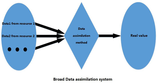
Figure 3.
Broad Data assimilation system.
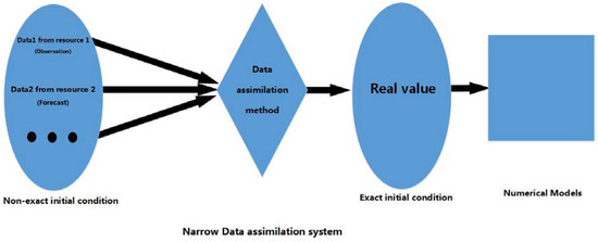
Figure 4.
Narrow (Prior) Data assimilation system.
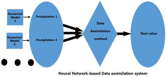
Figure 5.
Posterior Data assimilation system.
A data assimilation system is composed of inputs, the data assimilation method and outputs. In our system, we take the neural network as the core of the data assimilation system. It is an independent data assimilation method itself, not combined with other operational data assimilation methods. However, it could be used as a part of narrow operational data assimilation system. In other words, the data assimilation method can be a mathematical model or a machine learning one (shown in Figure 3, Figure 4 and Figure 5).
What should be noted is that machine learning data assimilation methods and statistical data assimilation methods are very different, although these two are designed to uncover hidden information.
- Machine learning is a data learning algorithm that does not rely on rule design. It can get much information which cannot be described in detail, and the statistical model expresses the relationship between variables in mathematical form.
- The statistical model is based on a series of assumptions but the “nature” does not give any assumptions before it happens. The less the hypothesis of a prediction model, the higher the prediction efficiency can be achieved. Because machine learning does not rely on assumptions about real data, the prediction effect is very good. Statistical models are mathematical reinforcement, dependent on parameter estimation, so need the model builder to know or understand the relationship between variables in advance. For example, the statistical model obtains a simple boundary line in the classification problem, but for complex problems, a statistical model seems to have no way to compare with machine learning algorithms since the machine learning method obtains the information that any boundary cannot be described in detail.
- Machine learning can learn hundreds of or millions of observational samples, prediction and learning synchronization. Some algorithms, such as random forest and gradient boosting, are very fast when dealing with big data. Machine learning deals with data more broadly and deeply. However, statistical models are generally applied to small amounts of data and narrow data attributes. Most commonly this leads to the numerical modeling system alternately performing a numerical forecast and a data analysis. This is known as analysis/forecast cycling. The forecast from the earlier analysis to the current one is often called the background.
The case-based reasoning method is introduced in a broad data assimilation system as a prediction member since the machine learning methods and numerical models have different mechanisms and thus can supplement each other. For example, sometimes the machine learning prediction models are better than numerical prediction models and at other times, the prediction models are better than the machine learning. In whichever situations, the final model will surpass both of them after training properly.
The new system (shown in Figure 6) is composed of several components: Input layer, Prediction layer, Output layer and Final layer.
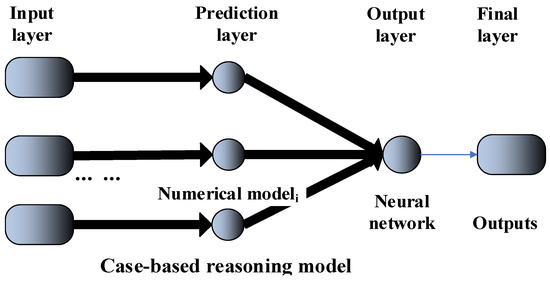
Figure 6.
Neural network-based data assimilation system.
Input layer: the inputs are often a set of samples that could be one dimensional or multidimensional. For a machine learning model, the inputs are usually one dimensional and for numerical models, the inputs are usually multidimensional. In this sense, the inputs of each model do not need to be the same.
Prediction layer: for numerical models, they do not learn before predicting, while for some machine learning models, they have to learn before predicting. But, not all the machine learning methods need to learn before predicting. The models are parallel-arranged and each of them does not rely on the others. In this paper, the models are designed to predict the same variable values. Output layer: this layer outputs the prediction results based on different model types.
Output layer: this layer is the traditional neural network.
Final layer: this layer outputs the final prediction values.
4. Experiments
4.1. Data Formatting
The data in this example is from the Global Ensemble Forecast System (GEFS) of the NCEP (National Centers for Environmental Prediction) data center. GEFS is a global-coverage weather forecast model made up of 21 separate forecasts—or ensemble members—used to quantify the amount of uncertainty in a forecast. GEFS produces output four times a day with weather forecasts for up to 16 days out. The National Centers for Environmental Prediction (NCEP) started the GEFS to address the nature of uncertainty in weather observations, which is used to initialize weather forecast models. The model type is GEFS-MEAN-SPRD but we did not use the SPRD part.
Datasets include real precipitation values and precipitation prediction values from 1 June 2010 to 31 August 2017. This example illustrated how neural networks can be used to approximate the relationship between the real value and the prediction.
4.2. Ranking Key Features
For the case-based reasoning system, we need to appropriately learn how to choose features to predict precipitation. A simple method for searching for a significant feature is to assume that each feature is independent. After testing, we keep temperature, wind, atmosphere pressure and relative humidity as the prediction factors for forecasting precipitation.
For the neural network-based data assimilation system, we set the GEFS (global ensemble forecasting system) precipitation average and the case-based reasoning system precipitation prediction as the inputs, and the real precipitation as the output. The training samples are composed of inputs and output.
Besides, we need to guarantee that the produced mapping is not over-fitted. In our example, inputs are the predictive precipitation values from different resources and the target outputs are the corresponding real values of the precipitation.
5. Discussion
Once some significant features have been identified, we can use this information to approximate the real atmospheric conditions. Because the neural network is started with random weights, the results of the neural network after training vary slightly each time although the examples or the training set is the same. To avoid this randomness, the random seed is set to reproduce the same results every time.
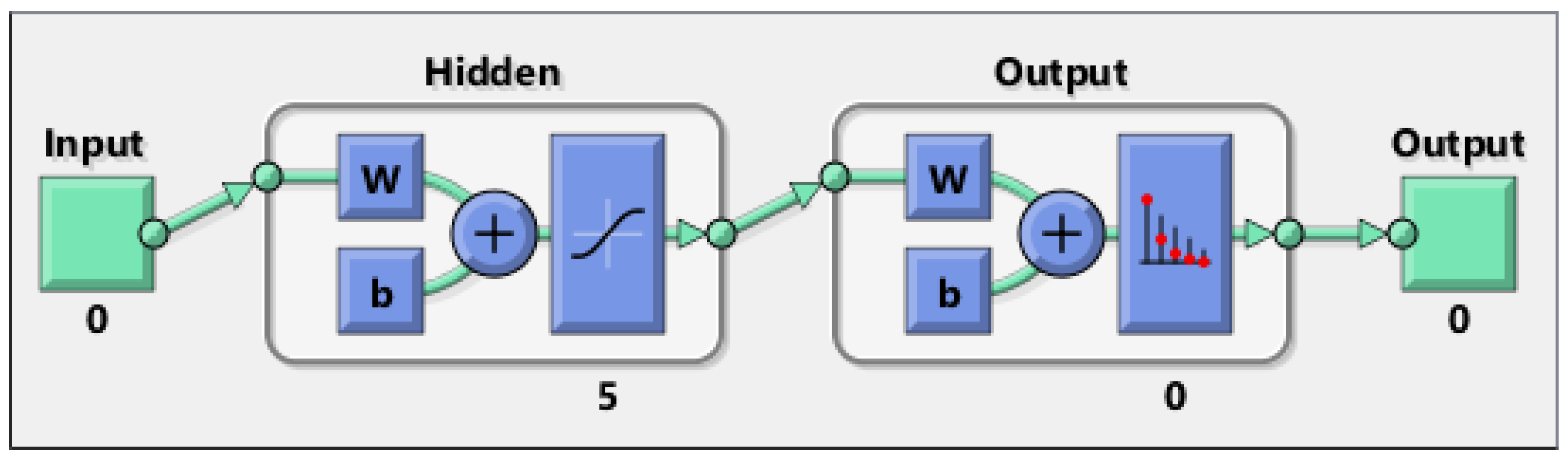
A one-hidden layer feed forward neural network with 5 hidden layer neurons is created and trained and is shown in Figure 7. The samples are automatically divided into training, validation and test sets. The training set is used to train the neural network. Training continues and continues until it achieves the desired performance on the validation set. The test set provides a completely independent measure of network accuracy. Both the input and output at the stage of creating the neural network have sizes of 0 because the network has not yet been configured to match our input and target data. This will change when the network begins its training process.
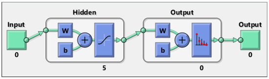
Figure 7.
Neural network created.
Now the network is ready to be trained. The samples are automatically separated into a training set, a validation set and a test set. The training set is used to teach the network. The training process continues and continues until the neural network achieves improvement on the validation set. The test set provides a completely independent measure of network accuracy. The neural network Training Tool displays the NN being trained and the algorithms being used during training. It also shows that the changing training state in the training process and the stopped training criteria that are highlighted in green. All these processes use the command line shown in below:
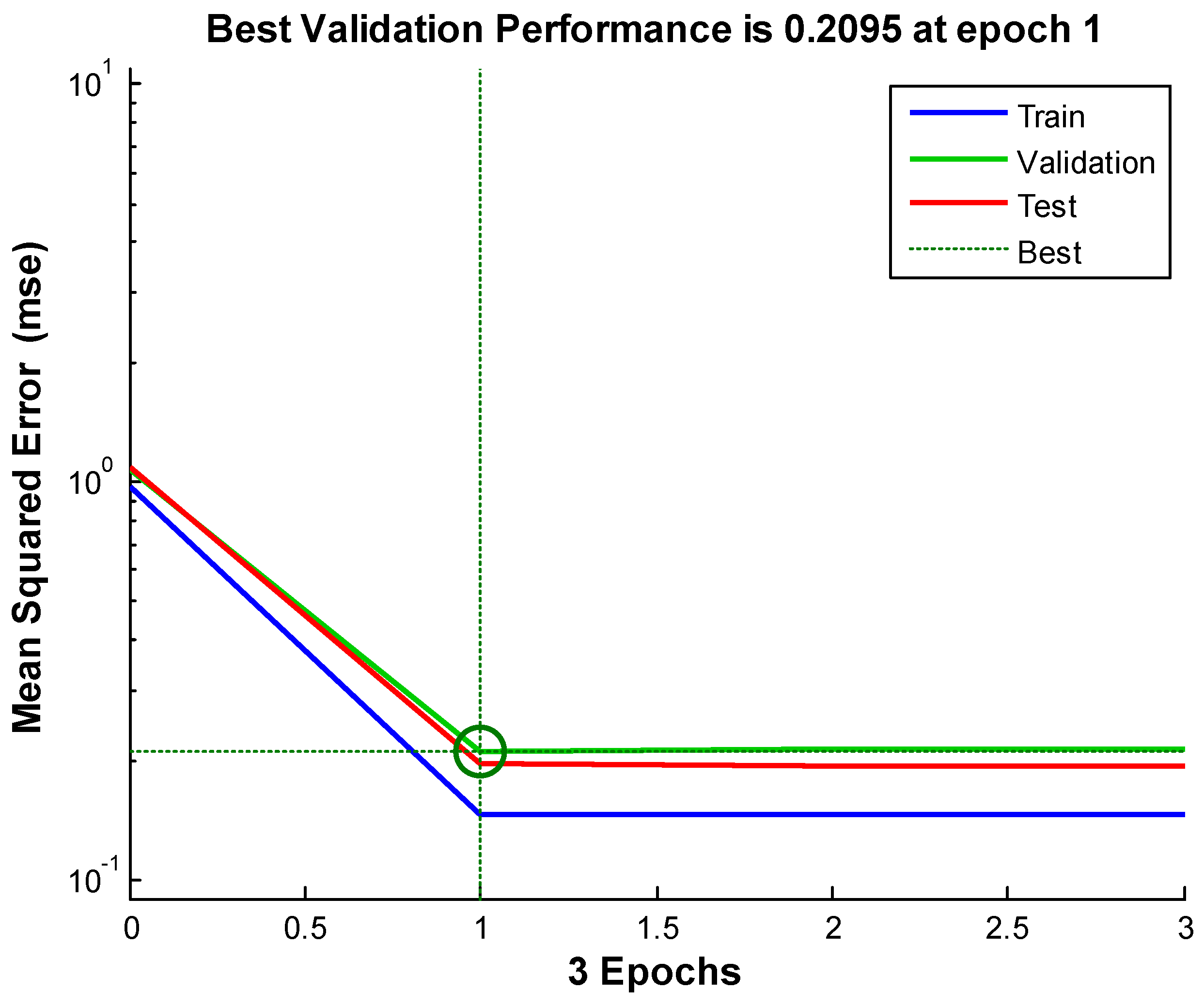
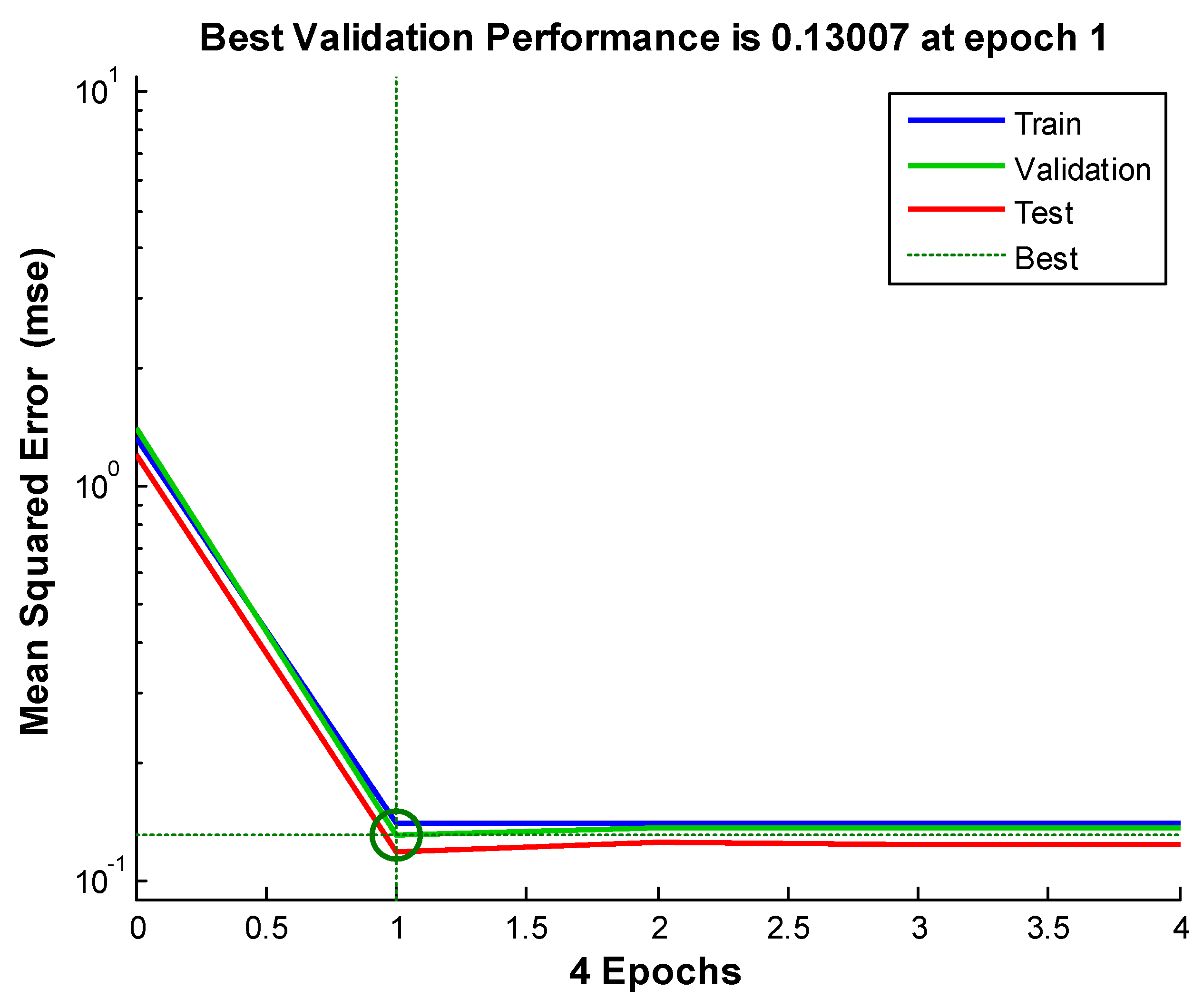
Figure 8, Figure 9 and Figure 10 shows the neural network’s performances improved during training. Performance is measured in terms of mean squared error, and shown in log scale. It rapidly decreased as the network was trained. Performance is shown for each of the training, validation and test sets. The version of the network that did best on the validation set after training.
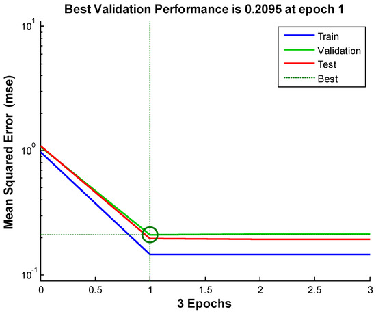
Figure 8.
Neural network-based data assimilation result for station 1.
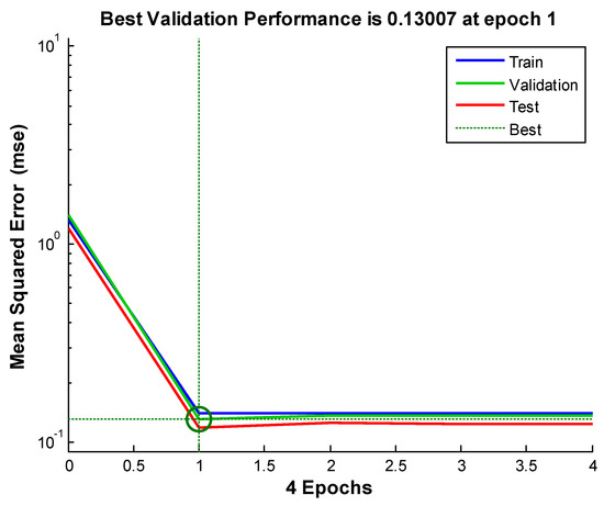
Figure 9.
Neural network-based data assimilation result for station 2.
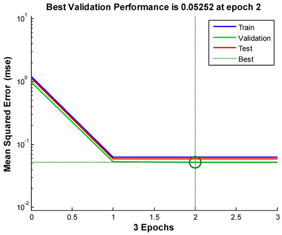
Figure 10.
Neural network-based data assimilation result for station 3.
We see from the Figures and the tables below (Table 2): the neural network-based data assimilation results for stations 1 to 3 share the same characteristics. That is: the errors of our neural network-based data assimilation system are smaller than the ensemble average and the case-based reasoning. Comparing to the previously tried method, the neural network is progress.
Table 2.
Neural network-based data assimilation results.
The trained neural network can now be tested with the testing samples we partitioned from the main dataset. The testing data was not used in training in any way and hence provides an “out-of-sample” dataset to test the network on. This will give us a sense of how well the network will do when tested with data from the real world. The figures below show that the testing result is not over-fitted. Here, “Epoch” means iterative training of a neural network. An Epoch is a single pass through the entire training set, followed by testing of the verification set.
Generally speaking, the experiments show that the accuracy of our system is pretty good, which is very promising.
6. Conclusions
A broad assimilation system approximates the relationship between the real value and the analysis. A narrow data assimilation system is a sort of broad assimilation system but only provides as far as exact initial fields for numerical models. Since the data being assimilated in a narrow system comes before the model processing, it can be understood as “prior”. In our paper, we propose a precipitation data assimilation system, which has not been covered by previous data assimilation systems. Since precipitation is a kind of data type that occurs after the numerical processing, it can be understood as “posterior”.
In our system, the case-based reasoning system and the numerical models’ precipitation prediction results are set as the inputs to our assimilation system in order to infer the relationship between the real precipitation value and the predictions. The case-based reasoning method and the numerical models have different prediction mechanisms and thus can supplement each other. For example, sometimes the machine learning prediction models are better than the numerical prediction models and at other times, the numerical prediction models are better than the machine learning. In whatever situations, the final model will surpass both of them after training properly. The neural networks form the core of the precipitation data assimilation system, setting up the mapping between the inputs and the output without knowing the exact relationship between them. The experiments illustrate that our system can increase precipitation prediction accuracy.
Author Contributions
J.L. conceived the study. J.L. conducted the experiments and analyzed the results. J.L. and W.H. and X.Z. wrote the manuscript and edited and revised the manuscript.
Acknowledgments
This work was supported by the Shanxi scholarship council of China (No. 2015-121).
Conflicts of Interest
The authors declare no conflict of interest.
References
- Carton, J.A.; Giese, B.S. A Reanalysis of Ocean Climate Using Simple Ocean Data Assimilation (SODA). Mon. Weather Rev. 2008, 136, 2999–3017. [Google Scholar] [CrossRef]
- Williams, M.; Schwarz, P.A.; Law, B.E. An improved analysis of forest carbon dynamics using data assimilation. Glob. Chang. Biol. 2010, 11, 89–105. [Google Scholar]
- Fossum, K.; Mannseth, T. Parameter sampling capabilities of sequential and simultaneous data assimilation: II. Statistical analysis of numerical results. Inverse Probl. 2014, 30, 114003. [Google Scholar] [CrossRef]
- Dee, D.P.; Uppala, S.M.; Simmons, A.J. The ERA-Interim reanalysis: Configuration and performance of the data assimilation system. Q. J. R. Meteorol. Soc. 2011, 137, 553–597. [Google Scholar] [CrossRef]
- Makarynskyy, O.; Makarynska, D.; Rusu, E. Filling gaps in wave records with artificial neural networks. In Maritime Transportation and Exploitation of Ocean and Coastal Resources; Taylor & Francis Group: London, UK, 2005; Volume 2, pp. 1085–1091. [Google Scholar]
- Butunoiu, D.; Rusu, E. Wave modeling with data assimilation to support the navigation in the Black Sea close to the Romanian Ports. In Proceedings of the Second International Conference on Traffic and Transport Engineering (ICTTE), Belgrade, Serbia, 27–28 November 2014. [Google Scholar]
- Butunoiu, D.; Rusu, E. A data assimilation scheme to improve the Wave Predictions in the Black Sea. In Proceedings of the OCEANS 2015, Genoa, Italy, 18–21 May 2015; pp. 1–6. [Google Scholar]
- Rusu, E.; Raileanu, A. A multi-parameter data-assimilation approach for wave prediction in coastal areas. J. Oper. Oceanogr. 2016, 9, 13–25. [Google Scholar] [CrossRef]
- Leith, C.E. Numerical weather prediction. Rev. Geophys. 1975, 13, 681–684. [Google Scholar] [CrossRef]
- Buizza, R.; Tribbia, J.; Molteni, F. Computation of optimal unstable structures for a numerical weather prediction model. Tellus 2010, 45, 388–407. [Google Scholar]
- Rusu, L.; Soares, C.G. Impact of assimilating altimeter data on wave predictions in the western Iberian coast. Ocean Model. 2015, 96, 126–135. [Google Scholar] [CrossRef]
- Lorenz, E.N. Energy and Numerical Weather Prediction. Tellus 2010, 12, 364–373. [Google Scholar]
- Rodwell, M.J.; Palmer, T.N. Using numerical weather prediction to assess climate models. Q. J. R. Meteorol. Soc. 2010, 133, 129–146. [Google Scholar] [CrossRef]
- Kug, J.S.; Lee, J.Y.; Kang, I.S. Systematic Error Correction of Dynamical Seasonal Prediction of Sea Surface Temperature Using a Stepwise Pattern Project Method. Mon. Weather Rev. 2010, 136, 3501–3512. [Google Scholar] [CrossRef]
- Ghil, M.; Malanotte-Rizzoli, P. Data Assimilation in Meteorology and Oceanography. Adv. Geophys. 1991, 33, 141–266. [Google Scholar]
- Tombette, M.; Mallet, V.; Sportisse, B. PM10 data assimilation over Europe with the optimal interpolation method. Atmos. Chem. Phys. 2009, 9, 57–70. [Google Scholar] [CrossRef]
- Lee, E.H.; Jong, C. PM10 data assimilation over south Korea to Asian dust forecasting model with the optimal interpolation method. Asia-Pac. J. Atmos. Sci. 2013, 49, 73–85. [Google Scholar] [CrossRef]
- Piccolo, C.; Cullen, M. Adaptive mesh method in the Met Office variational data assimilation system. Q. J. R. Meteorol. Soc. 2011, 137, 631–640. [Google Scholar] [CrossRef]
- Krysta, M.; Blayo, E.; Cosme, E. A Consistent Hybrid Variational-Smoothing Data Assimilation Method: Application to a Simple Shallow-Water Model of the Turbulent Midlatitude Ocean. Mon. Weather Rev. 2011, 139, 3333–3347. [Google Scholar] [CrossRef]
- Wu, C.C.; Lien, G.Y.; Chen, J.H. Assimilation of Tropical Cyclone Track and Structure Based on the Ensemble Kalman Filter (EnKF). J. Atmos. Sci. 2010, 67, 3806–3822. [Google Scholar] [CrossRef]
- Wu, C.C.; Huang, Y.H.; Lien, G.Y. Concentric Eyewall Formation in Typhoon Sinlaku (2008). Part I: Assimilation of T-PARC Data Based on the Ensemble Kalman Filter (EnKF). Mon. Weather Rev. 2012, 140, 506–527. [Google Scholar] [CrossRef]
- Almeida, S.; Rusu, L.; Guedes Soares, C. Application of the Ensemble Kalman Filter to a high-resolution wave forecasting model for wave height forecast in coastal areas. In Maritime Technology and Engineering; Taylor & Francis Group: London, UK, 2015; pp. 1349–1354. [Google Scholar]
- Torn, R.D. Performance of a Mesoscale Ensemble Kalman Filter (EnKF) during the NOAA. High-Resolution Hurricane Test. Mon. Weather Rev. 2010, 138, 4375–4392. [Google Scholar] [CrossRef]
- Skachko, S.; Errera, Q.; Ménard, R. Comparison of the ensemble Kalman filter and 4D-Var assimilation methods using a stratospheric tracer transport model. Geosci. Model Dev. 2014, 7, 1451–1465. [Google Scholar] [CrossRef]
- Tong, J.; Hu, B.X.; Huang, H. Application of a data assimilation method via an ensemble Kalman filter to reactive urea hydrolysis transport modeling. Stoch. Environ. Res. Risk Assess. 2013, 28, 729–741. [Google Scholar] [CrossRef]
- Härter, F.P.; de Campos Velho, H.F.; Rempel, E.L. Neural networks in auroral data assimilation. J. Atmos. Sol.-Terr. Phys. 2008, 70, 1243–1250. [Google Scholar] [CrossRef]
- Cintra, R.S.; Haroldo, F.C.V. Data Assimilation by Artificial Neural Networks for an Atmospheric General Circulation Model. In Advanced Applications for Artificial Neural Networks; InTech: London, UK, 2018. [Google Scholar]
- Pereira, H.F.; Haroldo, F.C.V. Multilayer perceptron neural network in a data assimilation scenario. Eng. Appl. Comput. Fluid Mech. 2010, 4, 237–245. [Google Scholar] [CrossRef]
- Santhosh, B.S.; Shereef, I.K. An efficient weather forecasting system using artificial neural network. Int. J. Environ. Sci. Dev. 2010, 1, 321–326. [Google Scholar]
- Rosangela, C.; Haroldo, C.V.; Steven, C. Tracking the model: Data assimilation by artificial neural network. In Proceedings of the 2016 International Joint Conference on Neural Networks (IJCNN), Vancouver, BC, Canada, 24–29 July 2016; pp. 403–410. [Google Scholar]


© 2018 by the authors. Licensee MDPI, Basel, Switzerland. This article is an open access article distributed under the terms and conditions of the Creative Commons Attribution (CC BY) license (http://creativecommons.org/licenses/by/4.0/).