


Analytical and Numerical Investigation of Two-Dimensional Heat Transfer with Periodic Boundary Conditions

1
Department of Mathematics, Kocaeli University, TR-41380 Kocaeli, Türkiye
2
Department of Mechanical Engineering, Kocaeli University, TR-41380 Kocaeli, Türkiye
*
Author to whom correspondence should be addressed.
Computation 2024, 12(1), 11; https://doi.org/10.3390/computation12010011
Submission received: 8 November 2023
/
Revised: 7 December 2023
/
Accepted: 2 January 2024
/
Published: 10 January 2024
(This article belongs to the Special Issue 10th Anniversary of Computation—Computational Heat and Mass Transfer (ICCHMT 2023))
Abstract
:A two-dimensional heat diffusion problem with a heat source that is a quasilinear parabolic problem is examined analytically and numerically. Periodic boundary conditions are employed. As the problem is nonlinear, Picard’s successive approximation theorem is utilized. We demonstrate the existence, uniqueness, and constant dependence of the solution on the data using the generalized Fourier method under specific conditions of natural regularity and consistency imposed on the input data. For the numerical solution, an implicit finite difference scheme is used. The results obtained from the analytical and numerical solutions closely match each other.
1. Introduction
The investigation of a mathematical model has broad implications for a great number of important applications, such as chemical diffusions [1,2], heat conduction problems, [3,4,5], population dynamics [6], thermoelasticity [7], medical science, electrochemistry [8], engineering, and control theory. This necessitates the analysis of two-dimensional parabolic partial differential equations with nonlocal boundary conditions [9,10,11].
The heat diffusion equation is one of the two-dimensional quasilinear parabolic problems. It is employed to determine temperature distribution in every region of the domain at desired time for conduction heat transfer problems. Heat transfer by conduction involves temperature differences in a solid or stationary fluid. Information on temperature distribution in a solid can be utilized to determine structural integrity through assessing thermal stresses, expansions, deflections, and cracks. The evaluation and propagation of granite thermal stresses and thermal cracks with time are shown in Figure 1 [12]. The temperature distribution can also be used to optimize the thickness of an insulating material or to determine the compatibility of the material with special coatings or adhesives used [13].
Initial and boundary conditions are required for solving the two-dimensional quasilinear parabolic problem, such as the heat diffusion equation. Some of boundary conditions for the heat diffusion equation, Dirichlet (or first kind) determines the fixed temperature at surfaces. For example, the surface is very close to this when it comes into contact with a melting solid and/or a boiling liquid. In both cases, heat transfer occurs at the surface, whereas the surfaces remain at the temperature of phase-changing process [13]. Neumann (or the second type) corresponds to the presence of constant heat flux on the surface. This heat flux is related to the temperature at the surface according to Fourier’s law and can be accomplished by bonding a thin electric heater to the surface. A special case of this situation corresponds to a perfectly insulated or adiabatic surface. A periodic boundary condition is combined with Dirichlet and Neumann boundary conditions [14], and it is set to isolate repeating temperature distribution in the solution’s domain [15].
The periodic boundary condition, a special case of the nonlocal boundary [16] condition, is used in the present investigation. Generally, the periodic boundary condition is often employed in numerical simulations and mathematical models. Additionally, the periodic boundary condition results from many important applications in heat transfer, fluid dynamics, life sciences, and used lunar theory [14,17,18].
There are analytical methods available for solving two-dimensional quasilinear parabolic problems. One of these methods is the Fourier method. Baglan and Kanca analytically solved the two-dimensional quasilinear parabolic problem (heat diffusion) with an inverse coefficient and a heat source using the Fourier method [14,19]. The two-dimensional heat diffusion equation with time-dependent thermal conductivity and a heat source problem is analytically solved with the Fourier method by the same authors [20]. Additionally, similar analytical solutions for fractional diffusion equations can be found in the literature [21,22,23].
In order to solve the two-dimensional quasilinear parabolic problem, several numerical methods are available, such as the finite difference method [24,25], the finite element method [26,27], the finite volume method [28], and the lattice Boltzmann methods [15,29,30]. Denghan solved the one-dimensional heat diffusion equation numerically using the finite difference method [31]. In this study, three different schemes were employed, namely, the backward time-centered space (BTCS) implicit scheme, the implicit Crandall’s method, the forward time-centered space (FTCS) explicit scheme, and the Dufort–Frankel three-level techniques. The Crank–Nicolson implicit scheme is used to numerically solve the one-dimensional heat diffusion equation with an inverse coefficient by Baglan et al. [32]. Kanca and Baglan numerically solved the two-dimensional heat diffusion equation with periodic boundary conditions [20]. An implicit finite difference scheme is used for numerical solutions. Hamila et al. [33] investigated the effects of changes in thermal conductivity on several transient heat transfer problems using the lattice Boltzmann methods (LBM). Benchmark problems containing conduction and/or radiation with constant thermal conductivity were calculated and simulated. The heat diffusion equation was solved numerically by exclusively using the lattice Boltzmann methods. The numerical results closely aligned with the available results in the literature.
The finite difference method is one of the existing numerical methods considered in the present investigation that can be applied to solve partial differential equations. The finite difference method is based on the discretization of differential equations through finite difference equations. Finite difference approximations have algebraic forms and relate the value of a dependent variable at one point in the solution region to the values at some neighboring points. Using Taylor series is the most usual way to construct these approximations. The numerical method recommended here is the implicit finite difference method. This method supports second order accuracy in the spatial grid sizes and first order time grid size. The explicit finite scheme has a restriction of determining time step size due to stability requirements for the numerical solution of the two-dimensional heat diffusion equation.
In the present paper, we establish the existence, uniqueness, and continuous dependence of the solution on the data. We derive the analytical solution by the Fourier Method and Picard’s successive approximation for the two-dimensional heat diffusion problem with periodic boundary conditions [14,19,20]. For the numerical solution, we employ an implicit finite difference approximation. The numerical solution demonstrates good agreement with the analytical solution.
This problem is nonlinear. Obtaining an analytical solution for a nonlinear problem is only possible through a few methods, namely, the Fourier Method, the maximum principle method, and/or the operation method. The periodic boundary condition used in the problem poses a challenging condition, and analytically solving this boundary condition is very difficult. Generally, in the literature, there are very few analytical solutions for problems that are both nonlinear and have periodic boundary conditions. As mentioned before, we utilized the Fourier method along with the Picard’s successive approximation for our analytical solution. We compared this analytical solution with a numerical solution, highlighting the novelty of our study.
2. The Problem with Periodic Boundary Conditions
Let us examine the two-dimensional, quasilinear heat diffusion problem with the heat source given below,
with the initial condition,
and with the periodic boundary conditions,
Studies involving equations similar to the heat diffusion equation we solved in our work can be found in the literature [13,14,19,20,32]. In Equations (1)–(4), where is temperature distribution, h is a source function, and represent the direction, and and are time and maximum time, respectively. The domain size is for the and directions. is the initial condition. A schematic figure of the problem with boundary conditions is shown in Figure 2.
where the Fourier coefficients:
Then, we obtain the solution:
where , , , , and are the Fourier coefficients of the source function.
3. Analytical Solution of the Problem
Let us assume the following rules for the functions used in the problem:
- (A)
Let L be constant,
- (B)
- Let have the following properties:
Definition 1.
is called Banach (B) norm.
Problem (1)–(4) is a nonlinear problem; therefore, an iterative method should be employed to determine the existence, uniqueness, and convergence of the problem. The solution using the Picard Successive Iteration method is as follows.
Theorem 1.
Let the assumptions (A)–(B) be satisfied, then the problem has a unique solution.
Proof.
As an iteration for the problem.
where N is the iteration number.
By applying the Cauchy, Bessel, and Hölder inequalities and the Lipschitz condition, we have
where , , , , and are the Fourier coefficients of the source function. M presents the arbitrary constant.
From the theorem, .
Applying for the step ,
We receive since .
Let us show that is converged for .
By applying the Cauchy, Bessel, and Hölder inequalities and the Lipschitz condition, we have
where let .
Applying for the step N,
We obtain .
Let us show that is converged for .
By applying the Cauchy, Bessel, and Hölder inequalities and the Lipschitz condition, we have
From the Gronwall’s inequality,
From Equation (12), we receive .
To show the uniqueness, we receive two solutions for the problem .
By applying the Cauchy, Bessel, and Hölder inequalities and the Lipschitz condition, we have
From the Gronwall’s inequality,
We receive . □
4. Stability of Solution
Theorem 2.
Let the assumptions (A)–(B) be satisfied. Then, the problem is constantly dependent on the data.
Proof.
By applying the Cauchy, Bessel, and Hölder inequalities and the Lipschitz condition, we have
From the Gronwall’s inequality,
From Equation (14), . Then, . □
5. Numerical Method for Problem
The analytical solution described above, which involves Fourier series, is itself an approximate solution. To validate this approximate solution using another approximate method, namely, the numerical method, we performed a numerical solution following the analytical solution.
In this section, we use an implicit finite difference approximation [14,27,28] of the discretized problems (1)–(4);
where the computational domain is discretized as follows:
, , , , , and .
Where , , and are the space α direction, space β direction, and time steps, respectively. nx, ny, and n are three positive integers.
, and .
In order to define periodic boundary conditions (Equations (17) and (18)) for the implicit finite difference scheme, a one-dimensional schematic figure with numerical meshes is represented in Figure 3. Point-1 and point-nα are the boundary points of the one-dimensional solution domain. When determining spatial discretization with a finite difference scheme, the used finite difference formulations are defined as
where , and the coefficient matrix can be rewritten for one-dimensional solution domain.
This one-dimensional formulation and coefficient matrix can be extended to a two-dimensional solution domain. A two-dimensional schematic figure with numerical meshes (9 finite difference meshes) is represented in Figure 4. Of course, a matrix is constructed for 9 finite difference meshes; therefore, the matrix size is 9 × 9. Point-1, -2, and -3 are periodic with Point-7, -8, and -9, respectively, in the β-direction. Point-1, -4, and -7 are periodic with -3, -6, and -9, respectively, at the α direction. The coefficient matrix can be written as
where . If a large number of meshes are used, the matrix can be extended in a same way. For example, if we have 20 meshes in both the α and β directions, our matrix size will be 400 × 400, the total number of elements in the matrix is 160,000, and our matrix can be constructed in the same manner to define points of periodic boundary conditions and points of inner (no periodic boundary condition points).
The methods that are described above were implemented in-house using finite difference code via the FORTRAN Programming language. The obtained results were visualized using the program Tecplot 360 [34].
Example 1.
Consider the heat diffusion problem with heat sources (1)–(4):
The temperature distribution is given as
with the heat source,
and with the initial condition,
We determined the time step size to be . The discretization of spaces or mesh sizes in the α and β directions are considered equal (). To determine mesh sizes in the α and β directions, a grid independence study was conducted. For the grid-independence study, fifteen different grid resolutions are used.
In the α and β directions, the same numbers of grid were used because of the equal grid size () being considered. In Figure 5, two different grid resolutions are illustrated among fifteen different resolutions. The displayed grid numbers are 2500 and 6400. For every grid resolution, we observed an area-weighted averaged value of temperature for the whole solution domain. Figure 6 shows the grid-independent study of area-weighted averaged value of temperature. According to Figure 6, the mesh number of 6400 is taken as the grid independent mesh number. In this case, eighty grids are used for the α and β directions; therefore, our mesh size for the α and β directions is obtained as 0.03926875 m.
Figure 7 shows the (a) exact and (b) numerical solutions for the temperature with the time at 0.1 s. The exact and numerical solutions are paraboloidal. Maximum and minimum temperature values are observed at corners and at the middle of the solution domain, respectively. Due to periodic boundary conditions at the side of solution domain, temperatures are the same at the side of the solution domain. Also, the exact and numerical solutions are quite similar.
Figure 8 depicts the (a) absolute error and (b) relative absolute error for the temperature with the time at 0.1 s. Absolute error is defined as the absolute value of the difference between the exact solution value and the numerical solution. According to Figure 7a, the maximum absolute error is observed at center of the solution domain, and the absolute error is higher at the corners of the solution domain. At the center of the solution domain, an approximate absolute error of 0.1 is observed. The relative absolute error is the ratio of the absolute error to the exact solution. The magnitude of the absolute error in terms of the exact solution is determined using the relative absolute error. Similar to the absolute error, the maximum relative error, which is 0.03, is observed at the center of the solution domain. At the corners of the solution domain, the relative absolute error is in the order of 0.01. As time progresses, the absolute error and relative absolute error remain in the same order, and these errors are reasonable.
Figure 9 presents the numerical predictions of the temperature distributions at the times (a) 0.1 s, (b) 0.25 s, and (c) 0.5 s. As one can see, the temperature distributions at these specific times are paraboloid. The concavity of the paraboloid increases with time. The minimum and the maximum values of the temperature appear at the center and corners of the solution domain, respectively, at all times.
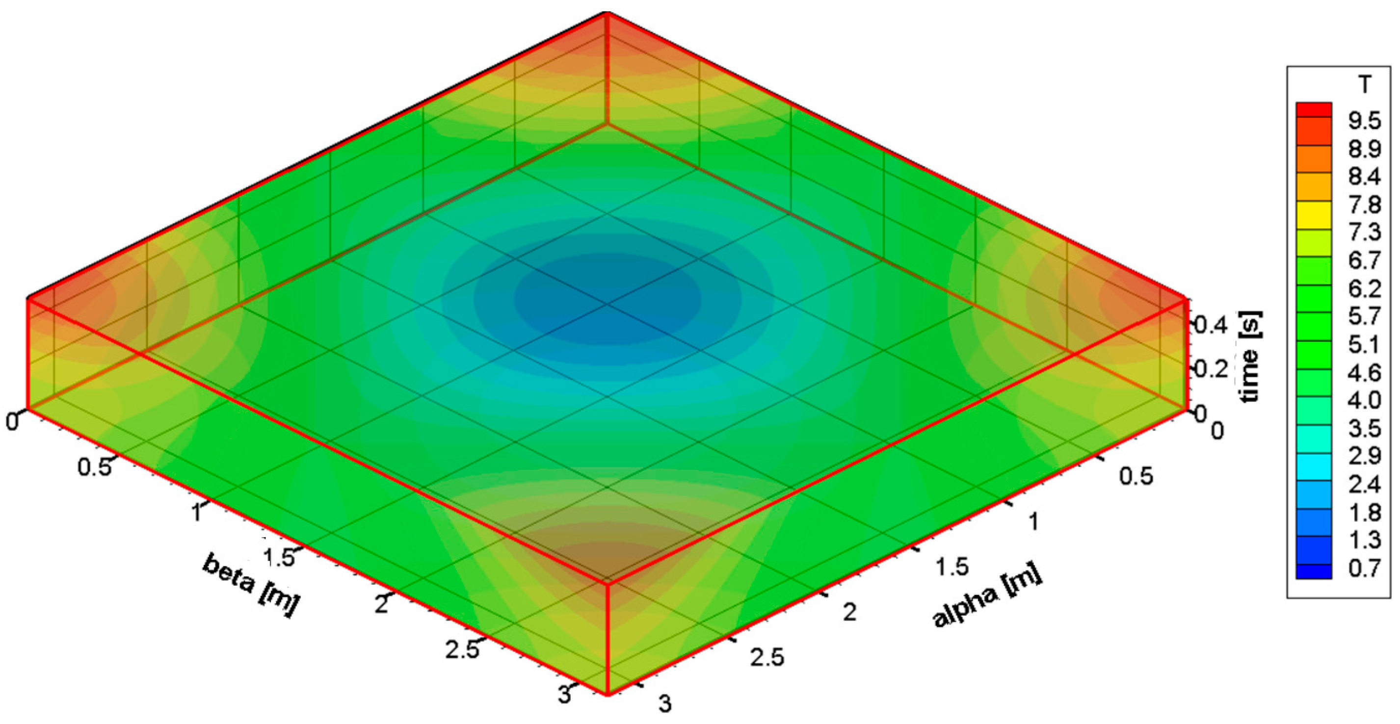
In order to visualize all time intervals in a single figure, Figure 10 illustrates the temperature distribution over a time range from 0 s to 0.5 s. Paraboloids are not shown in this representation. Maximum and minimum temperature values are observed at the corners and center of the solution domain, respectively, at all times. Additionally, with increasing time, the temperature values of the corners increase, and the temperature values of the centers decrease.
Fundamentally, this study has focused on the analytical and numerical solution of a two-dimensional, time-dependent system with heat generation. However, it has not extensively delved into the specific applications of this problem. Nevertheless, the results obtained from this problem could be applied in a suitable context by other researchers.
6. Limitations and Future Scope
This problem is characterized by specific limits and assumptions, constituting a time-dependent, two-dimensional heat diffusion problem with a heat source and periodic boundary conditions. Due to the applied periodic boundary conditions, temperature distributions at the edges and corners of the solution domain are found to be identical. In systems with heat generation, the temperature profile at a specific time tends to exhibit a parabolic shape. As time progresses, the slope of this parabolic nature also increases.
For future studies, this problem can be expanded into three dimensions, enabling an investigation into the influence of the third dimension on heat diffusion. As an analytical solution method, the maximum principle and/or the operation method may be considered in future work. For numerical solutions, various schemes can be employed in the finite difference method, or alternative methods such as the finite volume method and the lattice Boltzmann methods could be explored.
7. Conclusions
An analytical and numerical investigation of a two-dimensional heat diffusion problem with a heat source has been conducted. This problem is a quasi-linear parabolic problem, and we used an initial condition and a periodic boundary condition to determine the temperature in the solution domain. Due to the problem being nonlinear, Picard’s successive approximation theorem is used. Under certain conditions of natural regularity and consistency imposed upon the input data, we establish the existence, uniqueness, and constant dependence of the solution on the data using the generalized Fourier method. An implicit finite difference scheme is employed for the numerical solution. The number of numerical meshes, where results do not change, is determined according to the grid independence study. In light of the analytical and numerical solution, the distribution of the temperature forms a paraboloid at a certain time. With increasing time, the concavity of the parabola increases. At the time of 0.1 s, the maximum absolute error and relative error occur in the middle of the solution domain at 0.1 and 0.03, respectively. Therefore, we can conclude that the analytical solution and numerical solutions are closely aligned. Also, with increasing time, the degrees of absolute and relative absolute remain the same. For future studies, extending the problem to three dimensions can investigate the influence of the third dimension on heat diffusion. Analytically, considering the maximum principle and/or the operation method is an option. Numerically, exploring various schemes in the finite difference method or alternative methods, such as finite volume and the lattice Boltzmann methods, is possible.
Author Contributions
Conceptualization, İ.B. and E.A.; methodology, İ.B.; software, E.A.; validation, E.A; formal analysis, İ.B.; investigation, İ.B. and E.A.; resources, İ.B.; data curation, E.A.; writing—original draft preparation, E.A.; writing—review and editing, İ.B. and E.A.; visualization, E.A.; supervision, İ.B.; All authors have read and agreed to the published version of the manuscript.
Funding
This research received no external funding.
Data Availability Statement
Data are contained with this article.
Conflicts of Interest
The authors declare no conflicts of interest.
Nomenclature
| is the initial temperature. | |
| are the Fourier coefficients of initial condition. | |
| is the temperature distribution. | |
| is a source function. | |
| are the Fourier coefficients of source function. | |
| are the Fourier coefficients. | |
| is an arbitrary constant. | |
| is a Lipschitz coefficient. | |
| is a converged space. | |
| is an iterative number. |
References
- Permikin, D.V.; Zverev, V.S. Mathematical model on surface reaction diffusion in the presence of chemical reaction. Int. J. Heat Mass Transf. 2013, 57, 215–221. [Google Scholar] [CrossRef]
- Tredenick, E.C.; Farewell, T.W.; Forster, W.A. Modeling of diffusion of a hydrophilic ionic fertilizer in plant cuticles: Surfactant and hygroscopic effects. Front. Plant Sci. 2018, 9, 1888. [Google Scholar] [CrossRef] [PubMed]
- Canon, J.R. The solution of the heat equation subject to the specification of energy. Q. Appl. Math. 1963, 21, 155–160. [Google Scholar] [CrossRef]
- Canon, J.R. Determination of an unknown heat source from overspecified boundary data. SIAM J. Numer. Anal. 1968, 5, 275–286. [Google Scholar] [CrossRef]
- Zhu, Q.; Tran, H.; Yang, H. Heat conduction: Mathematical modeling and experimental data. J. Emerg. Investig. 2021, 4, 1–4. [Google Scholar] [CrossRef] [PubMed]
- Venkatesha, P.; Eunice, G.B.; Akshaya, B.; Arya Kumari, S. Mathematical modeling of population growth. Int. J. Sci. Eng. Manag. 2017, 2, 117–121. [Google Scholar]
- Avey, M.; Fantuzzi, N.; Sofiyev, A. Mathematical modeling and analytical solution of thermoelectric stability problem of functionally graded nanocomposite cylinders within different theories. Mathematics 2022, 10, 1081. [Google Scholar] [CrossRef]
- Turnbull, A.; Ferriss, D.H. Mathematical modelling of the electrochemistry in corrosion fatigue cracks in structural steel cathodically protected in sea water. Corros. Sci. 1986, 26, 601–628. [Google Scholar] [CrossRef]
- Dehghan, M. Implicit locally one-dimensional methods for two-dimensional diffusion with a non-local boundary condition. Math. Comput. Simul. 1999, 49, 331–349. [Google Scholar] [CrossRef]
- Siddique, M. Solving two-dimensional diffusion equations with nonlocal boundary conditions by a special class of Padé approximants. Syst. Cybern. Inform. 2010, 8, 23–29. [Google Scholar]
- Mohebbi, A. A numerical algorithm for determination of a control parameter in two-dimensional parabolic inverse problems. Acta Math. Appl. Sin. Engl. Ser. 2015, 31, 213–224. [Google Scholar] [CrossRef]
- Li, Q.; Yin, T.; Li, X.; Shu, R. Experimental and numerical investigation on thermal damage of granite subjected to heating and cooling. Mathematics 2021, 9, 3027. [Google Scholar] [CrossRef]
- Bergmann, T.L.; Lavine, A.S.; Incropera, F.P.; Dewitt, D.P. Fundamentals of Heat and Mass Transfer, 7th ed.; John Wiley & Sons: Danver, MA, USA, 2011. [Google Scholar]
- Baglan, I.; Kanca, F. Two-dimensional inverse quasilinear parabolic problems with periodic boundary conditions. Appl. Anal. 2019, 98, 1549–1565. [Google Scholar] [CrossRef]
- Mohamad, A.A. Lattice Boltzmann Method Fundamentals and Engineering Applications with Computer Codes, 2nd ed.; Springer: London, UK, 2019. [Google Scholar]
- Afshar, S.; Soltanalizadeh, B. Solution of the two-dimensional second-order diffusion equation with nonlocal boundary conditions. Int. J. Pure Appl. Math. 2014, 94, 119–131. [Google Scholar] [CrossRef]
- Rao, Y.; Zhang, Y.; Xu, Y.; Ke, H. Experimental study and numerical analysis of heat transfer enhancement and turbulent flow over shallowly dimples channel surfaces. Int. J. Heat Mass Transf. 2020, 160, 120195. [Google Scholar] [CrossRef]
- Hill, G.W. On the part of the motion of the lunar perigee which is a function of the mean motions of the sun and moon. Acta Math 1886, 8, 1–36. [Google Scholar] [CrossRef]
- Kanca, F.; Baglan, I. Solution of the boundary-value problem of heat conduction with parabolic conditions. Ukr. Math. J. 2020, 72, 232–245. [Google Scholar] [CrossRef]
- Kanca, F.; Baglan, I. Analysis for two-dimensional inverse quasilinear parabolic problem by Fourier Method. Inverse Probl. Sci. Eng. 2021, 29, 1912–1945. [Google Scholar] [CrossRef]
- Yasmin, H.; Aljahdaly, N.F.; Saeed, A.M.; Shah, R. Probing families of optical soliton solutions in fractional perturbed Radhakrishnan-Kundu-Lakshmanan model with improved versions of extended direct algebraic method. Fractal Fract. 2023, 7, 512. [Google Scholar] [CrossRef]
- Yasmin, H.; Aljahdaly, N.F.; Saeed, A.M.; Shah, R. Investigating families of solution solutions for the complex structured coupled fractional Biswas-Arshed model in Birefringent fibers using a novel analytical technique. Fractal Fract. 2023, 7, 491. [Google Scholar] [CrossRef]
- Yasmin, H.; Aljahdaly, N.F.; Saeed, A.M.; Shah, R. Investigating symmetric soliton solutions for the fractional coupled Konno-Onno system using improved versions of a novel analytical technique. Mathematics 2023, 11, 2686. [Google Scholar] [CrossRef]
- Morton, K.W.; Mayers, D.F. Numerical Solution of Partial Differential Equation, 2nd ed.; Cambridge University Press: Cambridge, UK, 2005. [Google Scholar]
- Dmitriev, V.G.; Danilin, A.N.; Popova, A.R.; Pshenichnova, N.V. Numerical analysis of deformation characteristics of elastic inhomogeneous rotational shells at arbitrary displacements and rotating angles. Computation 2022, 10, 184. [Google Scholar] [CrossRef]
- Benim, A.C.; Zinser, W. Investigation into finite element analysis of confined turbulent flows using a k-ε model of turbulence. Compt. Methods Appl. Mech. Eng. 1985, 51, 507–523. [Google Scholar] [CrossRef]
- Benim, A.C. Finite element analysis of confined turbulent swirling flows. Int. J. Num. Meth. Fluids 1990, 11, 697–717. [Google Scholar] [CrossRef]
- Versteeg, H.K.; Malalasekera, W. An Introduction to Computational Fluid Dynamics, 2nd ed.; Pearson, Prentice Hall: London, UK, 2007. [Google Scholar]
- Chen, S.; Doolen, G.D. Lattice Boltzmann method for fluid flows. Annu. Rev. Fluid Mech. 1998, 30, 329–364. [Google Scholar] [CrossRef]
- Succi, S. The Lattice Boltzmann Equation for Fluid Dynamics and Beyond; Oxford University Press: Oxford, UK, 2001. [Google Scholar]
- Denghan, M. Efficient techniques for the second-order parabolic equation subject to nonlocal specifications. Appl. Num. Math. 2005, 12, 39–62. [Google Scholar] [CrossRef]
- Baglan, I.; Kanca, F.; Mishra, V.N. Determination of an unknown heat source from integral overdetermination condition. Iran J. Sci. Technol. Trans. Sci. 2018, 42, 1373–1382. [Google Scholar] [CrossRef]
- Hamila, R.; Chaabane, R.; Askri, F.; Jemni, A.; Nasrallah, S.B. Lattice Boltzmann method for heat transfer problems with variable thermal conductivity. Int. J. Heat Technol. 2017, 35, 313–324. [Google Scholar] [CrossRef]
- Tecplot Inc. Tecplot 360 2008 Release 1; Tecplot Inc.: Bellevue, WA, USA, 2007. [Google Scholar]
Figure 1.
Evaluation and propagation of granite thermal stress field and thermal cracks [12].
Figure 1.
Evaluation and propagation of granite thermal stress field and thermal cracks [12].
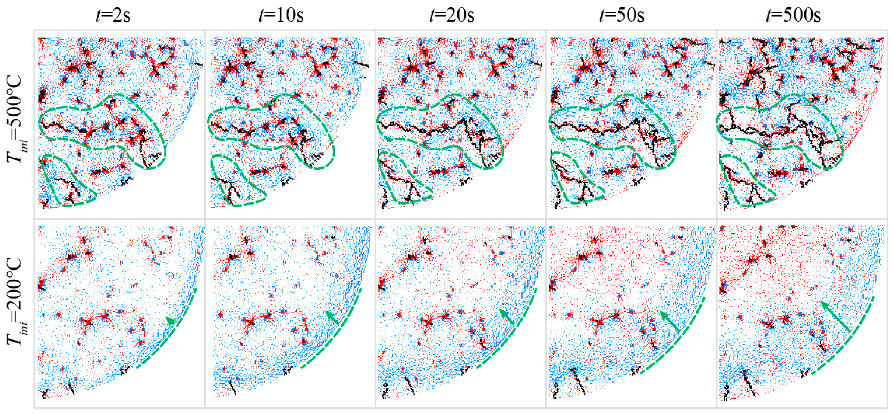
Figure 2.
Schematic figure of the problem with boundary conditions.

Figure 3.
One-dimensional schematic figure with numerical meshes.

Figure 4.
Two-dimensional schematic figure with numerical meshes.
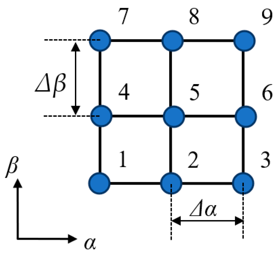
Figure 5.
Two different grid resolutions.
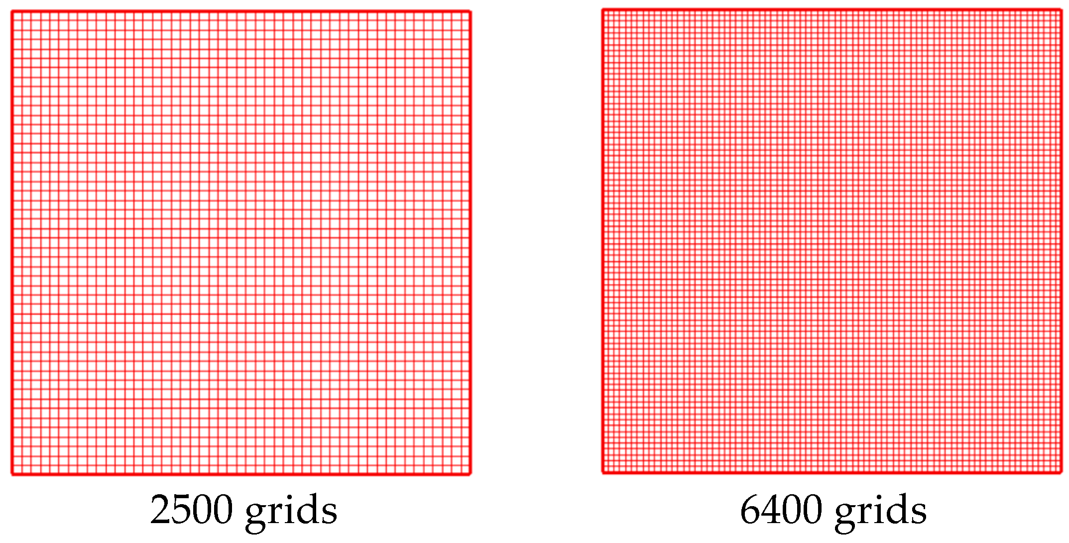
Figure 6.
Grid independence study of area-weighted averaged value of temperature.

Figure 7.
The (a) exact and (b) numerical solutions for T(α, β, 0.1 s).
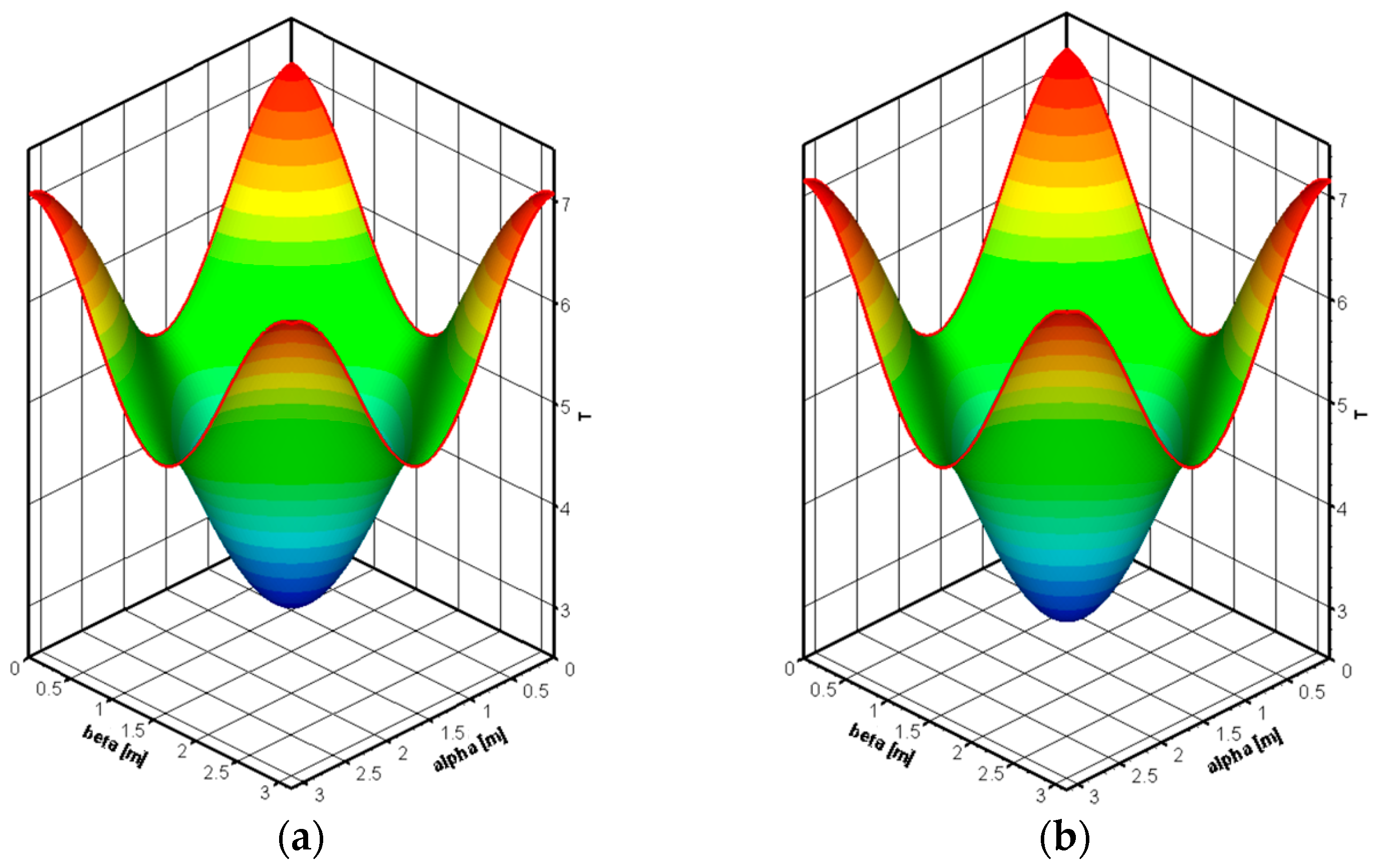
Figure 8.
The (a) absolute error and (b) relative absolute error of T(α, β, 0.1 s).

Figure 9.
Numerical predictions of T distributions at times (a) 0.1 s, (b) 0.25 s, and (c) 0.5 s.
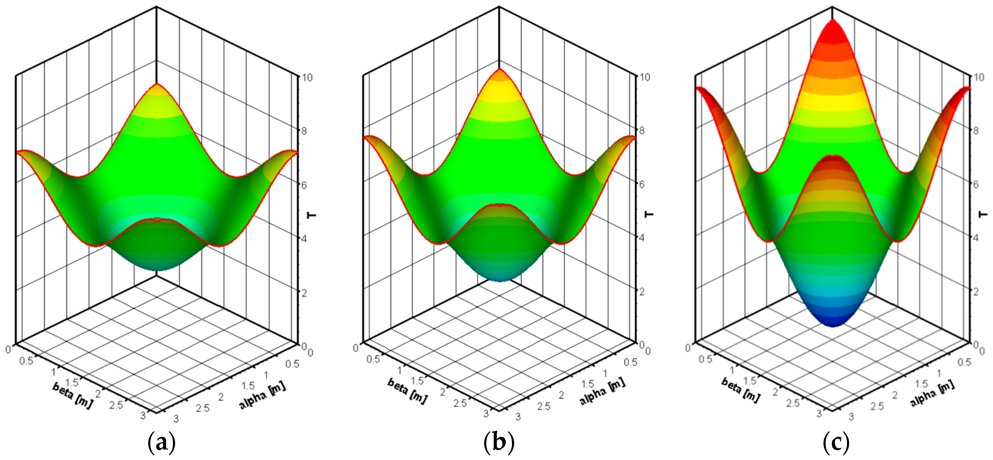
Figure 10.
Distribution of temperature over a time range from 0 s to 0.5 s.
Disclaimer/Publisher’s Note: The statements, opinions and data contained in all publications are solely those of the individual author(s) and contributor(s) and not of MDPI and/or the editor(s). MDPI and/or the editor(s) disclaim responsibility for any injury to people or property resulting from any ideas, methods, instructions or products referred to in the content. |
© 2024 by the authors. Licensee MDPI, Basel, Switzerland. This article is an open access article distributed under the terms and conditions of the Creative Commons Attribution (CC BY) license (https://creativecommons.org/licenses/by/4.0/).
Share and Cite
MDPI and ACS Style
Bağlan, İ.; Aslan, E. Analytical and Numerical Investigation of Two-Dimensional Heat Transfer with Periodic Boundary Conditions. Computation 2024, 12, 11. https://doi.org/10.3390/computation12010011
AMA Style
Bağlan İ, Aslan E. Analytical and Numerical Investigation of Two-Dimensional Heat Transfer with Periodic Boundary Conditions. Computation. 2024; 12(1):11. https://doi.org/10.3390/computation12010011
Chicago/Turabian StyleBağlan, İrem, and Erman Aslan. 2024. "Analytical and Numerical Investigation of Two-Dimensional Heat Transfer with Periodic Boundary Conditions" Computation 12, no. 1: 11. https://doi.org/10.3390/computation12010011
Note that from the first issue of 2016, this journal uses article numbers instead of page numbers. See further details here.