Article

Creation of a Simulated Sequence of Dynamic Susceptibility Contrast—Magnetic Resonance Imaging Brain Scans as a Tool to Verify the Quality of Methods for Diagnosing Diseases Affecting Brain Tissue Perfusion

by
Seweryn Lipiński
Department of Electrical Engineering, Power Engineering, Electronics and Automation, Faculty of Technical Sciences, University of Warmia and Mazury in Olsztyn, 10-036 Olsztyn, Poland
Computation 2024, 12(3), 54; https://doi.org/10.3390/computation12030054
Submission received: 25 January 2024 / Revised: 5 March 2024 / Accepted: 6 March 2024 / Published: 8 March 2024
(This article belongs to the Special Issue Computational Medical Image Analysis)

Abstract

:
DSC-MRI examination is one of the best methods of diagnosis for brain diseases. For this purpose, the so-called perfusion parameters are defined, of which the most used are CBF, CBV, and MTT. There are many approaches to determining these parameters, but regardless of the approach, there is a problem with the quality assessment of methods. To solve this problem, this article proposes virtual DSC-MRI brain examination, which consists of two steps. The first step is to create curves that are typical for DSC-MRI studies and characteristic of different brain regions, i.e., the gray and white matter, and blood vessels. Using perfusion descriptors, the curves are classified into three sets, which give us the model curves for each of the three regions. The curves corresponding to the perfusion of different regions of the brain in a suitable arrangement (consistent with human anatomy) form a model of the DSC-MRI examination. In the created model, one knows in advance the values of the complex perfusion parameters, as well as basic perfusion descriptors. The shown model study can be disturbed in a controlled manner—not only by adding noise, but also by determining the location of disturbances that are characteristic of specific brain diseases.

1. Introduction

DSC-MRI (Dynamic Susceptibility Contrast—Magnetic Resonance Imaging) is one of the most modern brain diagnostic methods. It allows for imaging perfusion, i.e., assessing the degree of blood supply and blood flow through tissues. As the perfusion changes in pathological lesions, DSC-MRI brain imaging allows for early diagnosis and the indication of the location of brain tissues that put patients at risk of pathologies such as cancerous tumors, damage resulting from a stroke, epilepsy, migraine headaches, dementia, Moyamoya disease, and many more [1,2,3,4,5].
In a DSC-MRI study, the response of the examined brain area is observed over time in the form of a sequence of MRI scans [6,7,8,9], after prior injection of a paramagnetic tracer (e.g., gadolinium-based chelates) into the bloodstream [8,9]. A tracer passes successively from the injection site, through the circulatory system and cerebral artery, and to the examined area (Region of Interest—ROI). Tracer flow causes changes in the measured MRI signal [8,9,10]. From the temporal sequence of MRI scans obtained during the examination, a temporal course of changes in the MRI signal is created for each pixel of the examined brain cross-section [10]. Its shape corresponds to changes in tracer concentration in the ROI. On this basis, the so-called perfusion parameters, containing diagnostic information, are calculated [11,12].
The most frequently used perfusion parameters are Cerebral Blood Volume (CBV), Cerebral Blood Flow (CBF), and Mean Transit Time (MTT). CBV can be calculated by assessing the area under the concentration–time curve. The most used approach to obtaining CBF is to utilize singular value decomposition (SVD) to estimate CBF through deconvolution of the arterial input function (AIF, i.e., the function that is an excitation for the ROI), while MTT is calculated by dividing CBV by CBF [2,9,11,12]. The basis of the diagnosis are so-called parametric images, which are maps of the values of perfusion parameters in the examined brain cross-section [13,14].
There are many approaches to determining perfusion parameters [12,13,15,16,17]. The most frequently used is the non-parametric approach, in which no internal structure of the system under study is assumed, and a specific regression function is fitted to the measurement data [12,16]. In the case of the parametric approach, a hypothesis is put forward regarding the functioning of the system under study, in the form of its model, which allows the parameters of such a model to be given a physical interpretation [17,18]. However, regardless of the approach used, there is a problem with assessing its quality and its comparison with others. This problem results from the small number of available measurement samples and the low quality of DSC-MRI data [19,20]. For this reason, tracer concentration curves are often simulated using various regression functions (e.g., gamma variate). Tracer concentration patterns in blood are usually created by selecting the parameters of the regression curve so that the perfusion parameters calculated on its basis agree with the literature values [16,21]. Consequently, the choice of a specific regression function affects the subsequent simulation results, favoring those methods in which perfusion parameters are estimated based on the same regression function.
Generally, in simulation-based DSC-MRI studies, a statistically significant set of curves is created, and then, affected in a specific way [19,21]. In most studies, complex perfusion parameters are determined, i.e., the above-mentioned CBF, CBV, and MTT. Meanwhile, in many cases, also related to the fact that DSC-MRI is used in an increasing range of brain diseases [1,2,3,4,5,6,7], it turns out that the basic perfusion descriptors may become more diagnostically useful [22,23]. The basic perfusion descriptors are those that can be determined directly from the tracer concentration curve, i.e., BAT (Bolus Arrival Time—the time of appearance of the tracer in the ROI), MPC (Maximum Peak Concentration—the maximum amplitude of the tracer concentration in the ROI), TTP (Time to Peak—the time taken to reach the maximum amplitude), and FWHM (Full Width at Half Maximum—the width of the tracer concentration curve at the height of half the maximum of the curve) [16,22]. This is significant because, especially in relation to time descriptors (BAT and TTP), the diagnosis depends not only on the descriptor value itself, but also on the connection of the measurement value with the location in the brain cross-section [24].
For brain tissue, there are two basic shapes of tracer concentration curves, i.e., for white and gray brain matter. In addition to signals from both tissues, signals from blood vessels are measured [11,13,14]. So, the aim of the first part of the article is to obtain three DSC-MRI curves characteristic of different brain regions, created not using the standard approach of simulating characteristic curves in the form of arbitrarily chosen regression functions, but from a set of measurement data from a clinical DSC-MRI study. The obtained characteristic curves will be then used to create a virtual DSC-MRI brain examination.
It will be possible to introduce known disturbances into the obtained model brain study (e.g., in the form of signals typical for pathologies such as tumor, stroke, etc.), and then, examine the effectiveness of their identification for various methods and computational algorithms. This will enable research to be conducted for various dimensions and shapes of pathological disorders and for various amounts of measurement disturbances.
To create such a virtual sequence of DSC-MRI scans covering the entire cross-section of the brain, model tracer concentration curves with a shape corresponding to perfusion in various brain regions, after conversion into a DSC-MRI measurement signal, must be appropriately arranged (corresponding to the anatomy of a specific brain cross-section).
The key motivation for creating a virtual DSC-MRI study in this form is the fact that, unlike the above-mentioned approach, in which we only simulate curves and not the entire sequence of images, in the proposed approach, we will know in advance the values of both complex perfusion parameters, as well as simple perfusion descriptors. Thanks to the possibility of introducing curves with a shape characteristic for various types of pathological lesions in a known place, their detectability can be evaluated. The model examination can be disturbed in a controlled way—noise with assumed characteristics can be introduced into the MRI signals [14,16,21]. The advantage of creating a sequence covering the entire cross-section of the brain is that we can also influence the entire sequence by disrupting the images created, not just the signals that form them. It is also possible to test the reliability of the methods when introducing pathologies of different diameters and profiles into the examination, which is impossible in the case of the classical approach, while the size of the detected pathology often implies the method of treatment (including the decision on surgical intervention), e.g., allows for the distinction between reversible and irreversible ischemia [23,25].

2. Materials

To maintain the uniformity of the input data, all clinical DSC-MRI measurements used for the creation of the virtual brain DSC-MRI examination were performed on a GE scanner with the following parameters of the sequence of scans: B = 1.5T, SE-EPI, 12 layers of size (slice thickness) 5–10 mm, 60 measurement points, TR (Repetition Time) = 1250–1610 ms, TE (Time Echo Delay) = 32–53 ms, Ts (sampling interval) = 1.43 s.
Gadopentetic acid (Gd-DTPA) was used as a paramagnetic contrast agent.
To maintain the anonymity of the subjects, 24 DSC-MRI sequences from adults assumed to be healthy (age 23–68) of both sexes were randomly selected from the available ones, which gave 1200 MRI images for analysis.
It should be noted that TR values, although varying, were considered appropriate for the model study, which results from the fact that since a short TR was below 700 ms, while a long TR was above 2000 ms [26], the range of 1250–1610 ms could be considered without deviations on either side.

3. Basic Perfusion Descriptors

Figure 1 shows the typical shape of the tracer concentration curve in the ROI [16,18].
Figure 1 also shows the basic perfusion descriptors that can be determined directly from this curve [14,16,18]:
  • The time of appearance of the tracer in the ROI—BAT (Bolus Arrival Time);
  • The maximum amplitude of the tracer concentration in the ROI—MPC (Maximum Peak Concentration);
  • The time taken to reach the maximum amplitude by the curve—TTP (Time to Peak);
  • The width of the tracer concentration curve at the height of half the maximum of the curve—FWHM (Full Width at Half Maximum).
The values of the descriptors characterizing the tracer concentration curve are different in different areas of the brain. Based on the literature study, the following were selected for further consideration: TTP, MPC, and FWHM [18,27]. The analysis of the values of these descriptors for the entire cross-section of the brain allows us to distinguish three subsets corresponding to three distinguished brain areas.
The following relationships exist between individual perfusion descriptors [16,28,29,30]:
  • M P C A > M P C G M > M P C W M ;
  • T T P W M > T T P G M > T T P A ;
  • F W H M W M > F W H M G M > F W H M A .
In the above relationships, WM represents white matter, GM gray matter, and A arteries.
The literature [29,30,31] presents classification methods using, among others, the above relationships to also assign each pixel of the brain slice to one of the three sets (WM, GM, or A). The research presented in this paper has a different goal, which is to obtain characteristic tracer concentration curves for three distinguished areas. Curves with a shape deviating from the characteristic shape (as shown in Figure 1) were identified as anomalous due to inappropriate perfusion parameters or due to excessive noise and were not included as components of the characteristic curves.

4. Method of Calculating Selected Perfusion Descriptors

In the three-compartment model of the process of the tracer passing through the circulatory system to the examined area in the brain, presented, e.g., in [17,18], AIF measurements, as well as measurements made in the ROI, basic regression functions were fitted, two- and three-exponential, respectively:
f r e g r A I F t = p 1 e p 2 t + p 3 e p 4 t ,
f r e g r R O I t = p 5 e p 6 t + p 7 e p 8 t + p 9 e p 10 t ,
where p 1 ÷ p 10 are simply the parameters of the above regression functions. These regression function parameters were estimated based on DSC-MRI measurements. The AIF parameters, i.e., p 1 ÷ p 4 , were the same for the whole sequence, while the parameters p 5 ÷ p 10 were calculated for each ROI separately, i.e., in accordance with the contrast agent concentration in a particular ROI.
The basic features of the parametric approach to calculating the most diagnostically important perfusion parameters (i.e., CBF, CBV, and MTT) are the avoidance of numerical deconvolution and the possibility of using stochastic filtering to improve the noise properties of the analyzed data. Both features are unique to the parametric approach [17,18,32]. Moreover, in the case of calculating the perfusion descriptors from Figure 1 using regression functions (1) and (2), these descriptors can be calculated directly using estimates of the parameters of the regression function.
The subject of interest in this work are the signals in the ROI (i.e., not the arterial input function). Therefore, a regression function in the form of Equation (2) was used, and the parameters were estimated. The regression function was fitted to first-pass samples, i.e., those corresponding to the first passage of the marker through the ROI [17,32]. For this purpose, the LS method and the Marquardt–Levenberg (M-L) algorithm were used.
After determining the estimates of the parameters of the regression function (3) for each considered curve, the perfusion descriptors were calculated as follows:
TTP and MPC
TTP, as the time in which the concentration curve reaches its maximum, is calculated by solving the following equation:
d f r e g R O I t d t = 0 ,
so, using Equation (2) as f r e g r R O I t , we obtain
( p 5 e p 6 t + p 7 e p 8 t + p 9 e p 10 t ) = 0 ,
p 5 p 6 e p 6 t p 7 p 8 e p 8 t p 9 p 10 e p 10 t = 0 .
The solution to Equation (5) is tMPC = TTP. According to Figure 1, the TTP descriptor clearly indicates the maximum MPC, and therefore,
M P C = f r e g r R O I t M P C .
FWHM
The FWHM descriptor value is calculated using the previously obtained MPC and TTP values. The value of the FWHM descriptor is defined as
F W H M = t 2 t 1 ,
where t1 and t2 are determined from the two following relationships:
f r e g r R O I t 1 = f r e g r R O I t M P C 2 ,   t < t M P C ,
f r e g r R O I t 2 = f r e g r R O I t M P C 2 ,   t > t M P C .
In other words, we calculate the time taken for the regression function to reach half of its maximum before reaching it (t1), as well as the time taken for the value of this function to fall back to half of its maximum after reaching it (t2). According to the definition of FWHM, the difference in these times gives us the exact value of this descriptor.

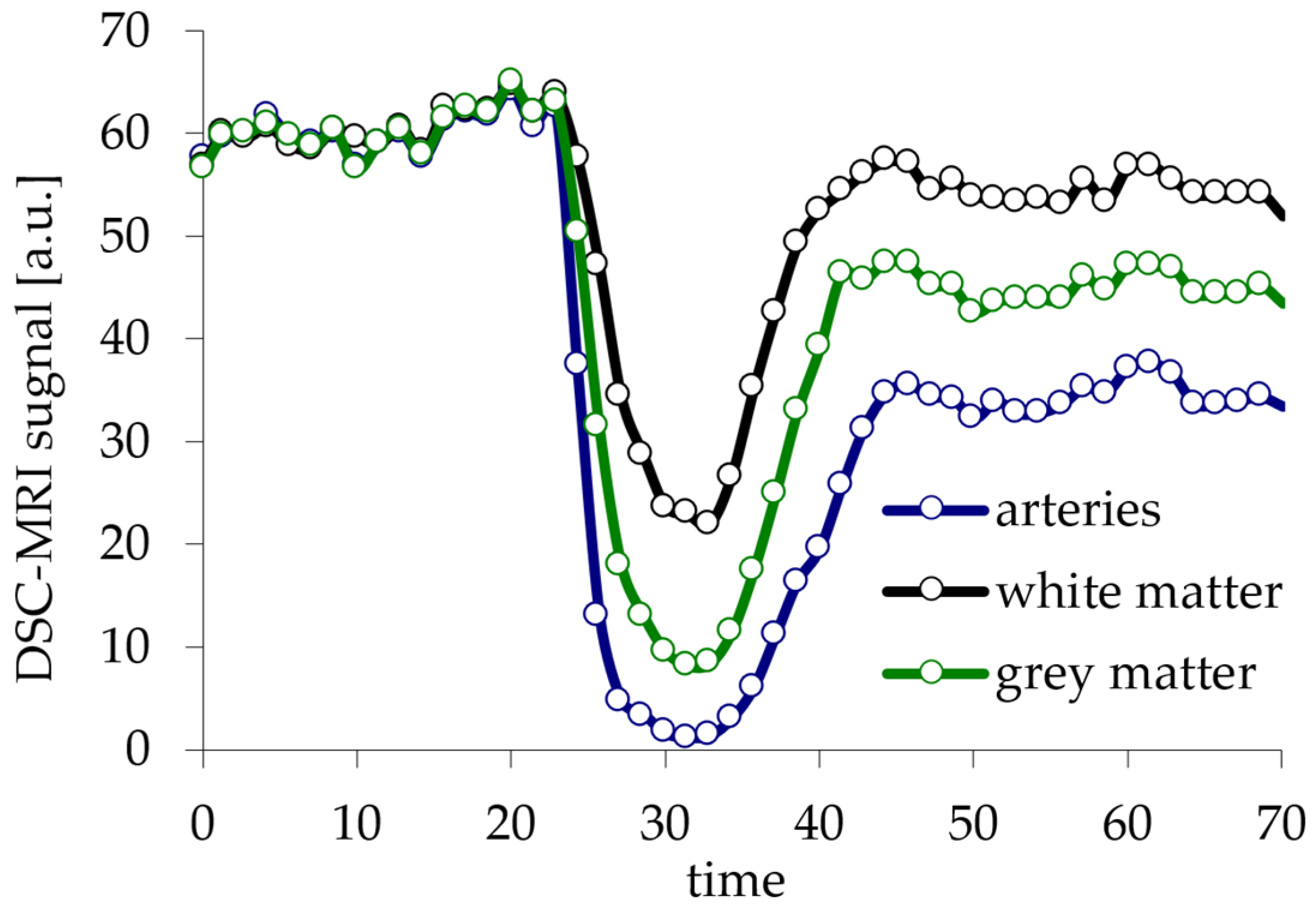
5. Creation and Verification of Model Curves

In the next step, each measurement curve was assigned a vector of previously selected descriptors characterizing it, related to the brain area based on previously shown relationships existing between individual perfusion descriptors, as given in [16,28,29,30]: D n = M P C n , T T P n , F W H M n , n = 1,2 , , N , where N is the number of all curves.
These vectors were assigned to appropriate sets, in this case, four. Three of them correspond to three brain areas, while the fourth is intended for non-standard curves that do not correspond to any of the three brain sets. The curves in the fourth set were too noisy, or they came from areas affected by the disease. Curves from this set were not components of characteristic signals—they were rejected, as they could influence the quality of the resulting model DSC-MRI study.
The unsupervised clustering method was used to divide the set of all curves. Generally, clustering is the task of dividing a multidimensional set of data (in this case, N vectors) characterized by a feature vector (in this case, a Dn vector of descriptors) into subsets in such a way that the elements of each subset are similar to each other while being as different as possible from elements belonging to other groups. For this purpose, this work uses the k-means algorithm, in which the data set is initially divided into a predetermined number of classes (in this case, equal to 4). Then, the obtained division is iteratively improved in such a way that some elements are transferred to other classes until the minimum variance within the obtained classes is obtained [33,34].
An unsupervised clustering algorithm was chosen so that the resulting sets of curves would not be subject to any arbitrarily selected thresholds or other factors that could influence the selection and, consequently, mismatch of the model curves to the brain region they are supposed to represent.
After clustering, characteristic curves were created by averaging each of the three obtained sets. Figure 2 shows the average curves from the first three sets, i.e., those containing measurements from the white and gray matter of the brain, and from blood vessels (arteries). These are the tracer concentration curves characteristic of particular brain regions.
Visual assessment of the averaged curves from Figure 2 allows us to initially conclude that the selected classification method works properly. The differences between them correspond to those known from the literature [11,13,14,28,29].
Better verification of the quality of the obtained curves can be achieved by comparing the CBV parameter values calculated for each of the obtained characteristic curves with the values known from the literature. The choice of the CBV for this purpose was dictated by the fact that of the three complex perfusion parameters (i.e., CBF, CBV, and MTT), this one is the most computationally explicit and, in some cases, it is possible to use a regional relative description of CBV without knowing the arterial input function [35]. CBV is, by definition, given as [11,13,14,36]
C B V = 0 C R O I t d t 0 C A I F t d t ,
where C R O I t d t and C A I F t d t are the tracer concentration curves for the ROI and for the AIF, respectively.
As follows from Equation (10), the absolute value of CBV depends on the arterial input function. The value of the denominator (i.e., integral of the arterial input function) is the same for each pixel of the brain cross-section, so to verify the quality of the obtained characteristic curves, the CBV ratios for the three individual brain regions can be used. This will make the obtained results independent of the possible impact of the arterial input function on their quality.
So, CBVA/CBVGM and CBVGM/CBVWM were calculated, and the obtained results were compared with values obtained from six different clinical studies [29,31,36,37,38,39]. The results are shown in Table 1.
The results presented in Table 1 show that the proposed approach enables very good compliance of the perfusion parameters with those published in the literature. This means that the curves shown in Figure 2 can be used as tracer concentration curves specific to the white and gray matter of the brain and to blood vessels. It is worth noting that only the authors of [29] present the CBVA/CBVGM ratio. In the same paper, Artzi et al. [29] point out that it is impossible to compare the result obtained by them with the literature values, as such values are not published; however, a comparison of the highest curve in Figure 2 with the curves obtained in arteries and presented, for example, in the works [11,13,14,28,29] shows very good compliance between the shapes of these curves. The lack of other CBVA values in the literature can probably be explained by the fact that, in general, determining the position of arteries in a cross-section of the brain is a difficult task, and in fact, it is most often only used to determine curves that can be candidates for AIF [18,27].
However, the obtained value of the CBVGM/CBVWM ratio is consistent with five of the six clinical trial results shown. The result from [31] differs from others, which may be due to the use of a different calculation method or the fact that in many studies, the ROI selection is performed manually. This may lead to the over- or under-estimation of values due to the inaccurate marking of gray- and white-matter regions, or by incorrectly including measurements from vessels in these regions.
The tracer concentration curves shown in Figure 2 can be used to evaluate and compare methods for calculating complex perfusion parameters. Their main advantage is the fact that they were obtained based on an actual DSC-MRI examination of the brain, and not using the standard approach of simulating regression curves. However, this is not their only possible application. The next part of this article will show other possibilities of using the obtained characteristic curves, i.e., creating a simulated DSC-MRI brain examination.

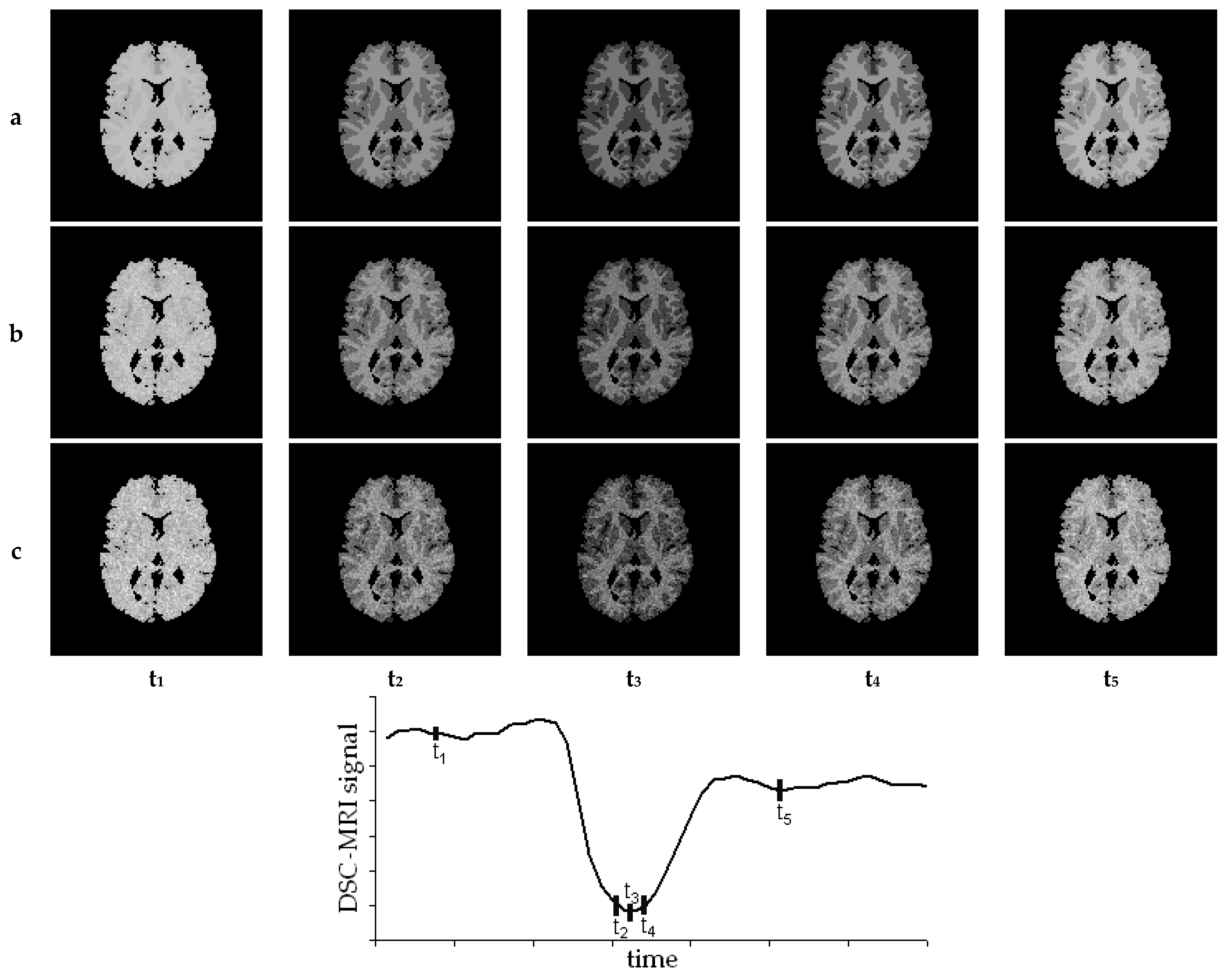
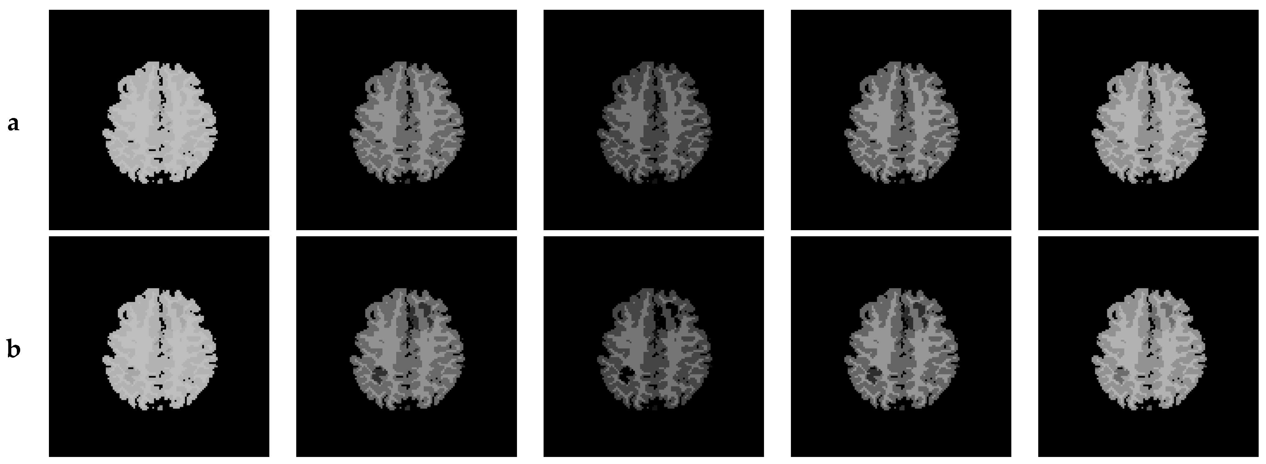
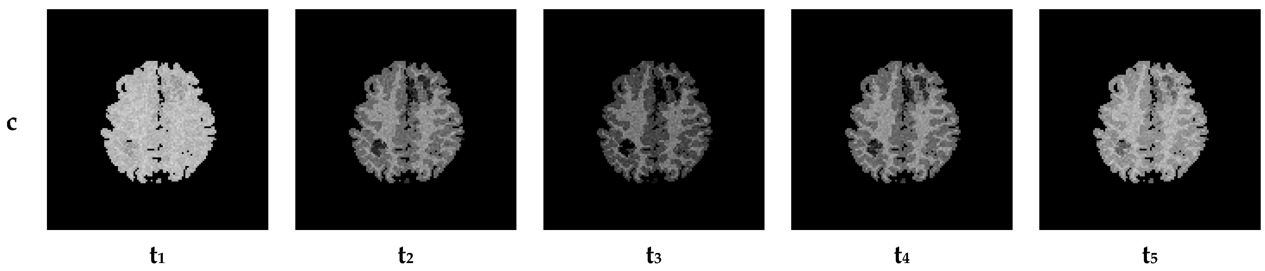
6. Creation of DSC-MRI Measurement Curves and a Brain Anatomy Model

From the c(t) tracer concentration curve in the blood, the DSC-MRI measurement signal S(t) is obtained from the following relationship [40]:
S t = S 0 e κ c ( t ) T E
where S0 is the amplitude of the measurement signal before contrast administration, and κ is the proportionality coefficient (depending on the properties of the tissue and measurement conditions resulting from the device used).
Figure 3 shows model DSC-MRI signals calculated using Equation (11) and based on the previously obtained model tracer concentration curves for individual brain regions. The DSC-MRI measurements used to create the model curves consisted of 50 scans, so this was the resolution of the model study.
To create the model study, a physiological base was needed, i.e., the arrangement of individual tissues in a cross-section of the brain. The BrainWeb database was used for this purpose [41,42,43,44]. This database provides, among others, 20 virtual static brain MRI images [43]. The MRI simulator described in [44] includes blood vessels, which, combined with the model DSC-MRI measurement signals from Figure 3, makes it possible to use it to create a model series of dynamic brain images including blood vessels, without the need to obtain an anatomical base from the segmentation of brain areas from other imaging studies.
It should be noted that at this stage, changes in the brain resulting from aging (like the WM/GM ratio) or sex differences should be considered if necessary [45,46,47].
Figure 4 shows where the gray (b) and white (c) matter of the brain and blood vessels (d) are located in two selected brain cross-sections (a). The maps shown in Figure 4b–d allow for the appropriate location of the model DSC-MRI signals, and thus, the creation of a simulation of a DSC-MRI study, consisting of a sequence of scans with the same parameters as the actual studies constituting the basis for obtaining the model DSC-MRI signals.

7. Results—Exemplary DSC-MRI Study Models

Figure 5 shows five selected exemplary scans from a model DSC-MRI study created based on cross-section P of Figure 4: one scan from before the tracer appeared (t1), one when the tracer reached its maximum value (t3), two adjacent to it (t2 and t4), and one after tracer passing, i.e., during the recirculation (t5). One study (row a) contains no noise, and two others (rows b and c) are artificially noised. The DSC-MRI signals were distorted using Gaussian white noise at levels of SNR of 25 dB (b) and 20 dB (c).
DSC-MRI examination is used for the diagnosis of an increasing range of brain diseases. Each disease (as well as its stage) has more or less specific characteristics and, in a peculiar way, affects simple and complex perfusion parameters [1,14,15,22,48]. Therefore, the introduction of a pathology with a specific diameter and profile into a model sequence can show how effective each approach to calculating perfusion parameters is in terms of detecting a specific pathology. Figure 6 shows the location of two pathologies with different dimensions introduced into the model DSC-MRI examination.
A pathology with the shape shown in Figure 6 was introduced into a model study based on the brain cross-section from row L of Figure 4. The model DSC-MRI signals were modified based on the thresholds imposed on the perfusion descriptors proposed by Grandin et al. [23] to detect ischemic cerebral infarction. The DSC-MRI examination created in this way is shown in Figure 7. The scans were selected analogously to those from Figure 5. The first sequence (a) does not contain noise or a pathology, the second one (b) has a pathology introduced as described above, and the third one (c) contains a pathology and is also disturbed by noise at an SNR level of 25 dB.
Figure 8 shows maps of the three most important perfusion parameters, i.e., CBV, CBF, and MTT, calculated based on the sequence shown in Figure 7c.
As can be seen in Figure 8, the introduced pathologies in the parametric images are clearly observable and consistent with the shape of the pathologies shown in Figure 6. In the case shown, both pathologies are relatively obvious, and they also have a large diameter; therefore, for a diagnostician, it would be hard not to notice the impact of the disease on the parameter map. However, the pathological changes appearing in the brain cross-section may have a completely different shape (irregular) and a much smaller diameter, and their impact on the tracer concentration curve may also be much more subtle. In such cases, it is extremely desirable that the perfusion parameter map assessed by the doctor is as reliable as possible. The proposed virtual study can be used as a tool for this purpose. With its help, it is possible to objectively compare different approaches to calculating perfusion parameters by checking how the obtained parametric maps correlate with a known pathological change introduced in a specific location.

8. Discussion and Conclusions

This article proposes the creation of a simulated DSC-MRI examination. Curves corresponding to the perfusion of various brain regions in an appropriate arrangement (corresponding to the anatomy of a specific brain cross-section) create model DSC-MRI studies. Using sequences created in this way, we know in advance the values of both complex perfusion parameters and their simple descriptors. We can disrupt the model study in a controlled way—not only by introducing disturbances of the assumed size and characteristics to the DSC-MRI signals, but also by influencing their location (and distribution) in the brain cross-section(s). Other types of interference that can be introduced into such sequences, typical for image data, are blurring, geometric shifts between subsequent images in the sequence, etc. Assessment of the resistance of the methods for determining perfusion parameters to this type of interference is impossible when the interference is introduced only to DSC-MRI signals, i.e., as in the approach classically proposed in the literature. The described research model will allow us to reliably and objectively, while considering the type of brain tissue (white and gray matter), assess the quality of various approaches to calculating perfusion parameters.
Additionally, disturbed signals characteristic of specific pathologies can be introduced into such a sequence. Then, an additional criterion for assessing the approach to determining perfusion parameters is to check the threshold (this threshold may be, for example, the diameter of the introduced disorder) for detecting perfusion disorders in the presence of various types of disturbances, either automatically or indirectly, through the assessment of the diagnosing doctor based on a map of specific parameters.
The one limitation of the proposed approach is the fact that reliable data are needed on the impact of each specific disease on the flow of the tracer through the brain tissue, so that the disorders introduced into the virtual study reflect reality.
Another limitation of the proposed approach is the fact that if an analogous model study for long or short TR was to be created, a different set of DSC-MRI studies must be used for the creation of model curves.
It is also worth emphasizing that this study focuses on a method that can be considered invasive, as it involves tracer injection, while in recent years, non-invasive methods of brain perfusion imaging have been gaining popularity, with particular emphasis on Arterial Spin Labeling (ASL) perfusion MRI [49,50,51]. Since the use of this method is based on a different principle, the described approach cannot be used to create an analogous research model.

Funding

This research received no external funding.

Data Availability Statement

The dataset is available on request from the author.

Conflicts of Interest

The author declares no conflicts of interest.

References

  1. Forsting, M.; Weber, J. MR perfusion imaging: A tool for more than a stroke. Eur. Radiol. Suppl. 2004, 14 (Suppl. 5), M2–M7. [Google Scholar]
  2. Lanzman, B.; Heit, J. Advanced MRI measures of cerebral perfusion and their clinical applications. Top. Magn. Reson. Imaging 2017, 26, 83–90. [Google Scholar] [CrossRef] [PubMed]
  3. Lee, H.; Fu, J.F.; Gaudet, K.; Bryant, A.G.; Price, J.C.; Bennett, R.E.; Johnson, K.A.; Hyman, B.T.; Hedden, T.; Salat, D.H.; et al. Aberrant vascular architecture in the hippocampus correlates with tau burden in mild cognitive impairment and Alzheimer’s disease. J. Cereb. Blood Flow Metab. 2023, 0271678X231216144. [Google Scholar] [CrossRef]
  4. Petrella, J.R.; Provenzale, J.M. MR Perfusion Imaging of the Brain: Techniques and Applications. Am. J. Roentgenol. 2000, 175, 207–219. [Google Scholar] [CrossRef] [PubMed]
  5. Zuloaga, K.L.; Zhang, W.; Yeiser, L.A.; Stewart, B.; Kukino, A.; Nie, X.; Roese, N.E.; Grafe, M.R.; Pike, M.M.; Raber, J.; et al. Neurobehavioral and imaging correlates of hippocampal atrophy in a mouse model of vascular cognitive impairment. Transl. Stroke Res. 2015, 6, 390–398. [Google Scholar] [CrossRef] [PubMed]
  6. Bakhtiari, A.; Vestergaard, M.B.; Benedek, K.; Fagerlund, B.; Mortensen, E.L.; Osler, M.; Lauritzen, M.; Larsson, H.B.W.; Lindberg, U. Changes in hippocampal volume during a preceding 10-year period do not correlate with cognitive performance and hippocampal blood–brain barrier permeability in cognitively normal late-middle-aged men. GeroScience 2023, 45, 1161–1175. [Google Scholar] [CrossRef]
  7. Choi, J.D.; Moon, Y.; Kim, H.J.; Yim, Y.; Lee, S.; Moon, W.J. Choroid plexus volume and permeability at brain MRI within the Alzheimer disease clinical spectrum. Radiology 2022, 304, 635–645. [Google Scholar] [CrossRef]
  8. Gordon, Y.; Partovi, S.; Müller-Eschner, M.; Amarteifio, E.; Bäuerle, T.; Weber, M.A.; Kauczor, H.-U.; Rengier, F. Dynamic contrast-enhanced magnetic resonance imaging: Fundamentals and application to the evaluation of the peripheral perfusion. Cardiovasc. Diagn. Ther. 2014, 4, 147. [Google Scholar]
  9. Koh, T.S.; Bisdas, S.; Koh, D.M.; Thng, C.H. Fundamentals of tracer kinetics for dynamic contrast-enhanced MRI. J. Magn. Reson. Imaging 2011, 34, 1262–1276. [Google Scholar] [CrossRef]
  10. Kalicka, R.; Lipiński, S. A fast method of separation of the noisy background from the head-cross section in the sequence of MRI scans. Biocybern. Biomed. Eng. 2010, 30, 15–27. [Google Scholar]
  11. Calamante, F.; Thomas, D.L.; Pell, G.S.; Wiersma, J.; Turner, R. Measuring Cerebral Blood Flow Using Magnetic Resonance Imaging Techniques. J. Cereb. Blood Flow. Metab. 1999, 19, 701–735. [Google Scholar] [CrossRef] [PubMed]
  12. Jackson, D. Analysis of dynamic contrast enhanced MRI. Br. J. Radiol. 2004, 77, S154–S166. [Google Scholar] [CrossRef] [PubMed]
  13. van Osch, T. Evaluation of Cerebral Hemodynamics by Quantitative Perfusion MRI; PrintPartners Ipskamp: Enschede, The Netherlands, 2002. [Google Scholar]
  14. Sorensen, A.G.; Reimer, P. Cerebral MR Perfusion Imaging. Principles and Current Applications; Georg Thieme Verlag: Stuttgart, Germany, 2000. [Google Scholar]
  15. Kane, I.; Carpenter, T.; Chappell, F.; Rivers, C.; Armitage, P.; Sandercock, P.; Wardlaw, J. Comparison of 10 Different Magnetic Resonance Perfusion Imaging Processing Methods in Acute Ischemic Stroke. Stroke 2007, 38, 3158–3164. [Google Scholar] [CrossRef]
  16. Perthen, J.E.; Calamante, F.; Gadian, D.G.; Connelly, A. Is Quantification of Bolus Tracking MRI Reliable Without Deconvolution? Magn. Reson. Med. 2002, 47, 61–67. [Google Scholar] [CrossRef] [PubMed]
  17. Kalicka, R.; Pietrenko-Dąbrowska, A. Parametric Modeling of DSC-MRI Data with Stochastic Filtration and Optimal Input Design Versus Non-Parametric Modeling. Ann. Biomed. Eng. 2007, 35, 453–464. [Google Scholar] [CrossRef] [PubMed]
  18. Lipiński, S.; Kalicka, R. Automatic selection of arterial input function in DSC-MRI measurements for calculation of brain perfusion parameters using parametric modelling. Math. Model. Nat. Phenom. 2018, 13, 58. [Google Scholar] [CrossRef]
  19. Salluzzi, M.; Frayne, R.; Smith, M.R. Is correction necessary when clinically determining quantitative cerebral perfusion parameters from multi-slice dynamic susceptibility contrast MR studies? Phys. Med. Biol. 2006, 51, 407–424. [Google Scholar] [CrossRef]
  20. Smith, M.R.; Lu, H.; Frayne, R. Signal-to-Noise Ratio Effects in Quantitative Cerebral perfusion Using Dynamic Susceptibility Contrast Agents. Magn. Reson. Med. 2003, 49, 122–128. [Google Scholar] [CrossRef]
  21. Knutsson, L.; Stahlberg, F.; Wirestam, R. Aspects on the accuracy of cerebral perfusion parameters obtained by dynamic susceptibility contrast MRI: A simulation study. Magn. Reson. Imaging 2004, 22, 789–798. [Google Scholar] [CrossRef]
  22. Calamante, F.; Ganesan, V.; Kirkham, F.J.; Chir, B.; Jan, W.; Chong, W.K.; Gadian, D.G.; Connelly, A. MR Perfusion Imaging in Moyamoya Syndrome. Stroke 2001, 32, 2810–2816. [Google Scholar] [CrossRef]
  23. Grandin, C.B.; Duprez, T.P.; Smith, A.M.; Oppenheim, C.; Peeters, A.; Robert, A.R.; Cosnard, G. Which MR-derived perfusion parameters are the best predictors of infarct growth in hyperacute stroke? Comparative study between relative and quantitative measurements. Radiology 2002, 223, 361–370. [Google Scholar] [CrossRef] [PubMed]
  24. Akella, N.S.; Twieg, D.B.; Mikkelsen, T.; Hochberg, F.H.; Grossman, S.; Cloud, G.A.; Nabors, L.B. Assessment of Brain Tumor Angiogenesis Inhibitors Using Perfusion Magnetic Resonance Imaging: Quality and Analysis Results of a Phase I Trial. J. Magn. Reson. Imaging 2004, 20, 913–922. [Google Scholar] [CrossRef]
  25. Wintermark, M.; Sesay, M.; Barbier, E.; Borbély, K.; Dillon, W.P.; Eastwood, J.D.; Glenn, T.C.; Grandin, C.B.; Pedraza, S.; Soustiel, J.-F.; et al. Comparative Overview of Brain Perfusion Imaging Techniques. Stroke 2005, 36, e83–e99. [Google Scholar] [CrossRef]
  26. Bitar, R.; Leung, G.; Perng, R.; Tadros, S.; Moody, A.R.; Sarrazin, J.; McGregor, C.; Christakis, M.; Symons, S.; Nelson, A.; et al. MR pulse sequences: What every radiologist wants to know but is afraid to ask. Radiographics 2006, 26, 513–537. [Google Scholar] [CrossRef]
  27. Mouridsen, K.; Christensen, S.; Gyldensted, L.; Ostergaard, L. Automatic Selection of Arterial Input Function Using Cluster Analysis. Magn. Reson. Med. 2006, 55, 524–531. [Google Scholar] [CrossRef] [PubMed]
  28. Koshimoto, Y.; Yamada, H.; Kimura, H.; Maeda, M.; Tsuchida, C.; Kawamura, Y.; Ishii, Y. Quantitative Analysis of Cerebral Microvascular Hemodynamics with T2-Weighted Dynamic MR Imaging. J. Magn. Reson. Imaging 1999, 9, 462–467. [Google Scholar] [CrossRef]
  29. Artzi, M.; Aizenstein, O.; Hendler, T.; Bashat, D.B. Unsupervised multiparametric classification of dynamic susceptibility contrast imaging: Study of a healthy brain. Neuroimage 2011, 56, 858–864. [Google Scholar] [CrossRef] [PubMed]
  30. Kao, Y.-H.; Guo, W.-Y.; Wu, Y.-T.; Liu, K.-C.; Chai, W.-Y.; Lin, C.-Y.; Hwang, Y.-S.; Liou, A.J.-K.; Wu, H.-M.; Cheng, H.-C.; et al. Hemodynamic Segmentation of MR Brain Perfusion Images Using Independent Component Analysis, Thresholding, and Bayesian Estimation. Magn. Reson. Med. 2003, 49, 885–894. [Google Scholar] [CrossRef]
  31. Bjornerud, A.; Emblem, K.E. A fully automated method for quantitative cerebral hemodynamic analysis using DSC-MRI. J. Cereb. Blood Flow. Metab. 2010, 30, 1066–1078. [Google Scholar] [CrossRef]
  32. Kalicka, R.; Lipiński, S. Valuation of usefulness of Kalman filtration to improve noise properties of DSC-MRI brain research data. Meas. Automat. Monit. 2008, 54, 118–121. [Google Scholar]
  33. Theodoridis, S.; Pikrakis, A.; Kotroumbas, K.; Cavouras, D. An Introduction to Pattern Recognition: A MATLAB Approach; Elsevier Academic Press: Cambridge, MA, USA, 2010. [Google Scholar]
  34. Jain, A.K.; Duin, R.P.W.; Mao, J. Statistical Pattern Recognition: A review. IEEE Trans. Pattern Anal. 2000, 22, 4–37. [Google Scholar] [CrossRef]
  35. Calamante, F.; Gadian, D.G.; Connelly, A. Quantification of Perfusion Using Bolus Tracking Magnetic Resonance Imaging in Stroke: Assumptions, Limitations, and Potential Implications for Clinical Use. Stroke 2002, 33, 1146–1151. [Google Scholar] [CrossRef]
  36. Ibaraki, M.; Ito, H.; Shimosegawa, E.; Toyoshima, H.; Ishigame, K.; Takahashi, K.; Kanno, I.; Miura, S. Cerebral vascular mean transit time in healthy humans: A comparative study with PET and dynamic susceptibility contrast-enhanced MRI. J. Cereb. Blood Flow. Metab. 2007, 27, 404–413. [Google Scholar] [CrossRef] [PubMed]
  37. Schreiber, W.G.; Guckel, F.; Stritzke, P.; Schmiedek, P.; Schwartz, A.; Brix, G. Cerebral Blood Flow and Cerebrovascular Reserve Capacity: Estimation by Dynamic Magnetic Resonance Imaging. J. Cereb. Blood Flow. Metab. 1998, 18, 1143–1156. [Google Scholar] [CrossRef]
  38. Wenz, F.; Rempp, K.; Brix, G.; Knopp, M.V.; Gückel, F.; Hess, T.; van Kaick, G. Age dependency of the regional cerebral blood volume (rCBV) measured with dynamic susceptibility contrast MR imaging (DSC). Magn. Reson. Imaging 1996, 14, 157–162. [Google Scholar] [CrossRef]
  39. Fuss, M.; Wenz, F.; Scholdei, R.; Essig, M.; Debus, J.; Knopp, M.V.; Wannenmacher, M. Radiation-induced regional cerebral blood volume (rCBV) changes in normal brain and low-grade astrocytomas: Quantification and time and dose-dependent occurrence. Int. J. Radiat. Oncol. Biol. Phys. 2000, 48, 53–58. [Google Scholar] [CrossRef]
  40. Ostergaard, L.; Weisskoff, R.M.; Chesler, D.A.; Gyldensted, C.; Rosen, B.R. High resolution Measurement of Cerebral Blood Flow using Intravascular Tracer Bolus Passages. Part I: Mathematical Approach and Statistical Analysis. Magn. Reson. Med. 1996, 36, 715–725. [Google Scholar] [CrossRef] [PubMed]
  41. Cocosco, C.A.; Kollokian, V.; Kwan, R.K.-S.; Evans, A.C. BrainWeb: Online Interface to a 3D MRI Simulated Brain Database. NeuroImage 1997, 5, 1996. [Google Scholar]
  42. Kwan, R.K.-S.; Evans, A.C.; Pike, G.B. An Extensible MRI Simulator for Post-Processing Evaluation. Lect. Notes Comput. Sci. 1996, 1131, 135–140. [Google Scholar]
  43. Aubert-Broche, B.; Griffin, M.; Pike, G.B.; Evans, A.C.; Collins, D.L. Twenty new digital brain phantoms for creation of validation image data bases. IEEE Trans. Med. Imaging 2006, 25, 1410–1416. [Google Scholar] [CrossRef]
  44. Aubert-Broche, B.; Evans, A.C.; Collins, D.L. A new improved version of the realistic digital brain phantom. NeuroImage 2006, 32, 138–145. [Google Scholar] [CrossRef]
  45. Fujita, S.; Mori, S.; Onda, K.; Hanaoka, S.; Nomura, Y.; Nakao, T.; Yoshikawa, T.; Takao, H.; Hayashi, N.; Abe, O. Characterization of brain volume changes in aging individuals with normal cognition using serial magnetic resonance imaging. JAMA Netw. Open 2023, 6, e2318153. [Google Scholar] [CrossRef] [PubMed]
  46. Gómez-Ramírez, J.; Fernández-Blázquez, M.A.; González-Rosa, J.J. A causal analysis of the effect of age and sex differences on brain atrophy in the elderly brain. Life 2022, 12, 1586. [Google Scholar] [CrossRef] [PubMed]
  47. Usui, K.; Yoshimura, T.; Tang, M.; Sugimori, H. Age Estimation from Brain Magnetic Resonance Images Using Deep Learning Techniques in Extensive Age Range. Appl. Sci. 2023, 13, 1753. [Google Scholar] [CrossRef]
  48. Tofts, P. (Ed.) Quantitative MRI of the Brain. Measuring Changes Caused by Disease; John Wiley and Sons: Hoboken, NJ, USA, 2004. [Google Scholar]
  49. Bambach, S.; Smith, M.; Morris, P.P.; Campeau, N.G.; Ho, M.L. Arterial spin labeling applications in pediatric and adult neurologic disorders. J. Magn. Reson. Imaging 2022, 55, 698–719. [Google Scholar] [CrossRef] [PubMed]
  50. Iutaka, T.; de Freitas, M.B.; Omar, S.S.; Scortegagna, F.A.; Nael, K.; Nunes, R.H.; Pacheco, F.T.; Maia Júnior, A.C.M.; do Amaral, L.L.F.; da Rocha, A.J. Arterial spin labeling: Techniques, clinical applications, and interpretation. Radiographics 2022, 43, e220088. [Google Scholar] [CrossRef] [PubMed]
  51. Qin, Q.; Alsop, D.C.; Bolar, D.S.; Hernandez-Garcia, L.; Meakin, J.; Liu, D.; Nayak, K.S.; Schmid, S.; van Osch, M.J.P.; Wong, E.C.; et al. Velocity-selective arterial spin labeling perfusion MRI: A review of the state of the art and recommendations for clinical implementation. Magn. Reson. Med. 2022, 88, 1528–1547. [Google Scholar] [CrossRef]
Figure 1. Tracer concentration curve with selected basic perfusion descriptors.
Computation 12 00054 g001
Figure 2. Contrast agent concentration curves characteristic of three brain regions. On these curves, we can identify baseline (0–24 s), first-pass of contrast agent (24–40 s), and contract agent recirculation (40–60 s).
Computation 12 00054 g002
Figure 3. DSC-MRI signals derived from model contrast agent concentration curves for each of three brain regions: gray matter, white matter, and arteries.
Computation 12 00054 g003
Figure 4. Brain cross-sections serving as bases of two models of DSC-MRI examinations, (a) and localization of gray matter (b), white matter (c), and arteries (d) on these cross-sections.
Computation 12 00054 g004
Figure 5. Representative scans from exemplary model DSC-MRI examination: sequence of scans for healthy brain (a) and the same sequence with low (b) and high (c) noise content.
Computation 12 00054 g005
Figure 6. Shapes (a) and localizations (b) of the pathologies introduced into the model research.
Computation 12 00054 g006
Figure 7. Representative scans from different exemplary model DSC-MRI examinations: healthy brain (a), brain with inserted pathologies (b), and brain with two pathologies and noise content (c).
Computation 12 00054 g007aComputation 12 00054 g007b
Figure 8. CBV, CBF, and MTT perfusion maps obtained based on the model sequence shown in Figure 7c.
Computation 12 00054 g008
Table 1. Comparison of results obtained based on curves characteristic of three brain regions obtained in this study with published parameter values obtained from clinical studies.
CBVA/CBVGMCBVGM/CBVWM
Based on the Model Curves
Presented in This Work
1.972.19
Artzi et al. [29]1.60–2.102–2.4
Bjornerud and Emblem [31](not investigated)1.60–1.98 or 1.74–2.18
(depending on the calculation method)
Ibaraki et al. [36](not investigated)1.60–2.40 or 2.30–2.50
(depending on the ROI)
Schreiber et al. [37](not investigated)1.90–2.30
Wenz et al. [38](not investigated)1.60–2.60
Fuss et al. [39](not investigated)1.50–2.80
Disclaimer/Publisher’s Note: The statements, opinions and data contained in all publications are solely those of the individual author(s) and contributor(s) and not of MDPI and/or the editor(s). MDPI and/or the editor(s) disclaim responsibility for any injury to people or property resulting from any ideas, methods, instructions or products referred to in the content.

