CFD and Experimental Study on the Effect of Progressive Heating on Fluid Flow inside a Thermal Wind Tunnel

Abstract

A detailed Computational Fluid Dynamics (CFD) and experimental investigation into characterizing the fluid flow and thermal profiles in a wind tunnel was carried out, highlighting the effect of progressive heating on the non-uniformity flow profile of air. Using controllable electrical heating elements, the operating temperatures in the test-section were gradually increased in order to determine its influence on the subsequent velocity and thermal profiles found inside the test-section. The numerical study was carried out using CFD FLUENT code, alongside validating the experimental results. Good correlation was observed as the comparison yielded a mean error of 6.4% for the air velocity parameter and 2.3% for the air temperature parameter between the two techniques. The good correlation established between the numerically predicted and experimentally tested results identified broad scope for using the advanced computational capabilities of CFD applicable to the thermal modeling of wind tunnels. For a constant temperature process, the non-uniformity and turbulence intensity in the test section was 0.9% and 0.5%, which is under the recommended guidelines for wind tunnels. The findings revealed that the increase in temperature from 20 °C to 50 °C reduced the velocity by 15.2% inside the test section.

1. Introduction

Wind tunnels are a significant research apparatus used in aerodynamic investigations to study the effects of air moving past solid objects. In order to avoid the high expenditure of design and adaptation, CFD is often used to precisely comprehend the flow profiles within the tunnel environment. The common objective for most wind tunnels is to obtain a flow in the test section that is a parallel steady flow with uniform speed throughout the test section [1,2,3] The fundamental principles used to model low-speed aerodynamic flows include mass conservation, force and motion relating to Newton’s Second Law and energy exchanges governed by the First Law of Thermodynamics. In considering low-speed flows, the assumption of incompressible flow is often adopted to determine the correlation with respect to full-scale structural dynamic characteristics [4,5,6,7]. To account for accurate simulation procedures, viable numerical codes have been developed and applied to establish mathematical models involving flow and turbulence [8].

Apart from the overall flow profile, a precise evaluation of turbulence in wind tunnels is of paramount importance, while designing and commissioning the test-section. Viscous and thermal boundary layers have been experimentally and theoretically investigated in-depth in the past. The source of turbulence in wind tunnels can be briefly divided in two parts; turbulence due to eddies (vortex shedding, boundary layer, shear stress, and secondary flows) and noise (mechanical, vibration and aerodynamic) [9,10,11].

In the past, wind tunnels have been designed to produce layers or continuous stratification by passing the air through an upstream heat exchanger, injection of heated air or a dense gas, or the use of a thermal boundary layer grown over long segments of heated or cooled surfaces [12]. In addition, the influence of operating temperature produced by friction of the fan blades and electrical heating on these parameters is of significant importance when working with stratified flows in order to determine the actual flow profiles inside the test section while conducting wind tunnel experimentation.

Previous Related Work

Studies on comprehending the behavior of fluid flows using experimental and numerical methods have resulted in continuous advancement of knowledge in characterizing wind tunnels for wind engineering and aerodynamics. Diana et al. [13] establishes the non-uniformity and turbulence behavior of mean velocity inside the test-section of a wind tunnel designed for civil and aeronautical applications. The findings have depicted that both non-uniformity and turbulence were recorded under 2% in the civil test-section, while the smaller test-section used in aeronautics recorded non-uniformity and turbulence values of under 0.2%.

A numerical methodology for modeling flow conditions in a closed-loop wind tunnel was developed by Moonen et al. [14]. A full-scale CFD model of the actual wind tunnel was considered. The study combined structured grid and unstructured grid in generating the computational domain, those sections of the wind tunnels that are of simple geometry are meshed with prismatic cells and complex geometries such as the guide vane and screens are meshed with tetrahedral cells. Steady-state and three-dimensional CFD simulations, using standard and realizable k-epsilon turbulence equations models, were carried out to determine the total pressure loss and flow rate in the test section. The numerical model was validated against experimentation on the wind tunnel. The findings revealed an error percentage of 10% between the measured and CFD predicted values for air velocities. The performance of the numerical model for predicting turbulence intensities produced satisfying results with a relative error of less than 20%.

Further work by Moonen et al. [15] included a detailed determination of the flow quality in the test section. The work developed six corresponding indices for the evaluation of the three-dimensional flow quality in the test section. The first index calculated uniformity of the velocity flow field, while the other indices are correlated to imperfections in the flow field such as the skewness and flow angularity. The three-dimensional Reynolds-averaged Navier–Stokes (RANS) equations and the continuity equation were solved using a commercial CFD code that employs the control-volume technique. The work depicted the effect of adding guide vanes and mesh screens in the contraction nozzle to improve the flow quality in the working section. The findings confirmed that the vertical guide vanes reduced the skewness and angularity, yielding a higher quality flow while the horizontal guide vanes were found to have a slightly negative impact.

Ohya et al. [12] carried out work on a steady-flow wind tunnel to investigate the effects of thermal stratification on flow in the atmospheric boundary layer. A contraction ratio of 4:1 was used and the airflow was heated up to 150 °C by the electric heating units. The findings of the study depicted that the wind tunnel was capable of achieving uniform flow with a turbulence intensity of 0.4% at 1 m/s thereby highlighting its utility in a range of stratified flow experimentation.

Gordon and Imbabi [5] carried out a CFD study to analyze the flow within critical sections of a closed-loop wind tunnel facility developed at the University of Aberdeen. The aim of the work involved reducing the overall cost and size of the wind tunnel in order to facilitate the use of different working fluids and at the same time alongside maintain the high quality of the flow in the test section. The findings showed that the CFD methods played a significant part in classifying the required modifications to achieve a compact and cost-effective wind tunnel design.

Manshadi et al. [16] carried out experimental work on the effects of turbulence generation and velocity fluctuations due to pressure waves in a large low-speed wind tunnel. The study experimentally investigated the relationship between turbulence and generation of sound waves. The findings from the study concluded that sound waves have a low impact on the measured longitudinal turbulence, which is essentially generated by eddy formations. Further to the work carried out by Calautit et al. [17], the effects of progressive heating on the fluid flow and temperature profiles are investigated in this paper and a relationship between the parameters is presented. The current study analyzes velocity and thermal characteristics inside the test section by using both numerical and experimental techniques. The experimentations were carried out to validate the CFD numerical method in predicting wind tunnel flows. Moreover, this work investigated the effect of stabilized and transient temperatures on the air non-uniformity profiles inside the test-section at varying fan frequencies.

In the following section, the wind tunnel and its components are described in detailed alongside summarizing specification and dimensions of each component. Particular attention is given to the operation of the heating elements and controller. In Section 3, the measurement procedures for the flow velocity, temperature and turbulence intensity are described. The numerical methodology employed for the simulation of the wind tunnel flows is covered in Section 4, which include the modeling of the geometry, generation of the grid and its verification and boundary conditions used. In Section 5, the findings of the study are discussed and validated and the conclusions from this study are quantified.

2. Description of the Wind Tunnel Design

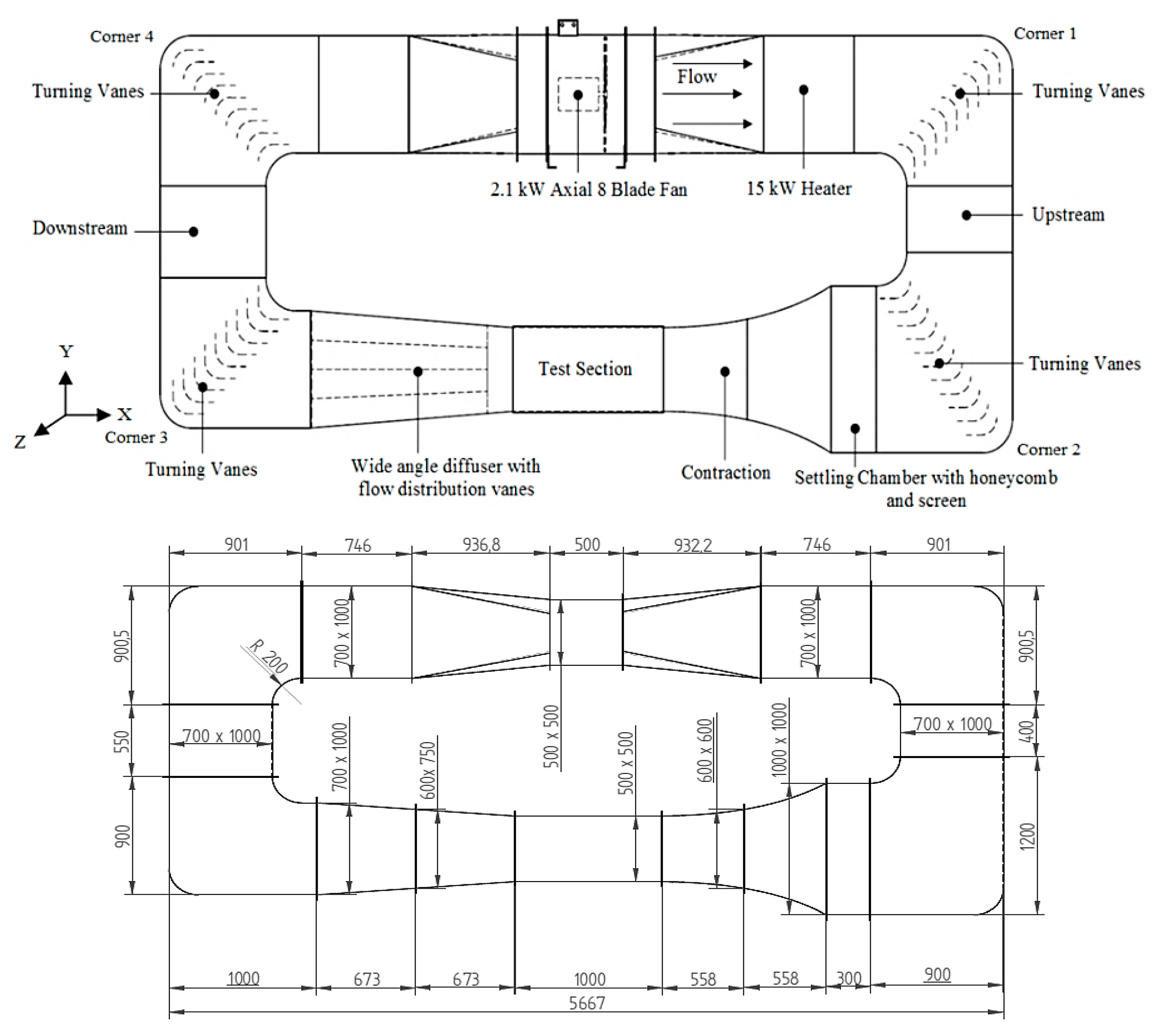
The wind tunnel that was investigated in this study was based on a subsonic closed-loop design built at the School of Civil Engineering at the University of Leeds. The wind tunnel had an overall plan length of 5.6 m with a test section of the height, width, and length of 0.5 m, 0.5 m and 1.0 m, respectively. The tunnel operated as closed circuit in which air that passes through the test section was drawn back into the fan and re-circulated into the test section repeatedly. Guide vanes were used to turn the airflow around the corners of the wind tunnel while minimizing the turbulence and power loss. The contraction, diffuser, test section and two corners were located at floor level while the return legs set with the axial fan were positioned vertically above the test section. The 2.1 kW, 710 mm axial fan delivered the airflow within the test-section which can be varied between 2 m/s and 12 m/s. Controllable heating elements were positioned after the axial fan and prior to the first corner to generate the required air temperatures for experimentation involving temperature variations. The schematic representation of the wind tunnel components and its dimensions are displayed in Figure 1.

Figure 1. Schematic representation of the wind tunnel components.

Figure 1. Schematic representation of the wind tunnel components.

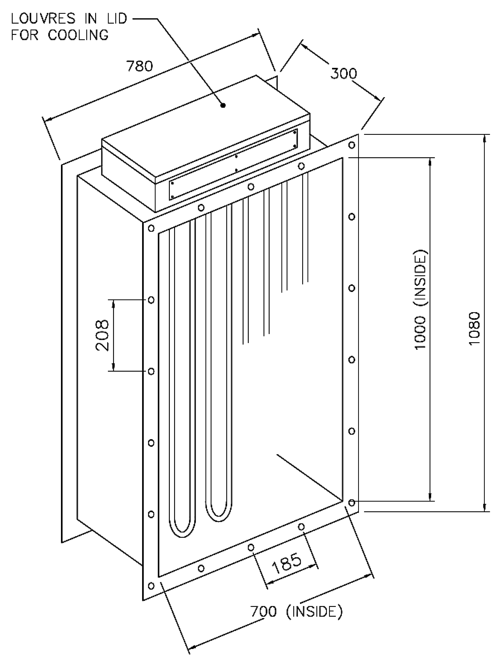
A total of nine heating elements with 10.92 mm diameter (u-bend) were fixed into the 1000 × 700 × 300 mm³ duct using compression fittings (15 KW total) 240 V per element as shown in Figure 2. The control panel was designed to control the operating temperature of a heater. The control panel contained an R38 microprocessor based digital electronic controller, which switched the heater ON and OFF until a preset temperature is achieved. An isolator switch with inlet terminals, power contactor with outlet terminals and J type thermocouple terminal block were fitted and a Miniature Circuit Breaker (MCB) was fitted to protect the control circuit.

Figure 2. Schematic representation of the heating elements inside the duct.

Figure 2. Schematic representation of the heating elements inside the duct.

Table 1. Summary of the design specification and dimensions of wind tunnel components.

Component	Basic Dimensions (mm)	Specification
Test Section	500 (w) × 500 (h) × 1000 (l)	Square cross-section,
Contraction	1000 × 1000 (inlet) / 500 × 500 (outlet)	4:1 ratio
Diffuser	500 × 500 (inlet) / 1000 × 1000 (outlet)	3:1 ratio, 8° conical angles
Round to Rectangle Duct	700 (diameter) / 1000 × 700 (outlet)	Anti-vibration
Settling Chamber	1000 (w) × 1000 (h) × 400 (l)	Honeycomb, wire mesh
Axial Fan	700 (diameter)	2.1 kW

Table 1. Summary of the design specification and dimensions of wind tunnel components.

Component	Basic Dimensions (mm)	Specification
Test Section	500 (w) × 500 (h) × 1000 (l)	Square cross-section,
Contraction	1000 × 1000 (inlet) / 500 × 500 (outlet)	4:1 ratio
Diffuser	500 × 500 (inlet) / 1000 × 1000 (outlet)	3:1 ratio, 8° conical angles
Round to Rectangle Duct	700 (diameter) / 1000 × 700 (outlet)	Anti-vibration
Settling Chamber	1000 (w) × 1000 (h) × 400 (l)	Honeycomb, wire mesh
Axial Fan	700 (diameter)	2.1 kW

The rectangular test-section had cross-sectional area (A) of 0.25 m². The size of the test-section was desirable for the purpose of conducing future experimentation including a greater range of blockage sizes. The hydraulic diameter (D_H) of the test section was 0.5 m. At a temperature of 21 °C and a speed of 10 m/s, the Reynolds Number was calculated at 264 × 10³ while the volume-flow rate (Q) inside the test-section was calculated as 2.28 m³/s indicating a mass flow rate (ṁ) of 2.79 kg/s. The total pressure loss coefficients and head losses were obtained for upstream and downstream wind tunnel sections alongside the corner. The total head loss (H) for the wind tunnel was calculated at 13.35 m providing a total pressure loss of 140.1 Pa [17]. The different sections of the wind tunnel are briefly described by their basic dimensions and specifications. A summary of the design specifications is listed in Table 1.

3. Experimental and Measurement Procedure

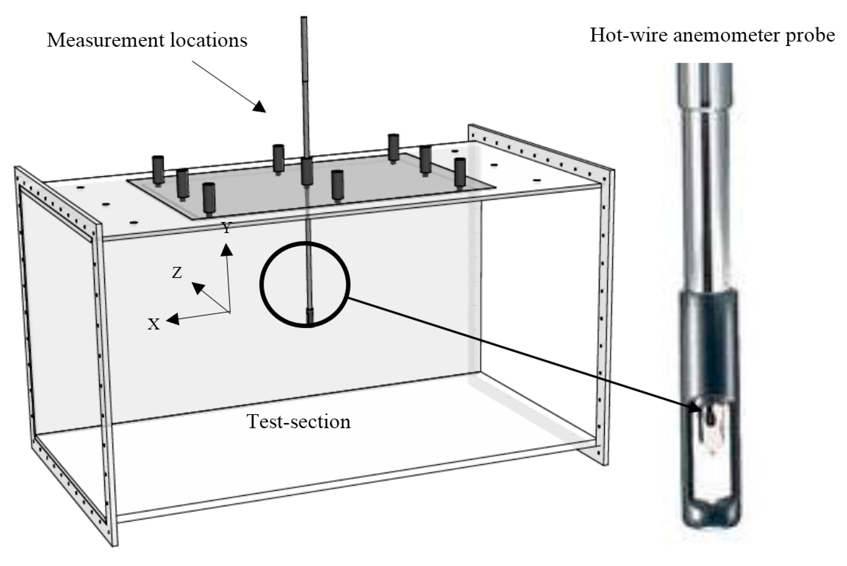
The wind tunnel characterization comprised of measuring air velocity and temperature inside the empty test-section at the designated measuring points. The Testo-425 hot-wire thermal anemometer with a sampling frequency of 1 s was used for this study based on its capacity to measure velocity, temperature and turbulence (Figure 3). The diameter of the probe head was 7.5 mm with a telescoping handle reaching a maximum length of 450 mm. Particular attentions was paid to ensure that the hot wire signal was not contaminated by the temperature fluctuations. Before each measurement, it was ensured that the flow temperature is relatively stabilized and the measurements were compared with a reference thermocouple. In addition, the measurement point closest to the wall was 0.125 m away from the wall and the temperature fluctuation from this region was expected to be significantly lower as compared to the near-wall region.

Figure 3. Schematic representation of the heating elements inside the duct.

Figure 3. Schematic representation of the heating elements inside the duct.

The hot-wire anemometer yielded mean air speed and its time-based equivalent. The average sectional velocity over the local value was used to estimate the non-uniformity “coefficient e” for each point given by Equation (1) [18]:

$$e=\frac{\mathrm{\Delta }u}{\overline{u}}=\frac{u_i-\overline{u}}{\overline{u}}$$

(1)

where $u_i$ represents the actual air velocity at the measurement point i and $\overline{u}$ represents the mean air velocity of all the points.

The non-uniformity and the turbulence level in the test-section were also measured using the hot wire anemometer. It should be noted that measurements were made with single wires, so that the measured turbulence represents only the longitudinal or vertical velocity fluctuations due to the orientation of the wire. The level of turbulence intensity (I) in a wind tunnel can be expressed as a ratio of the standard deviation of the velocity fluctuations to mean stream velocity [19]. The turbulence can be defined as shown in Equation (2):

$$I=\frac{{\sigma }_u}{\overline{u}}$$

(2)

where ${\sigma }_u$ represents the standard deviation of the air velocity and $\overline{u}$ represents the mean air velocity of all the points.

Temperature readings were measured using the Type K Thermocouple (exposed wire, Polytetrafluoroethylene (PTFE) insulated) having a tip diameter of 1.5 mm and a tip temperature range between −75 °C to 250 °C. All thermocouples were calibrated to ±0.1 °C accuracy. The thermocouples were connected to a TC-08 Thermocouple Data Logger, which had a capacity of eight thermocouple channels. The high (20-bit) resolution ensured that the TC-08 could detect minute changes in temperature.

A precise experimental determination of the thermal performance of the test-section requires accurate measurement of the temperatures of the airflow at different locations of the test section, in order to determine the rate of heat transfer across its length. Thermal characterization of the test-section was carried out by averaging the temperature measurements at the respective locations at regular intervals of time. Air density and specific heat capacity values were taken in accordance with the source temperatures. The rate of heat transfer at the test-section of the wind tunnel is formulated using Equation (3):

$$q=\rho UA{C}_{p,G}\left(T_{inlet}-T_{outlet}\right)$$

(3)

where $q$ represents the convective heat transfer of air, U represents the velocity at the measurement location, A is the cross-sectional area and $C_{p,G}$ is the specific heat capacity of air.

Using the controllable motor axial fan, stabilized state and time-based experimentations were conducted at frequencies of 10 Hz, 20 Hz, 30 Hz, 40 Hz and 50 Hz. This was done to have a better understanding of the variation in air velocity at varying inlet fan pressures.

4. Numerical Modeling of the Flow

Following the description of the wind tunnel facility and the experimental method, this section describes the numerical model. The commercial ANSYS Fluent 14.0 numerical code was used for calculating the flow velocity, pressure, turbulence and temperature profiles. A full-scale CFD model of the entire wind tunnel was simulated instead of the conventional approach, in which only the flow in the test section is modeled. The three-dimensional Reynolds-averaged Navier–Stokes (RANS) equations along with the momentum and continuity equations were solved using the commercial CFD code for field simulations. The model employs the control-volume technique and the Semi-Implicit Method for Pressure-Linked Equations (SIMPLEC) velocity-pressure coupling algorithm with the second order upwind discretization as highlighted by Moonen et al. [14].

The standard k-epsilon model [15,17,20] was used for defining the turbulence kinetic energy and dissipation rate within the model. A pressure of 140 Pa was applied at the inlet from the fan in order to overcome the overall loss from the wind tunnel as identified. Standard wall functions were used with a roughness constant (C_KS) of 0.5 applied on the walls. The Quadratic Upstream Interpolation for Convective Kinematics (QUICK) [21] discretization scheme and second-order pressure interpolation was used to achieve higher accuracy of the solutions. For the temperature field, the energy equation was solved in addition to the Navier–Stokes and turbulence equations. Air temperatures of 30 °C (303 K) and 50 °C (323 K) were applied as inlet boundary conditions to the flow. The value for gravitational acceleration was taken as −9.81 m/s² in the Y direction.

4.1. Grid Generation

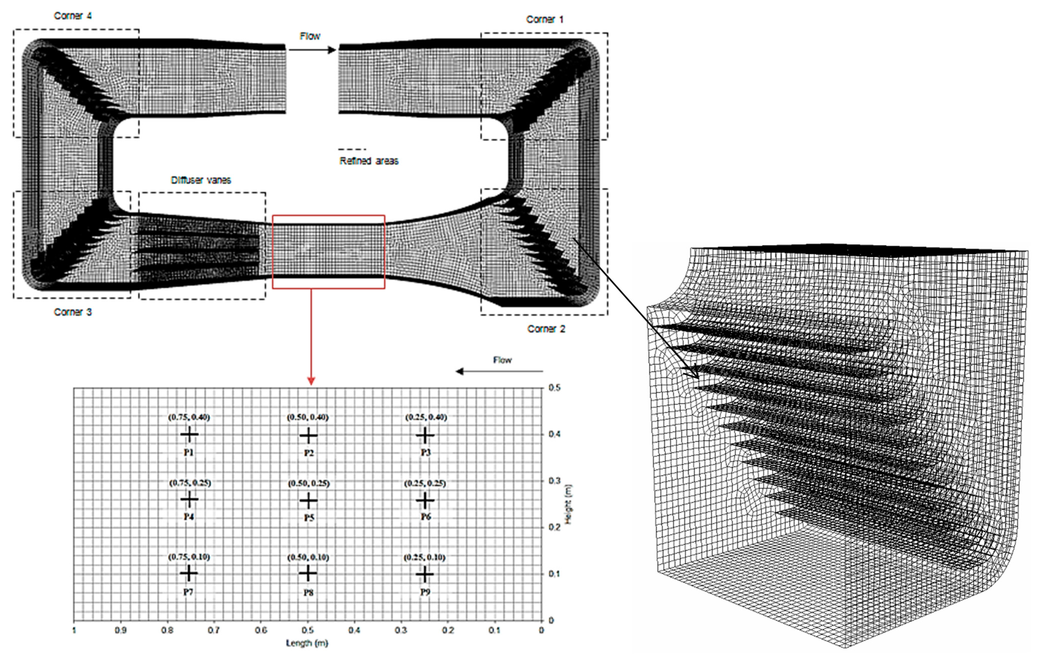
A structured grid was applied on all sections of the geometry [22]. Figure 4 displays the complete meshed model and the co-ordinates of the measurement locations. The complete meshed model comprised of 571,219 nodes and 592,433 elements. Modeling the flow conditions in the entire wind tunnel requires more effort than only modeling the flow in the test section. The grid resolution was determined taking into account an acceptable value of wall y+ (mean value of 290), the cell equiangle skew (average value of 0.1) and the cell equivolume skew (average value of 0.1). A dense mesh resolution was applied at the walls of the turning vanes at all four corners in order to increase the accuracy of capturing the flow passing through.

Figure 4. Grid design highlighting areas of refinements and the measurement locations.

Figure 4. Grid design highlighting areas of refinements and the measurement locations.

As indicated in Figure 4, nine measurement points (P1–P9) across the rectangular cross-section were created running along the entire length of the test-section (between the contraction and the diffuser section), which was 1 m. The points were located to achieve a direct comparison with experimental results. Each point was measured at three different heights, namely 0.125 m, 0.25 m and 0.375 m.

4.2. Grid Validation

The h-adaptivity method described by Chung [21] was used as the grid validation method for this study. In order to verify the numerical models, grid validation was carried out using mesh refinements to optimize the distribution of mesh size (h) over a finite element. In finite element analysis, the basic concept of mesh refinement methods is to refine the element in which a posteriori error indicator is larger than the preset criterion. 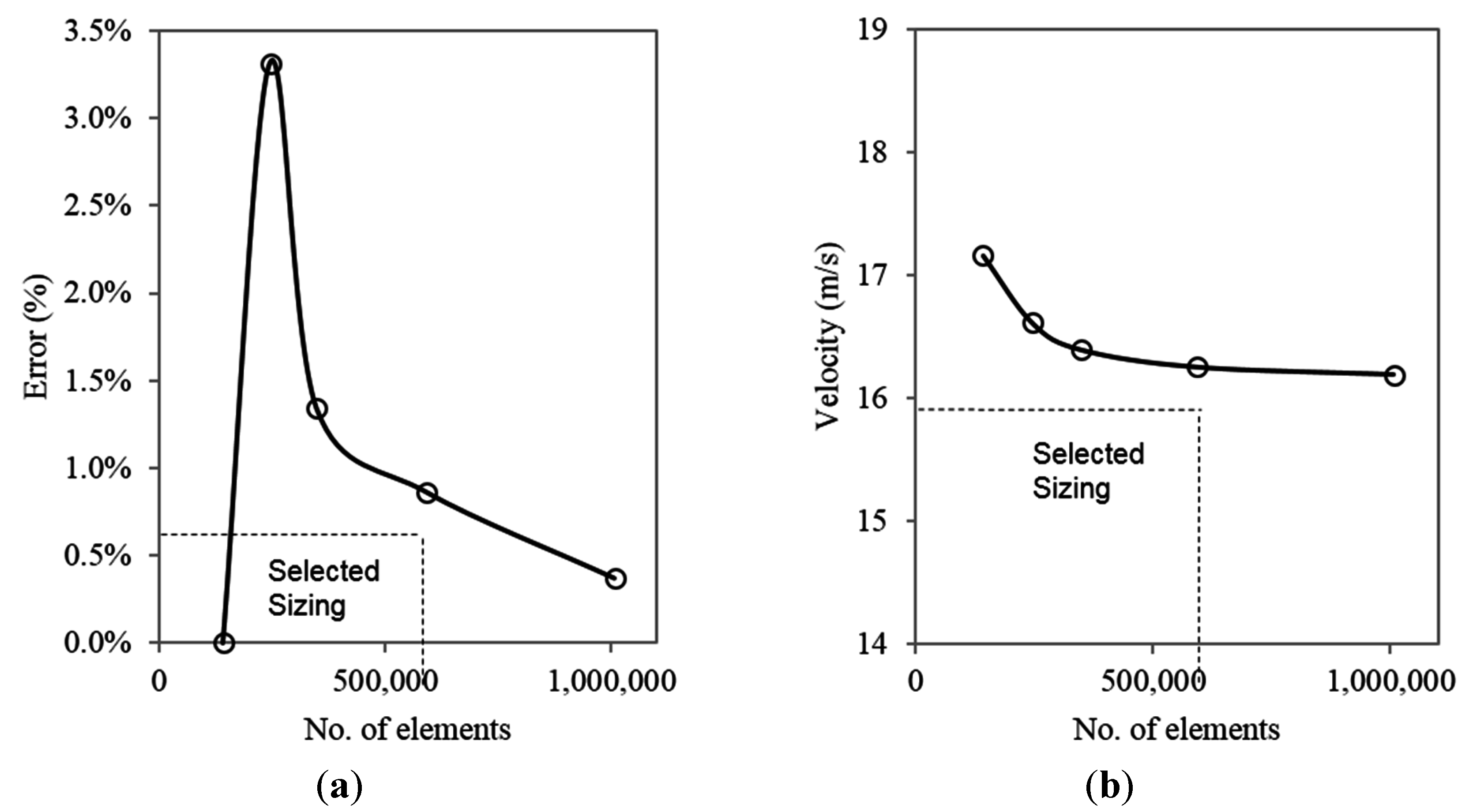To achieve this error estimate, the h-adaptivity method proceeds with an error indicator in terms of changes of gradients of appropriate variables. The mean velocity in the test-section was taken as the error indicator as the grid was refined from 141,500 to 1,007,136 elements. The grid was evaluated and refined until the posterior estimate error became insignificant between the number of elements and the posterior error indicator. The discretization error was found to be the lowest at over one million cells for both indicated variables. In order to achieve a balance between accuracy and computational times, the element sizing of 0.02 was selected.

Figure 5 displays the posterior error percentage for average velocity in the test-section at increasing grid sizes. The maximum error for average velocity was recorded 3.3%. The errors between variables reduced as the grid was refined and dropped to below 1% for average velocity after the element sizing of 0.03 respectively.

Figure 5. (a) Posterior error on the average velocity in the test-section using h-method. (b) Variation in test section velocity at increasing number of elements

Figure 5. (a) Posterior error on the average velocity in the test-section using h-method. (b) Variation in test section velocity at increasing number of elements

5. Results and Discussion

5.1. CFD Predicted Fluid Flow and Temperature Profiles

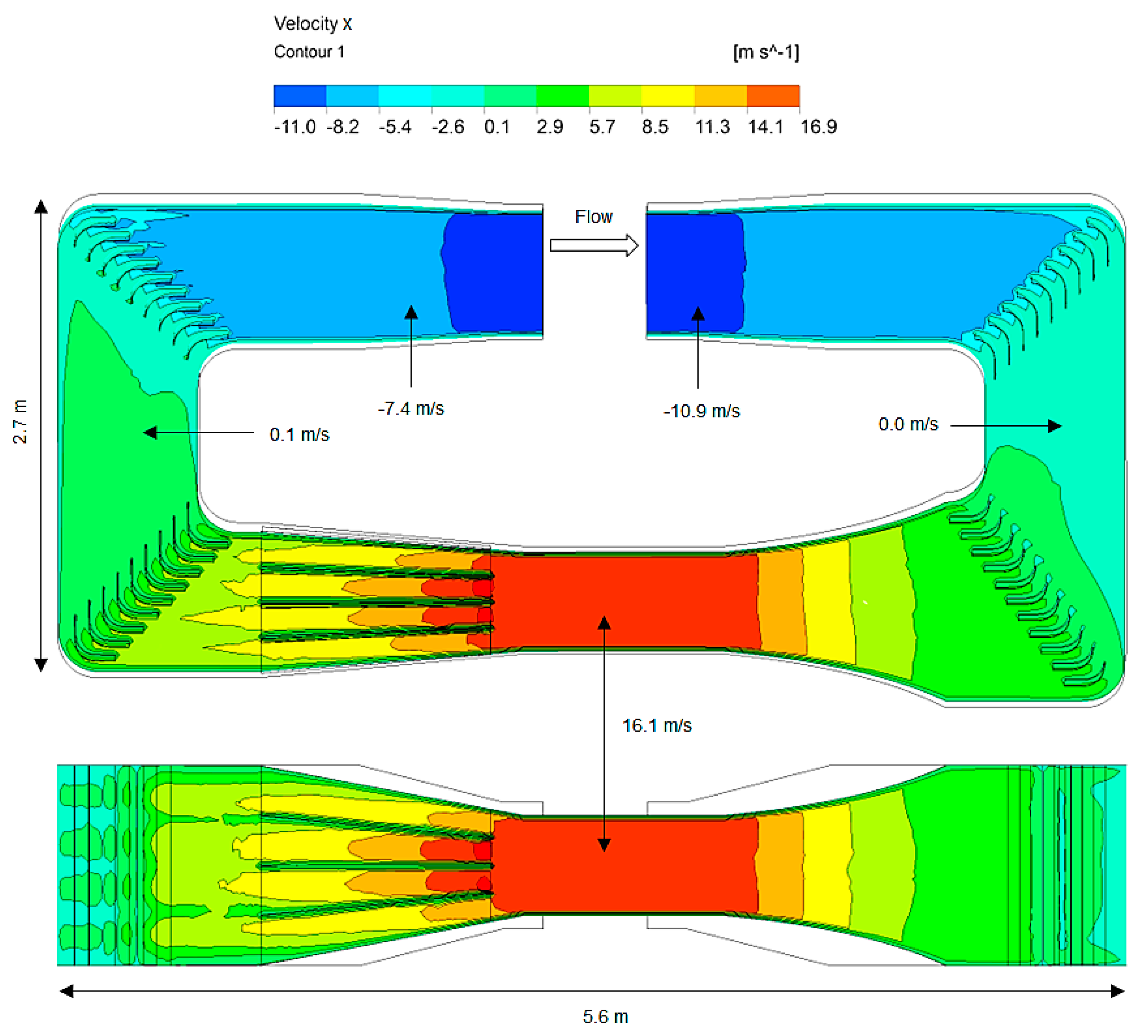
The numerical simulation was carried out on the wind tunnel to determine the flow and thermal profiles. Figure 6 displays the air velocity profile in an empty wind tunnel. At an inlet pressure of 140 Pa from the fan, the mean velocity variation within the test-section was noted to be below 1.5%. The average velocity in the test-section was recorded at 16.1 m/s. An increase in mean velocity from 3.9 m/s to 16.6 m/s was observed from the contraction to the test-section, highlighting an increase factor of approximately four and thereby confirming the correct operation of the contraction section. It was observed that the velocity subsequently reduced as it passed through the guide vanes installed in the diffuser section. The 90° turning vanes located at all four corners aided in reducing the re-circulation of the flow at the bends as there was no velocity rotation in the horizontal axis between corners 1 and 2 and between corners 3 and 4.

Figure 6. Air velocity across the front plane of the wind tunnel.

Figure 6. Air velocity across the front plane of the wind tunnel.

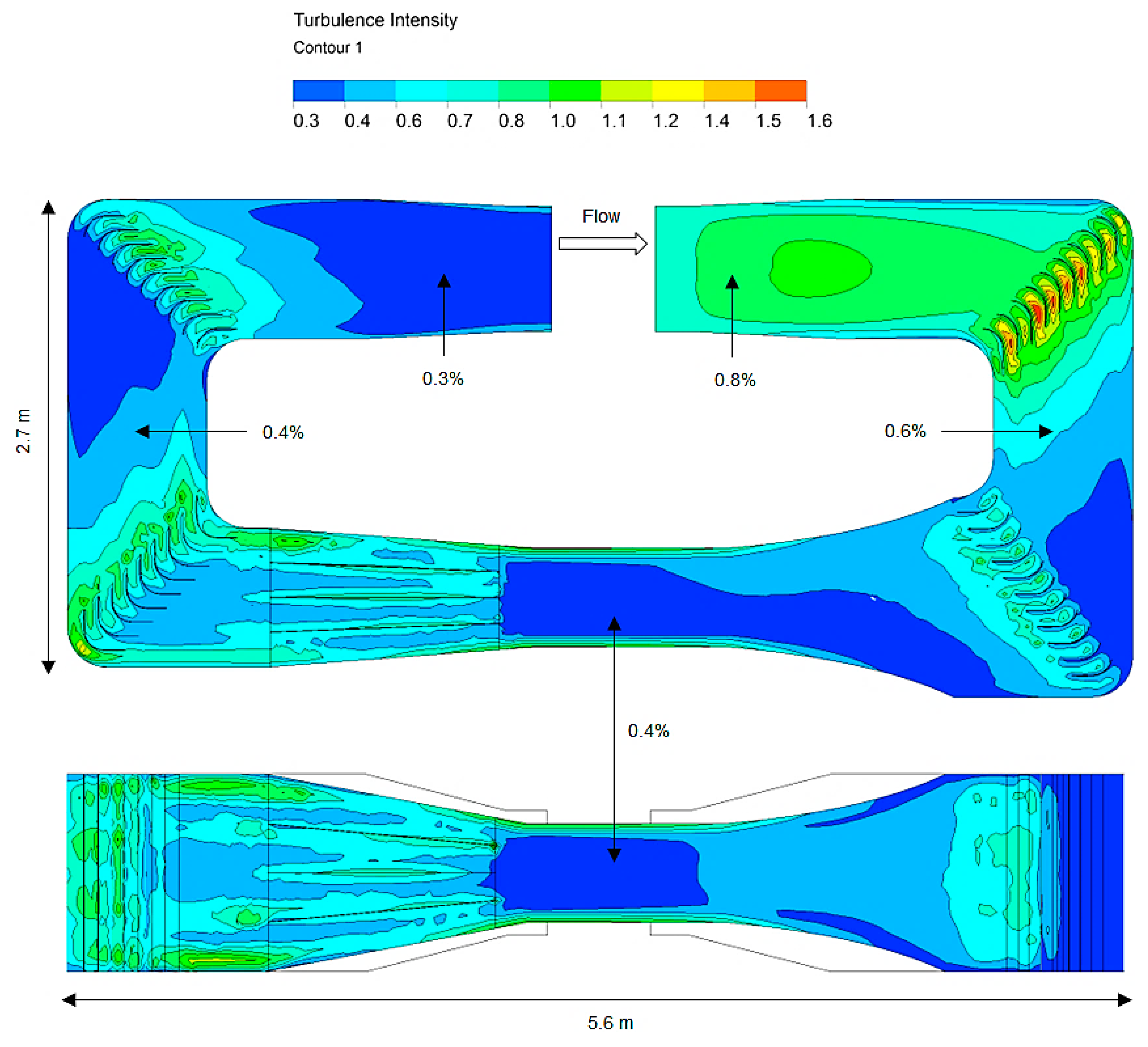
The turbulence intensity across the front plane of the wind tunnel is displayed in Figure 7. The highest region of turbulence was found at the walls of turning vanes in the first corner with the maximum turbulence value recorded at 1.6%. However, the maximum value of turbulence inside the test-section was estimated at approximately 0.5%. The purpose of carrying out the CFD simulations was to ensure accurate flow and turbulence characterization of the wind tunnel prior to the manufacturing process.

Figure 7. Turbulence intensity across the front plane of the wind tunnel.

Figure 7. Turbulence intensity across the front plane of the wind tunnel.

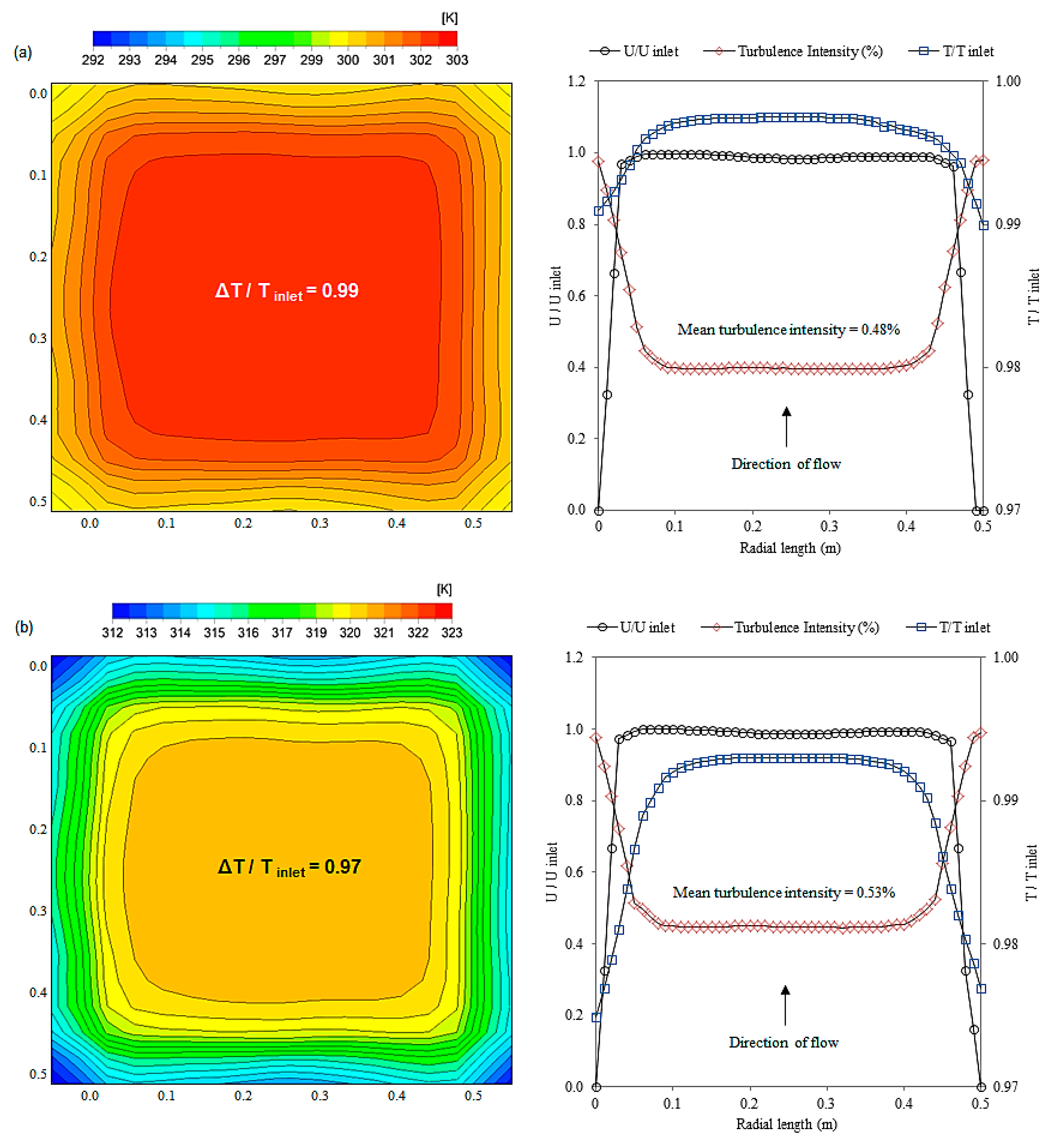
Thermal profiles across the wind tunnel were further determined in order to depict the thermal stratification in the test-section. The inlet temperature in the wind tunnel increased from 293 K up to 323 K. The wall boundary condition was set to non-slip, adiabatic to closely replicate the actual wind tunnel experiment. The temperature flow profile is plotted in Figure 8, highlighting its formation alongside the velocity boundary layer at the two compared temperatures. The numerical simulation showed that the thermal boundary layer thickness was lower when the inlet temperature was 303 K while thermal stratification effects were more significant when the inlet temperature was increased to 323 K. The mean turbulence intensity was determined at 0.48% when the test-section temperature was 303 K. This value was increased to 0.53% when the temperature was raised to 323 K. The relationship between turbulence intensity and temperature is further described in the following section.

5.2. Measured Flow Profiles at Stabilized Operating Temperature

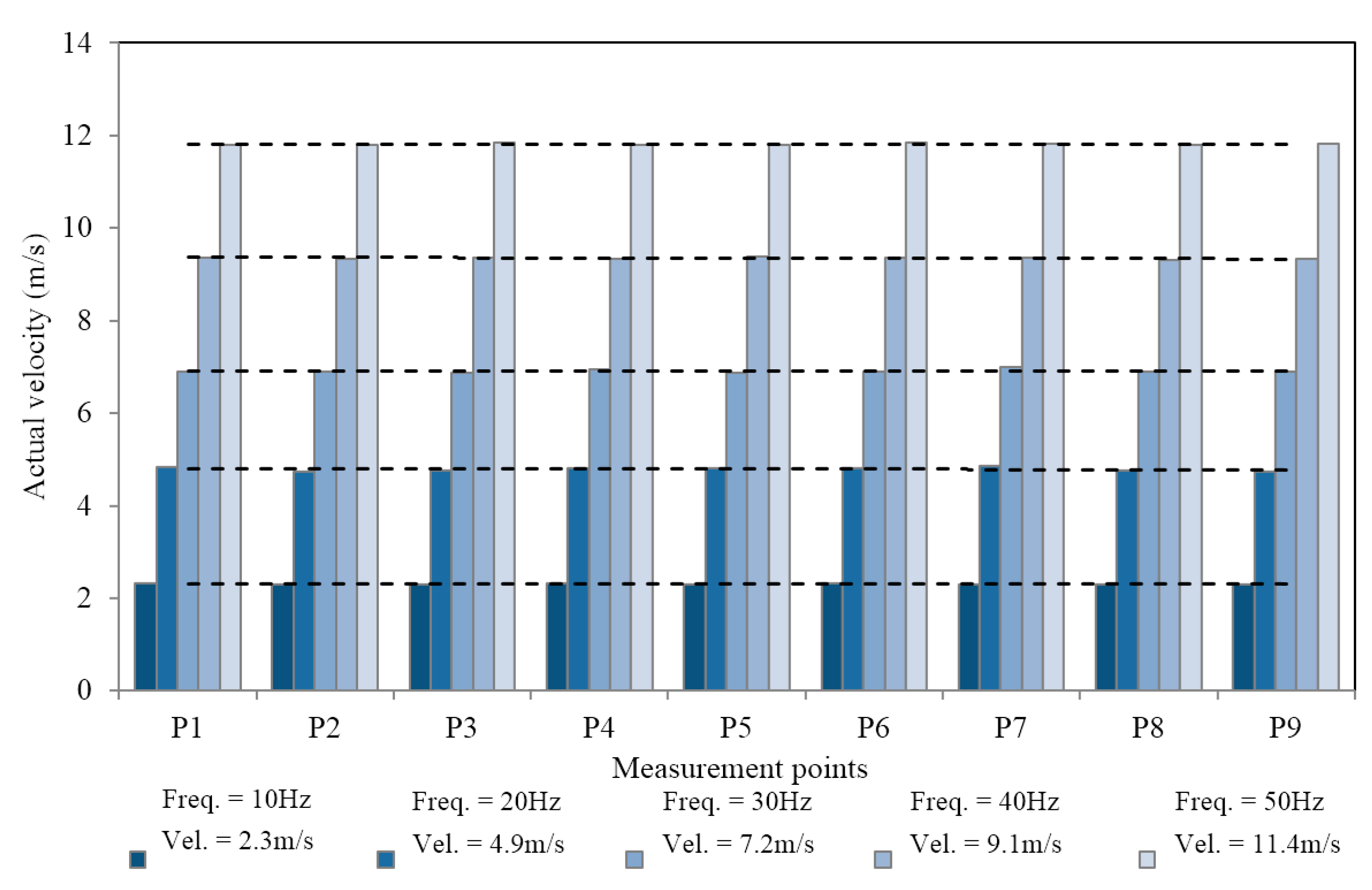
The first phase of experimental testing involved determination of stabilized velocity profiles at fixed inlet temperatures of 20 °C. Testing was conducted at five different fan input frequencies ranging from 10 Hz to 50 Hz. Time based mean equivalent of the velocities were noted at each measuring point and a comparison was established against other points. Figure 9 displays the variation in actual test-section velocity at the measurement locations. The average air velocity is listed below the fan frequency, shown in the figure. A low variation was detected at all measuring points with a mean non-uniformity of 0.9% across all the points in the test section, which is in the recommended range for wind tunnels [18]. At the minimum frequency, the mean non-uniformity was measured at 1.0% and it was observed that the variation reduced as the air velocities were increased. At 50 Hz or the maximum fan frequency, a mean non-uniformity value of 0.7% was measured across the test section.

Figure 8. Temperature, turbulence and velocity distribution in the test-section at (a) 303 K (30 °C ) and (b) 323 K (50 °C).

Figure 8. Temperature, turbulence and velocity distribution in the test-section at (a) 303 K (30 °C ) and (b) 323 K (50 °C).

Figure 9. Velocity profiles in the test section at varying fan frequencies.

Figure 9. Velocity profiles in the test section at varying fan frequencies.

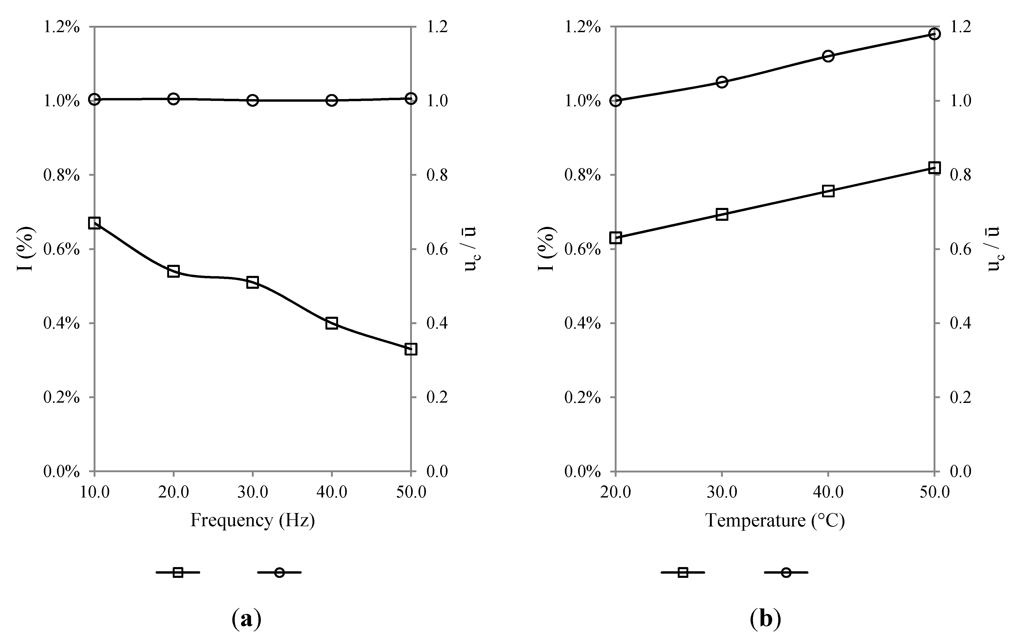
The effects of progressive heating on air velocity were further investigated to determine its impact on non-uniformity and turbulence intensity. Axial velocity measurement (X direction) $\left({\text{u}}_{\text{c}}\right)$ at the centre of the wind tunnel test-section was recorded and a ratio against the mean test-section velocity $\left(\overline{\text{u}}\right)$ was established to highlight the non-uniformity parameter at the point. Figure 10a displays the variation of ${\text{u}}_{\text{c}}/\overline{\text{u}}$ and I (%) against increasing fan frequencies without temperature variation. As observed, the turbulence intensity decreases as the fan frequencies are increased, confirming a superior working performance of the wind tunnel at higher wind speeds.

The ratio of ${\text{u}}_{\text{c}}/\overline{\text{u}}$ remains steady at approximately 1 for all frequencies indicating that the flow variation at the center of test-section remains constant at all equivalent wind speeds. Figure 10b depicts the variations as the operating temperature was increased and as expected, the turbulence intensity percentage was increased by 0.19% as the temperature was increased from 20 °C to 50 °C. This was due to the increasing kinetic energy of the air particles, which increased the corresponding turbulence intensities of the particles [23]. The ratio of ${\text{u}}_{\text{c}}/\overline{\text{u}}$ increased as the velocity values increased from the mean at increasing temperatures to maintain the energy balance of the system.

Keeping a constant operating frequency of 10 Hz, a measurement of mean velocity across the test-section of the wind tunnel was taken at operating temperatures ranging from 20 °C up to 50 °C. This was done to determine the percentage reduction in velocity with the increase in temperature. A steady decrease in velocity was observed as the operating temperatures were increased highlighting an inverse relationship between the two parameters. The total decrease in mean air velocity was 0.36 m/s from 2.37 m/s at 20 °C to 2.01 m/s at 50 °C. As a result, the mean velocity reduction was obtained as 5.1% at 30 °C, which increased to 10.5% at 40 °C and the maximum velocity reduction was observed at 50 °C at 15.2% respectively.

Figure 10. Variation of ${\text{u}}_{\text{c}}/\overline{\text{u}}$ and I(%) at (a) increasing fan frequencies and (b) increasing operating temperatures.

Figure 10. Variation of ${\text{u}}_{\text{c}}/\overline{\text{u}}$ and I(%) at (a) increasing fan frequencies and (b) increasing operating temperatures.

5.3. Measured Flow Profiles at Progressive Increase in Operating Temperature

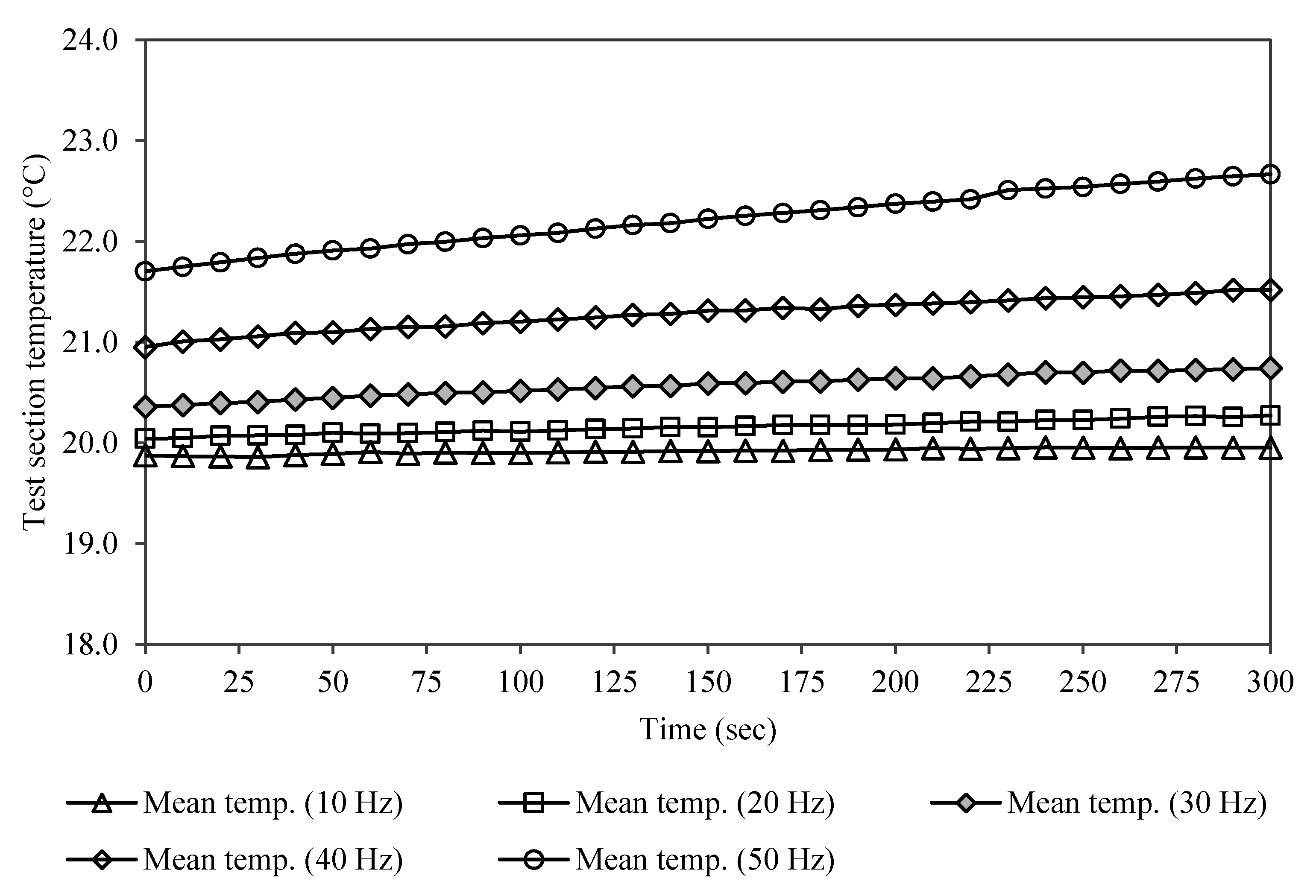
Following the stabilized steady state analyses, a transient test was conducted for better comprehension of the temperature formations inside the wind tunnel. Two sets of experiments were conducted; one with the heating elements turned off and the other with heating elements turned on. The test was conducted at different fan frequencies in order to determine the impact of friction produced by the rotating fan blades on the temperature formations inside the test section. The overall increase in temperature was 2.3 °C after 1500 seconds of run-time. The percentage variation in temperature recorded was the lowest at 0.49% measured at the lowest fan frequency of 10 Hz.

In general, it was observed that both the actual temperature values along with the standard deviation increased as the fan frequency increased. This was expected due to the heat or thermal energy produced by friction from the rotation of the fan blades. The standard deviation (${\text{σ}}_{\text{t}})$ of temperature recorded was maximum at 50 Hz with a value of 0.29, at which the temperature variation was 4.3%. The graphical representation of the results is plotted in Figure 11.

With respect to the heat losses, the average temperature outside the wind tunnel during the duration of the test was recorded at 20.17 °C while the maximum temperature was recorded at 20.25 °C when the heating elements reached their maximum point, thus indicating a differential of 0.08 °C. Using the U value (overall heat transmission coefficient) for the test-section wall surface as 4.9 W/m²K, the heat loss through each wall was calculated at 0.19 W; therefore making the heat losses negligible while the tunnel is in operation.

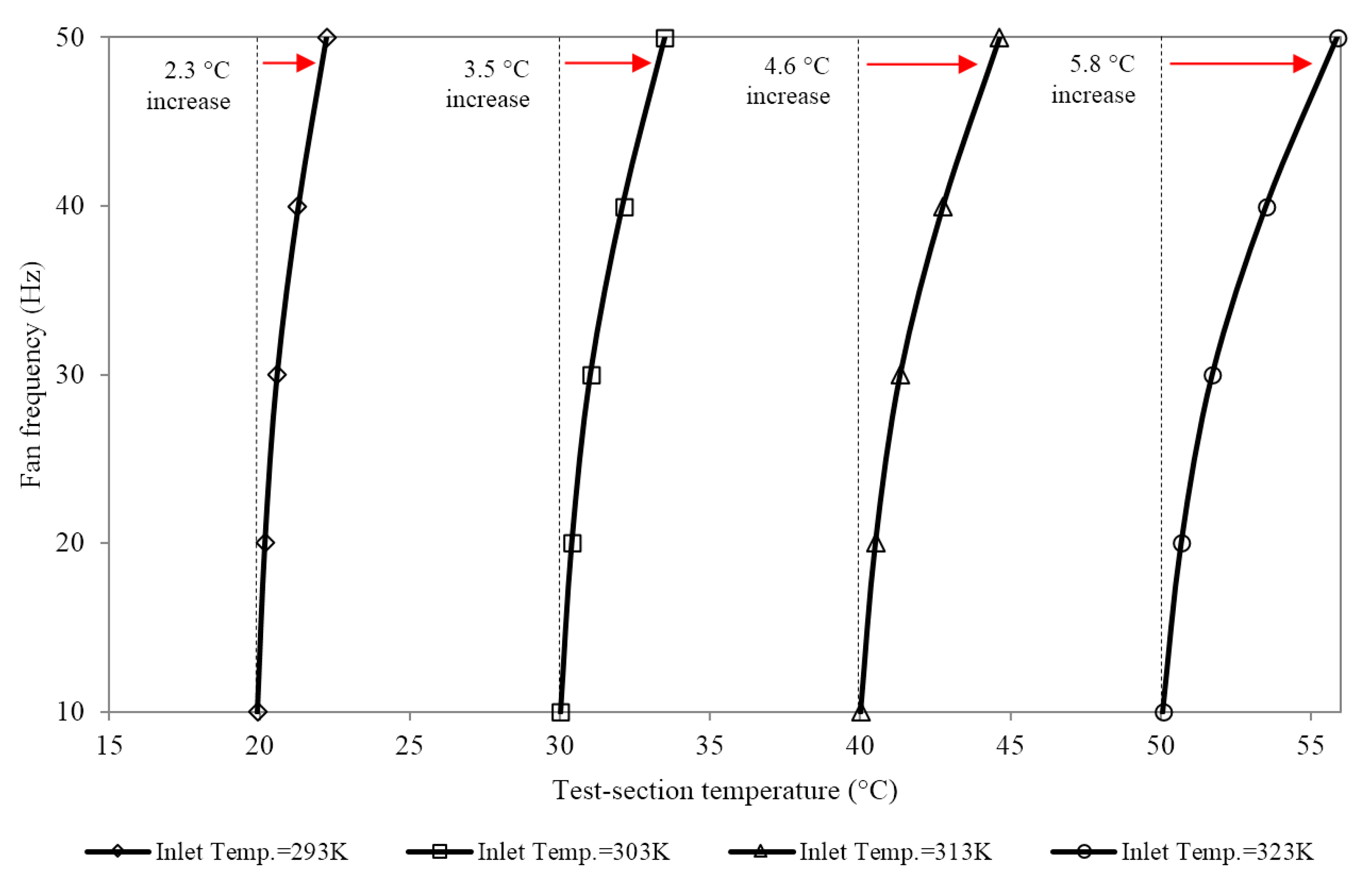
Figure 12 displays the mean operating temperature in the test-section with respect to increasing fan frequencies incremented every 300 s. Due to the friction caused by the heating elements and the fan blades, the operating temperature in the test-section is found to increase with increasing frequencies. An increase of 2.3 °C was observed from the nominal temperature value of 20 °C at a fan frequency of 50 Hz while a larger increase of 5.8 °C was observed from the nominal temperature value of 50 °C at the same frequency. The findings from this investigation thus quantified the effect of progressive heating, both from the fan friction and heating elements on the actual flow and thermal profiles which are expected inside the test section.

Figure 11. Mean test section temperatures at increasing fan frequencies without heating elements.

Figure 11. Mean test section temperatures at increasing fan frequencies without heating elements.

Figure 12. Test-section mean operating temperature at increasing fan frequencies incremented every 300 s.

Figure 12. Test-section mean operating temperature at increasing fan frequencies incremented every 300 s.

6. Validation of Velocity and Temperature Results

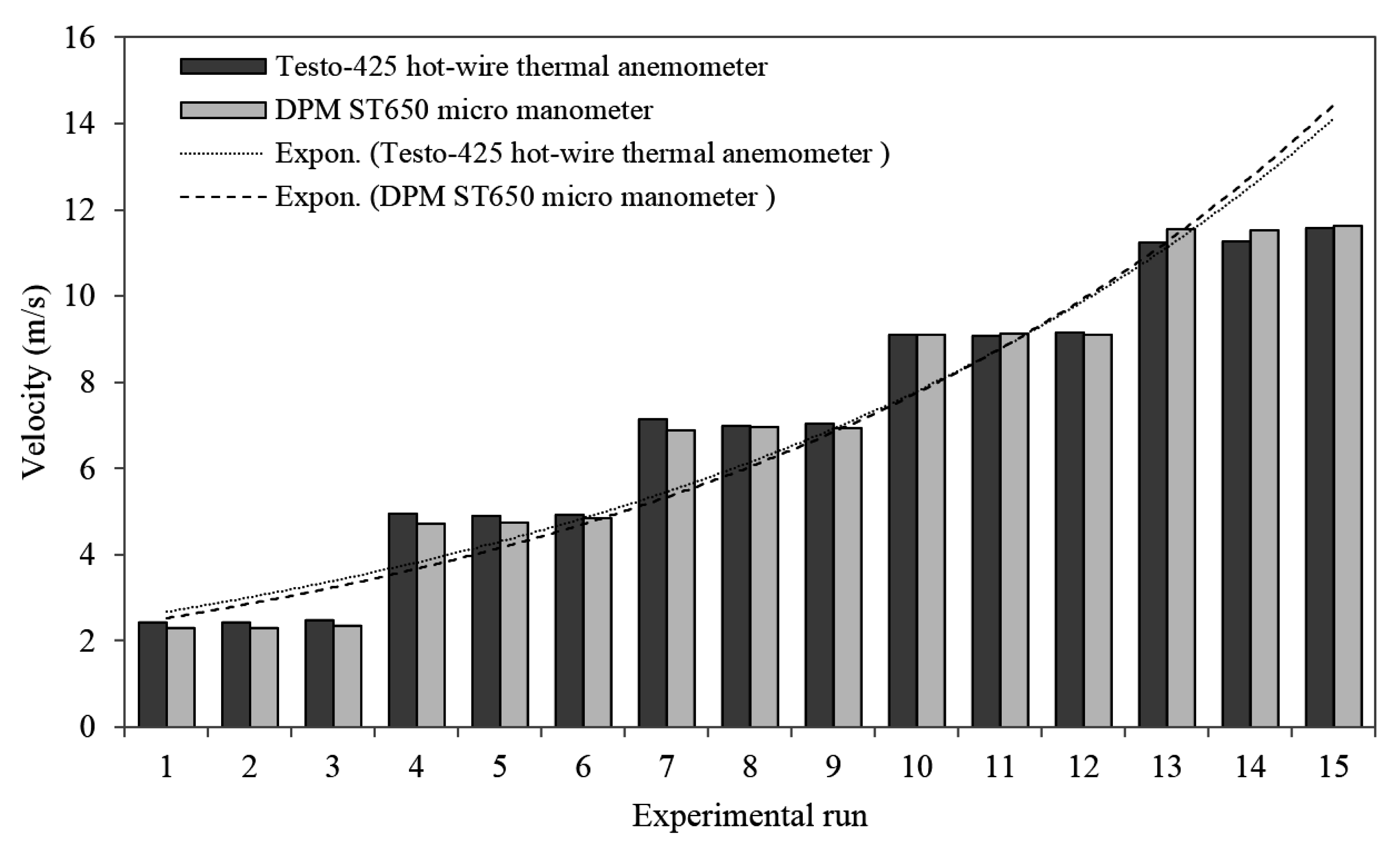
An extensive quantification of the experimental uncertainties was performed in order to determine the accuracy of the measurements. The velocity measurements taken using the Testo-425 hot-wire thermal anemometer were compared against those taken using the DPM ST650 micro manometer. The uncertainty at the test points across the test-section was determined using 15 individual tests at each measurement location. The fan speed parameter was varied after every three tests, ranging from 10 Hz to 50 Hz at increments of 10 Hz. The mean error was calculated at 2.4% across all measurement locations. The maximum error was approximately 5.5% at 10 Hz while the errors were found to decrease at higher fan frequencies. Figure 13 displays the summary of the comparison between the two devices.

Following the uncertainty analysis, the CFD predicted velocity and temperature profiles were validated against experiments based on the located measuring points. The comparison determined the accuracy of the numerical model in relation to the experimental testing. For the velocity parameter, a maximum error of 9.8% was calculated between the CFD and experimental results while the average error percentage was calculated at 6.4%. It was noted that the numerical model under-estimated the velocity non-uniformity and over-estimated the actual velocity values in comparison to the experimental testing. This was due to the numerical model not including the intricate manufacturing joints and fabrication inaccuracies, which were impossible to model prior to manufacture. The variation in velocity using the CFD predicted findings was calculated at 2.5% with a difference of 0.4 m/s between the highest and lowest recorded value. The experimental tests showed lower consistency in results with a variation of 0.9 m/s between the highest and lowest recorded value of the respective.

Figure 13. Comparison of velocity measurements using the Testo-425 hot-wire thermal anemometer and DPM ST650 micro manometer.

Figure 13. Comparison of velocity measurements using the Testo-425 hot-wire thermal anemometer and DPM ST650 micro manometer.

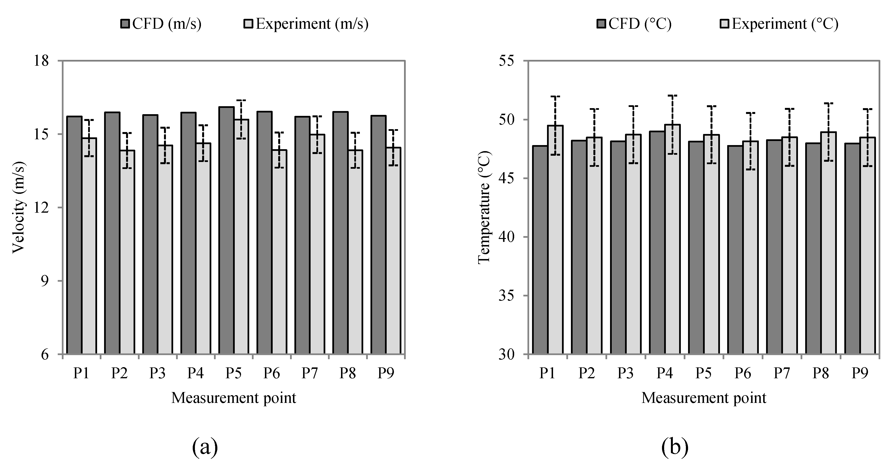
With regards to the temperature parameter, the validation study was performed at the measurement locations set at a fan frequency of 50 Hz. A mean error of 2.3% was obtained between the two compared methodologies. A graphical illustration of the comparison between CFD and experimentally obtained air velocity and air temperature at the measurement points is displayed in Figure 14 with error bars at 5% drawn for the experimental bar for both parameters.

Figure 14. Comparison between Computational Fluid Dynamics (CFD) and experimentally obtained (a) air velocities and (b) temperatures.

Figure 14. Comparison between Computational Fluid Dynamics (CFD) and experimentally obtained (a) air velocities and (b) temperatures.

The good correlation established between the numerically predicted and experimentally tested results identified broad scope for using the advanced computational capabilities of CFD applicable to the thermal modeling of wind tunnels.

7. Conclusions

Flow and thermal characterization of a subsonic closed-loop wind tunnel was carried out using numerical simulation and experimental testing. Based on the overall pressure loss profile, which indicated a loss across of 140 Pa, the mean velocity within the test-section was predicted at 15.7 m/s using the RANS model. Experimental testing was conducted in order to validate the CFD findings at the precise measurement locations. At a constant operating temperature, the mean air velocity depicted from the experimentation was recorded at 14.3 m/s. The validation study therefore indicated a good agreement between the two techniques with a mean error of 6.4%. The experimental results for the test-section velocities indicated a non-uniformity and turbulence intensity of 0.9% and 0.5% across each of the measurement locations in the physical domain. The mean reduction in velocity was 15.2% as the temperature was increased from 20 °C to 50 °C indicating an inverse proportionality between operating velocity and temperature. Thermal stratification effects were influential when the test-section temperature was increased from 20 °C to 50 °C. The present study successfully highlighted the capacity of using CFD and experimental techniques for characterizing the flow, turbulence and temperature profiles within the entire physical domain of a closed-loop wind tunnel.

References

- Mehta, R.D.; Bradshaw, P. Design rules for small low speed wind tunnels. Aeronaut. J. 1979, 83, 443–449. [Google Scholar]
- Cermak, J.E. Wind tunnel design for physical modelling of the atmospheric boundary layer. J. Am. Soc. Civ. Eng. 1981, 107, 623–642. [Google Scholar]
- Mehta, R.D. Turbulent boundary layer perturbed by a screen. AIAA J. 1985, 23, 1335–1342. [Google Scholar] [CrossRef]
- Barlow, J.B.; Rae, W.H.; Pope, A. Low-Speed Wind Tunnel Testing, 3rd ed.; Wiley: Hoboken, NJ, USA, 1999. [Google Scholar]
- Gordon, R.; Imbabi, M.S. CFD simulation and experimental validation of a new closed circuit wind/water tunnel design. J. Fluids Eng. 1998, 120, 311–318. [Google Scholar] [CrossRef]
- Ghani, S.A.A.; Aroussi, A.; Rice, E. Simulation of road vehicle natural environment in a climatic wind tunnel. Simul. Pract. Theor. 2001, 8, 359–375. [Google Scholar] [CrossRef]
- Yassin, M.F. A wind tunnel study on the effect of thermal stability on flow and dispersion of rooftop stack emissions in the near wake of a building. Atmos. Environ. 2013, 65, 89–100. [Google Scholar] [CrossRef]
- Launder, B.; Spalding, D.B. Lectures in Mathematical Models of Turbulence; Academic Press: Waltham, MA, USA, 1972. [Google Scholar]
- Soltani, M.R.; Ghorbanian, K.; Manshadi, M.D. Application of screens and trips in enhancement of flow characteristics in subsonic wind tunnels. Int. J. Sci. Iran. 2010, 17, 1–12. [Google Scholar]
- Manshadi, M.D. The Importance of Turbulence in Assessment of Wind Tunnel Flow Quality. In Wind Tunnels and Experimental Fluid Dynamics Research; InTech: Rijeka, Croatia, 2011. [Google Scholar]
- Cermak, J.E. Wind-tunnel development and trends in applications to civil engineering. J. Wind Eng. Ind. Aerodyn. 2003, 91, 355–370. [Google Scholar] [CrossRef]
- Ohya, Y.; Tatsuno, M.; Nakamura, Y.; Ueda, H. A thermally stratified wind tunnel for environmental flow studies. Atmos. Environ. 1996, 30, 2881–2887. [Google Scholar] [CrossRef]
- Diana, G.; de Ponte, S.; Falco, M.; Zasso, A. A new large wind tunnel for civil-environmental and aeronautical applications. J. Wind Eng. Ind. Aerodyn. 1998, 74, 553–565. [Google Scholar] [CrossRef]
- Moonen, P.; Blocken, B.; Roels, S.; Carmeliet, J. Numerical modeling of the flow conditions in a closed-circuit low-speed wind tunnel. J. Wind Eng. Ind. Aerodyn. 2006, 94, 699–723. [Google Scholar] [CrossRef]
- Moonen, P.; Blocken, B.; Carmeliet, J. Indicators for the evaluation of wind tunnel test section flow quality and application to a numerical closed-circuit wind tunnel. J. Wind Eng. Ind. Aerodyn. 2007, 95, 1289–1314. [Google Scholar] [CrossRef]
- Manshadi, M.D.; Ghorbanian, K.; Soltani, M.R. Experimental study on correlation between turbulence and sound in a subsonic wind tunnel. Acta Mech. Sin. 2010, 26, 531–539. [Google Scholar] [CrossRef]
- Calautit, J.K.; Chaudhry, H.N.; Hughes, B.R.; Sim, L.F. A validated design methodology for a closed-loop subsonic wind tunnel. J. Wind Eng. Ind. Aerodyn. 2014, 125, 180–194. [Google Scholar] [CrossRef]
- Sedov, L.I. Mechanics of Continuous Media; World Scientific: Singapore, Singapore, 1997. [Google Scholar]
- Nader, G.; dos Stantos, C.; Jabardo, P.J.S.; Cardoso, M.; Taira, N.M.; Pereira, M.T. Characterization of low turbulence wind tunnel. In Proceedings of XVIII IMEKO World Congress, Rio De Janeiro, Brazil, 17–22 September 2006.
- Gartmann, A.; Fister, W.; Schwanghart, W.; Müller, M.D. CFD modelling and validation of measured wind field data in portable wind tunnel. Aeol. Res 2011, 3, 315–325. [Google Scholar] [CrossRef]
- Chung, T.J. Computational Fluid Dynamics, 2nd ed.; Cambridge University Press: Cambridge, UK, 2002. [Google Scholar]
- Van Hooff, T.; Blocken, B. Coupled urban wind flow and indoor natural ventilation modelling on a high-resolution grid: A case study for the Amsterdam ArenA stadium. Environ. Model. Softw. 2010, 25, 51–65. [Google Scholar]
- Cochran, B.C. The Influence of Atmospheric Turbulence on the Kinetic Energy Available during Small Wind Turbine Power Performance Testing. In Proceedings of IEA Expert Meeting on Power Performance of Small Wind Turbines Not Connected to The Grid, Soria, Spain, 25–26 April 2002.
© 2015 by the authors; licensee MDPI, Basel, Switzerland. This article is an open access article distributed under the terms and conditions of the Creative Commons Attribution license (http://creativecommons.org/licenses/by/4.0/).