Artificial Immune Classifier Based on ELLipsoidal Regions (AICELL) † †

Intelligent Systems Laboratory, National Technical University of Athens, Athens 15780, Greece
*
Author to whom correspondence should be addressed.
†
This paper is an extended of our paper published in Lanaridis, A.; Stafylopatis, A. An Artificial Immune Classifier Using Pseudo-Ellipsoid Rules. In Proceedings of the 26th International Symposium on Computer and Information Sciences, London, UK, 26–28 September 2011.
Computation 2017, 5(2), 31; https://doi.org/10.3390/computation5020031
Submission received: 31 March 2017
/
Revised: 5 June 2017
/
Accepted: 7 June 2017
/
Published: 17 June 2017
(This article belongs to the Special Issue Computational Aspects Related to Unconventional, Bio-Inspired and Quantum Methods)
Abstract
:Pattern classification is a central problem in machine learning, with a wide array of applications, and rule-based classifiers are one of the most prominent approaches. Among these classifiers, Incremental Rule Learning algorithms combine the advantages of classic Pittsburg and Michigan approaches, while, on the other hand, classifiers using fuzzy membership functions often result in systems with fewer rules and better generalization ability. To discover an optimal set of rules, learning classifier systems have always relied on bio-inspired models, mainly genetic algorithms. In this paper we propose a classification algorithm based on an efficient bio-inspired approach, Artificial Immune Networks. The proposed algorithm encodes the patterns as antigens, and evolves a set of antibodies, representing fuzzy classification rules of ellipsoidal surface, to cover the problem space. The innate immune mechanisms of affinity maturation and diversity preservation are modified and adapted to the classification context, resulting in a classifier that combines the advantages of both incremental rule learning and fuzzy classifier systems. The algorithm is compared to a number of state-of-the-art rule-based classifiers, as well as Support Vector Machines (SVM), producing very satisfying results, particularly in problems with large number of attributes and classes.
1. Introduction
The immune system is a complex of cells, molecules and organs that aim at protecting the host organism from invading pathogens. The system’s ability to recognize these pathogens is not innate, but can be acquired through a complex learning process, which adapts antibodies to recognizing specific types of antigens. However, the invading agents also evolve rapidly, and to combat them effectively the system must be able to generalize its recognition ability to similar, incomplete or corrupt forms of the antigen. In addition to this antigen-specific response, the system must regulate the diversity of its antibody population so that they are able, as a whole, to recognize a wide array of pathogens while, at the same time, not recognize each other, in order to be able to discriminate the pathogens from the organism’s own healthy tissues. These abilities of learning, generalization, noise-tolerance and diversity regulation have made the immune system a suitable source of inspiration for a corresponding bio-inspired model, artificial immune networks.
The response of the immune system is primarily explained by two mechanisms. According to the Clonal Selection [1] principle, when an antigen is encountered antibodies are born to confront it. These antibodies have receptors that adapt their shape through a process similar to natural selection, except on a much faster time scale, in order to better match the corresponding antigen. This evolution is based of a repeated cycle of cloning, mutation and survival of the fittest antibodies, gradually resulting in a population of antibodies of increased ability to match the pathogens, a process known as affinity maturation. The best of these antibodies are stored as memory cells, to be recalled if the antigen is encountered again in the future. Additionally, according to the Immune Network Theory [2], the distinction between antibodies and antigens in not innate to the system. Instead the receptors of antibodies bind to any molecule of matching shape, forming a network of molecules that can recognize, as well as be recognized by, other molecules. To avoid mistaking its own antibodies for pathogens, which results in auto-immune disease, the immune system must ensure that antibodies not only match antigens, but do not match other antibodies. In combination, these two principles mean that the network must evolve in a manner that guarantees both the quality and the diversity of its population. These principles have been successfully applied to the development of engineering approaches, dealing with a variety of classification problems [3], multimodal function optimization [4,5], gene expression tree optimization [6], cascade airfoil optimization [7], breast cancer detection [8] and sensor drift mitigation [9].
We propose in this paper an algorithm applied to one of the central problems of machine learning, that of pattern classification. The proposed classifier encodes the patterns to be recognized as antigens, and evolves a set of antibodies encoding pattern recognition rules of ellipsoidal shape, which are efficient in covering oblique areas of the problem space, in contrast to most rule-based classifiers which are based on rectangular rules. We adapt the innate characteristics of the immune network diversity to ensure the cooperation between those rules, and employ fuzzy membership functions to avoid the exhaustive coverage of the space, which usually results in a large number of rules covering very few patterns, having negative impact on the generalization ability of the classifier. Finally, we modify the computational paradigm, so that the aim of the system is not the recognition, but the elimination of the antigens. This not only brings it closer to the biological model, but also enables us to adapt the fuzzy rules to the approach of Incremental Rule Learning, which combines some of the benefits of traditional Pittsburg and Michigan rule-based classifiers.
A preliminary version of the classifier has been presented in [10]. The current version constitutes a major extension of the former work, including several improvements with respect to both the technical content and the presentation. Among others, a new rule initialization method has been introduced, which, in synergy with the evaluation metric, leads the search to uncovered areas of the problem space, thus improving the performance and convergence of the algorithm. Additionally, the criteria of unfit antibody removal have been extended to include both recognition ability and space coverage. Also, the mutation probability has been adapted to the dimensionality of the problem. Finally, the algorithm has been extensively tested on a number of established benchmark problems, and compared to other state-of-the-art algorithms, using multiple statistical metrics.
The paper continues by giving an overview of learning classifier systems in Section 2. Section 3 provides a description of the modifications made to the immune paradigm and an outline of the proposed method. Individual aspects of the algorithm are discussed in the following sections. In particular, Section 4 describes the form of the classification rule encoded by the antibodies of the network, Section 5 discusses the mutation operator used to evolve it, and Section 6 proposes a fuzzy evaluation metric for selecting the best rules. A suitable rule initialization process is described in Section 7 and Section 8 discusses the preservation of the network quality and diversity by removing unfit antibodies. Section 9 sums up the previous sections in a formal description of the algorithm, and the paper concludes with Section 10, which tests the proposed algorithm on a set of benchmark problems, compares it against state-of-the-art algorithms, and applies a number of significance tests to assess the results.
2. Overview of Learning Classifier Systems
Pattern classification aims at finding a function that maps a vector describing the features of a pattern to a category among a given set. The problem is approached in various ways, with some algorithms assigning the pattern to the class having the most similar patterns (a typical example being k-nearest neighbors algorithm), while others classify it based on some statistical attributes of the patterns in each class (the most well-known example being Naive Bayes Classifier). However, most algorithms approach the problem in a geometric manner, searching the vector space for hyper-surfaces that separate patterns of different classes. Typical examples of this approach are Support Vector Machines (SVM) and Neural Networks.
Another popular type of geometric classifiers are decision trees, which partition recursively each attribute’s range of values into subranges, until a stopping criterion is met. In this manner, decision trees separate the problem space into subspaces, each described by a rule of the form if and then class. Although all geometric classifiers form a set of rules mapping a pattern to a subset of the problem space, rules of this particular form are easily interpretable, and for this reason, decision trees are often called rule-based classifiers.
However, finding the optimal set of such rules is an NP-complete problem [11], regardless of the optimality criterion used. As as result, most rule-based classifiers rely on greedy algorithms that partition the space iteratively, with the aim of maximizing some separation criterion, with information gain being the most common. The use of evolutionary algorithms was proposed by Holland [12] as an alternative, leading to learning classifier systems. To implement a such system, two important decisions have to be made, namely, how the chromosomes represent classification rules, and how the evolutionary algorithm is used to evolve them. Traditionally, there have been two main approaches (see [13] for details).
According to the Pittsburg approach [14], a chromosome encodes a set of rules forming a complete classifier. The genetic algorithm applies crossover and mutation to the best of these rules. Since each chromosome represents a complete classifier, evaluation is straight-forward. However, chromosomes tend to be long, making the search space too large. Morever, either the number of rules has to be decided in advance, or some variable-length mechanisms have to be employed, making optimization even harder. According to the alternative Michigan approach [15], each chromosome represents an invidividual rule, resulting in much smaller search space, and easier optimization. However, evalution of the rules becomes much more complicated, since they have to be evaluted both individually, as well as in terms of their ability to co-operate, to form a complete classifier.
As a compromise between the two approaches, Incremental Rule Learning [16] algorithms were proposed. According to this approach, each chromosome encodes a single rule, as in Michigan classifiers. However, instead of evolving the complete set of chromosomes simultaneously, the algorithm begins with an empty set and adds a new rule at each iteration. Each rule evolves individually, while patterns that are covered by existing rules are removed from the dataset, to avoid overlap and ensure that newly-created rules search uncovered areas of the problem space. To a large extent, this approach combines the smaller search space of Michigan and cooperation of Pittsburg classifiers.
Regardless of which of the above approaches is followed, there is a number of additional implementation choices which have an important effect on the resulting algorithm.
- If the classifier rules are ordered, they form an if-elseif-else chain, and the pattern can be assigned to the first rule whose condition is satisfied. However, with unordered rules of if-else form, further actions are needed to ensure their co-operation, minimize the overlap, and assign the pattern to a class.
- The most common form of condition combines clauses of the form for each dimension of the problem. These rules form a hyper-rectangle, whose faces are parallel to the axes. However, by using a linear combination of the pattern attributes, oblique areas of the problem space can be covered. These linear rules can be combined to form surfaces of arbitrary shape. Alternatively, inherently non-linear rules can be used, such as spheres, quadratic or ellipsoidal surfaces.
- If the patterns are presented to the classifier one at a time, the fitness of the rules that recognize the pattern increases, while for the others it decreases. If no rule matches the pattern, a new one is created. When the patterns are presented in batch, the algorithm can focus of the total coverage of the dataset by the existing set of rules.
- The rules must be evaluated both individually and as a whole. The individual evaluation can be based on either the rule’s ability to accumulate high reward values (strength-based) or its ability to predict its reward, regardless of its value (accuracy-based). To evaluate the rule-set as a whole, various criteria can be used, regarding the total coverage of patterns, minization of overlap, fitness sharing, etc.
- Most of the rule-based classifiers rely on crisp memberhip functions. To cover all the patterns of the dataset, they often have to create rules covering very few patterns, with low generalization ability. The employment of fuzzy membership functions resolves this problem to some extent, but is not consistent with most existing evaluation criteria.
3. Outline of the Immune Network Classifier
Based on the biological principles of affinity maturation and immune network theory mentioned in Section 1, a multitude of computational models have been developed (we refer the reader to [17,18,19] for an extended overview). While each model differentiates from the others in specific aspects, all of them have in common the fact that they address the problem by maintaining a population of antibodies. These antibodies construct a network in the sense that they perform a task in collaboration (while each single member of the network is incapable of producing results), and that the evolution of each antibody depends on specific qualities of other antibodies present in the network. The evolution of each individual antibody is based on criteria concerning its quality, while the evolution of the network as a whole is based on the preservation of diversity, by removing antibodies that are too similar and replacing them by new ones.
Throughout the evolution of the network, antibodies are born, evolve and die. In particular, new antibodies are born when the size of the population is insufficient to confront the antigens. On the contrary, when the population size increases beyond the desired size, the antibodies that do not considerably contribute to the diversity of the network die, leaving space for the fittest and most diverse antibodies to evolve. Antibodies that both exhibit sufficient quality and contribute to the diversity remain in the network. The evolution of these antibodies is based on the clonal selection principle. That is, for each antibody a number of clones (exact copies of the antibody) are created, and the clones go through a mutation process, producing variants of the original antibody. Among these variants, the best ones survive and are inserted to the network.
However, contrary to the computational models, the aim of the biological immune system is not the recognition, but the elimination of the antigens. The recognition ability acquired is a by-product of this process. The suggested algorithm follows this approach which, not only brings it closer to the biological model, but also yields practical benefits, as shown in the following sections. To incorporate that into the algorithm, we introduce a health factor for each antigen, described by a variable . The use of the term health does not imply that the antigen is beneficial to the organism, but quantifies the degree to which it can withstand the damage inflicted by the antibodies before it is dead. This factor is also an indicator of the strengh of the antigen, and consequently the importance assigned to it by the network.
Each of the antibodies composing the network is dedicated to a particular class of antigens. The antibody weakens the antigens of that class to a degree proportional to its affinity to them, having no effect on antigens of other classes. Consequently, the throughout the individual evolution of a rule, the antibody aims at maximizing its affinity to antigens of the same class. The overall evolution of the network is based on the creation and addition of such rules. If the addition of new antibodies results in large degree of similarity or some antibodies presenting lower-than-average recognition ability, these antibodies die and are removed from the network. At each point, the overall effect of the network to an antigen is proportionate to its total affinity to all the antibodies of the same category in the network. The process continues with the addition of new rules, until all antigens are dead or sufficiently weakened.
For the purpose of pattern classification, each antigen encodes a pattern to be recognized, along with its class, and antibodies encode recognition rules. The following chapters explain in detail the form of these rules, the mutation and evaluation process, and the preservation of network quality and diversity by removing unfit antibodies. The combination of these elements results in the proposed system being a strengh-based, fuzzy incremental rule learning classifier.
4. Rule Encoding
In constrast to most rule-based classifiers, which encode rules having an if and then class form, producing hyper-rectangles in the problem space, the proposed method employs rules of ellipsoidal form. Such rules have been used in some cases in learning rule systems [20,21,22,23]. However, ellipsoidal surfaces are computationally complex, and all of the above algorithms rely on some clustering method to decide the number and center of the ellipsoids in advance, while the evolutionary algorithm is used for micro-tuning of the parameters.
On the contrary, the proposed method is a complete algorithm of producing a set of fuzzy rules based on ellipsoidal surfaces. The system evolves such rules dynamically, defining their number so that they cover all of the dataset, while at the same time, not being too similar or having too much deviation in terms of their quality. To simplify the computations, an alternative form of the ellipsoid is used, which, although not completely equivalent, retains its basic characteristics.
4.1. Ellipsoid Definition
An ellipse is the locus of the points on a plane for which the sum of distances to two constant points focal points is constant, that is, the set of all x for which
The above locus can also be generated by the linear transform of a circle. As a result, an ellipse can be equivalently defined as
where A is a matrix representing a linear transform (scaling and rotation), b is the translation from the origin of the axes, and is the unit circle centered at the origin, producing the equivalent definition
where is a symmetric, positive-definite matrix.
If Equation (3) is used to create a set of points in a 3-dimensional space, the resulting locus has the property that its intersection with every plane that passes through point b forms an ellipse. In this sense, it can be regarded as a 3-dimensional equivalent of the ellipse, which is called ellipsoid. Althrough this definition concerns only the 3-dimensional space, similar sets of points in higher dimensions are often also called ellipsoids.
The set of points produced using Equation (1) in 3 dimensions does not have this property, which characterises an ellipsoid in the strict sense. Still, it produces a quadratic surface whose points have the same total distance to two other constant points in that space. In this sense it forms a 3-dimensional generalization of the ellipse, and is used in the current algorithm as the basis for recognition rules. This form constitutes a broad-sense formulation of the ellipsoid, which retains the essential geometric characteristics of the ellipse, while also being significantly simpler computationally than the form described by Equation (3).
4.2. Fuzzy Pseudo-Ellipsoidal Rules
To produce the classification rule, we first re-write Equation (1) as
which re-defines the ellipsoid as the set of points x for which , regardless of the size of the ellipsoid.
However, all of the above equations describe an -dimensional closed surface in the n-dimensional vector space. Given that this surface is intended to be used as a classification rule, we are concerned not only with the points on the surface, but also with the ones inside the enclosed volume. This set of points consists of the points for which . Equivalently, we could define the volume enclosed by the ellipsoid, as a membership function given by
where is the normalized distance of a point x from the two focal points, as defined by Equation (4).
This crisp membership function partitions the space into points inside or outside the space enclosed by the rule. To create a fuzzy rule, this membership function must be transformed to a fuzzy one, so that every point belongs to the rule to some degree. For this purpose, we use the function
where is a parameter defining the steepness of the membership function. It can be seen that for the above equation reduces to (5). In practice, a typical range for the values of f is , since for lower values the function becomes almost uniform, while for larger ones it closely resembles the crisp membership function.
5. Mutation Operator
Given the critical role of mutation on the evolution of the network, this section provides a detailed description. We first describe the operator used, specifically the non-uniform mutation operator for real-valued features, defined in [24]. After that, we adapt the mutation range of each feature to the particular characteristics of the proposed rule form, and the mutation probability to achieve its most efficient performance.
5.1. Non-Uniform Mutation Operator
Given a vector to be mutated, the non-uniform mutation operator acts on each of its attributes with probability . Assuming an attribute selected for mutation, the operator produces a new value
where
In the above equations, and are random values drawn from the standard normal distribution . The quantity defines the range of the mutation, which is a function of the current generation t. For the operator to function properly, the value must be confined in and its value must decrease as t increases. Given a such , the function returns a value in such that the probability that increases as t increases. As a result, as the training progresses, the produced value will be closer to the initial value . This property allows the operator to search the problem space globally at first and more locally in later stages of the training.
The originally proposed form of , which is also used here, is
where t is the current generation of the training, T is the total number of generations, and b a parameter defining the decay of with t. This form has been widely employed in the literature, with typical values of b lying in .
5.2. Mutation Range
For the non-uniform mutation to function properly, each attribute x must be confined in a range . To simplify the procedure, all the patterns of the dataset are normalized so that all the values of their attributes lie in . After the normalization, all the attributes of the vectors describing the focal points of the ellipse also lie in , and can take any value in that range.
On the contrary, the distance r of the surface of the ellipsoid from the focal points can not take any value. Its minimum value must be at least equal to the distance between the focal points, that is
Regarding its maximum value, there is no constraint. However, is should be large enough so that it can cover the whole problem space. As such value, we choose the largest possible distance in that space, that is
where n the number of dimensions.
However, the interval cannot be use directly as mutation range for the attribute r, since the value of changes every time the focal points are mutated. For this reason we define a factor , which is used for linear mapping from to the current value of . The mutation operator is applied to this quantity, and after the mutation of and the evaluation of the resulting , the value of r is calculated by
Finally, the shape of the membership function relies on f. For the function becomes almost uniform, while for the function resembles the crisp membership. To avoid these extremes, it is confined in , where the values are selected experimentally (with a typical value range being ) .
5.3. Mutation Probability
A central characteristic of genetic algorithms is that they rely mostly on crossover to evolve the population of candidate solutions [12,25]. Very few members of the population are selected for mutation and, when this happens, it is usually to introduce diversity in the population. For this reason, the algorithms employing mutation usually mutate all the attributes of the solutions. The resulting solution is usually far from optimal, but that is not a concern, because it will be improved with the crossover operator. On the contrary however, immune systems rely solely on mutation to evolve the population, and consequently a different strategy must be used.
The mutation of an attribute of a candidate solution is a random procedure and, as such, it can be beneficial or detrimental to the quality of the individual. When the number of attributes selected for mutation is small, the probability that all, or most or the mutations are beneficial is significant. However, as the number of selected attributes increases, this probability decreases dramatically, and reduces to random search for a large number of mutated attributes.
For this reason, we select a number of attributes to be mutated at each generation, and, if n is the total number of attributes composing each solution, the mutation probability of each attribute is set to
It is noted that this probability concerns only the focal points of the pseudo-ellipsoid. The quantities and f are scalar quantities, and are mutated in every generation of the training.
6. Evaluation Metrics
In this section we give a brief description of some commonly used rule evaluation metrics (we refer the reader to [26,27,28] for more details), and provide a modified evaluation metric for the proposed fuzzy classifier.
6.1. Common Evaluation Metrics
With the exception of Pittsburg classifiers, all learning systems rely on a criterion that evaluates rules individually. Most criteria are based on the common precision and accuracy metrics. Assuming that is the total number of positive and negative patterns in the dataset, and the number of positive and negative patterns covered by a rule, accuracy is defined as
This equation can be reduced to , where are two constants. Consequently, the main characteristic of this rule is that it assigns equal importance to covering a positive and not covering a negative pattern. As a result, rules covering many patterns can receive a high accuracy score, even if they include a large number of negative patterns, reducing the percentage of correct classifications.
Precision is defined as
This quantity evaluates the percentage of correct classifications, but completely ignores the size of the rule, often producing too many rules covering a small number of patterns. Such rules, despite covering only positive patterns, have little or no generalization ability.
As a compromise between the two criteria, the m-estimate has been proposed
This quantity is a modification of precision, requiring that each rules covers at least m patterns. The value of m decides the trade-off between classification percentage and size of the rules, as it is obvious that for it converges to precision, while it can be shown that for it converges to accuracy.
6.2. Fuzzy m-Estimate
The evaluation metric defined by Equation (16) relies on the number of patterns covered by a rule. However, the proposed method uses fuzzy rules, and so every pattern in the dataset is covered by every rule to some degree. As this degree is quantified by the value of the membership function, we can regard the fuzzy equivalent of as
where is the membership of the i-th antigen to the rule.
Moreover, the algorithm assigns to each pattern importance proportional to the strengh of the antigen that encodes it. Given that this value is given by for the i-th pattern, the above quantities have to be further modified by weighting the patterns by that quantity, resulting in
This modification ensures that the network assigns maximum importance to stronger antigens (), while weak or dead () antigens have little or no effect to the evolution of the rule. From an algorithmic point of view, this weight factor leads the search of the space to areas that have not yet been covered sufficiently by existing rules, since in already covered areas and the value of the evaluation metric will be small, while in uncovered areas and the metric receives larger values.
By replacing these terms in the original equation, the evaluation metric becomes
This modified criterion combines the original m-estimate with the fuzzy membership function, and makes the proposed method a fuzzy generalization of the Incremental Rule Learning strategy. In particular, as the steepness of the membership function increases to , the value of the membership function converges to , and the health of antigens covered by the rule to . Since the contribution of these patterns to Equation (19) reduces to 0, these patterns can be regarded as effectively removed from the dataset, and the behavior of the algorithm converges to that of a standard Incremental Rule Learning system.
7. Rule Initialization
In traditional learning classifier systems, the rules are randomly initialized [12,14,15], and it is left to the evolution process to lead them to the appropriate areas of the problem space. The same approach can be followed in the proposed system. However, given that the purpose of the training is to cover the problem space to the largest possible extent, it is preferable that the new rules are created in areas that have not been already covered. In our case, these areas are the ones where health h of the antigens has high values.
To detect such areas, each time a new rule is to be created, all the patterns of the dataset are examined as candidate centers of the rule. For each pattern, its nearest neighbors are detected, and the sum of their values is calculated. We note that in this calculation, only the patterns belonging to the same class as the candidate center are included. The value of the sum is given by
The area where has the maximum value is the one that has been covered to the least degree up to that point, and the most suitable for a new rule. However, it is not guaranteed that this rule will have a sufficient fitness value. In this case, the produced rule will be removed, and the system will create a new one. Since the removed rule has no effect on the antigens, if the selection was deterministic, the same rule would be created again, resulting in an endless loop.
To avoid this, the pattern that will be the center of the new rule is not chosen deterministically according to the value , but instead, by using tournament selection. Each pattern can be selected with probability
where c is such that
Consequently, the selection probability of the i-th pattern is
The above procedure selects the center of a new rule to be created. We note that, since the network is based on ellipsoid rules, each rule has two focal points. Consequently, during the initialization, the two points coincide, since they are given the same initial value. However, this has no effect on the evolution of the rule, since they will be differentiated when the training begins, due to the mutation operator.
The suggested initialization method has a significant impact on the performance of the algorithm. Figure 1 gives an illustrative example, comparing the decay of the average antigen health during the incremental addition of 50 rules, for 3 executions of the algorithm, for both initialization methods. The results shown regard the libra dataset (which will be presented in the experimental section), however the effect was similar for all the problems examined.
As shown by the figure, the proposed initialization method has the following advantages in comparison to random initialization:
- The convergence is much faster. Using random initialization, the center of the new rule might be situated in an area that is already covered by other rules, and the mutation operation might fail to lead it to a suitable area. In this case, the rule will be rejected by the network, providing no improvement for that iteration. On the contrary, with the proposed method, it is guaranteed that the new rule will be initialized in an appropriate area.
- To deviation between different runs significantly reduces. As a result, the algorithm achieves more robust behavior.
- The coverage of the dataset, and consequently the final performance of the system, improves. As time progresses and the uncovered areas decrease, it becomes very difficult for the algorithm to detect them, especially in spaces with large number of dimensions. On the contrary, with the proposed initialization, the detection of uncovered areas is almost guaranteed.
8. Antibody Death
An essential property of the immune network is that it regulates its antibody population, by creating new antibodies and removing existing ones. The birth of new antibodies is aimed at fighting antigens than have not been recognized by the existing ones, while the death of existing antibodies aims at maintaining its population fitness and diversity. In particular, antibodies die when they have significantly inferior fitness or large similarity to other antibodies. At this section we define the two corresponding criteria.
8.1. Death Due to Low Fitness
As the network evolves and new antibodies are added, the average fitness of the antibodies that comprise it changes. In most cases, after the training has progressed for a long time and the largest portion of the problem space has been covered by existing rules, it is likely that the new rules will have inferior fitness to the existing ones. In other cases, rules of higher fitness may appear in later stages of the training, increasing the average fitness of the network and rendering some of the existing rules inadequate. In either case, it is desirable that the rules with significantly smaller fitness are removed from the network, so as not to undermine its overall performance. To achieve this, each time a new rule is added, all rules in the network are re-evaluated, and those will significantly smaller fitness are removed.
The evaluation of the fitness of an antibody is indicated by the value of the evaluation metric described in Section 6. To remove the inferior rules, we must look into the distribution of this value among the network antibodies and remove the significantly inferior ones, with some outlier detection criterion. However, the problem is that the fitness values lie in most cases in a small subset of the interval. In such a small interval the value differences are not large enough to consider some points as outliers.
As explained, the evaluation metric evaluates at the same time two features of the rule, namely the number of patterns it covers and the percentage of these belonging to the correct class. Combining these two values in one is suitable choice during the training, because, for a rule to be selected, it must score satisfying values in both these features. On the contrary however, to reject a rule, it suffices that it is inferior in only one of them. Consequently, at this stage we examine each component of the fitness separately for each rule. The advantage of this approach is that these two values have large range of values, and so it is much easier to detect outliers. An illustrative example is given in Figure 2.
The coverage of a rule is given by
This quantity presents large deviations between rules, being close to zero for some rules and reaching hundrends of patterns for others, making the outlier detection easier. In a similar manner, the precision of a rule can be described as
In contrast to the coverage, this value is confined in . However, for most rules , so the inferior ones are easy to detect.
To rule out the outliers, we use the common Tukey’s range test [29], based on the interquantile distance. In particular, assuming that the values of the distribution lie in the range , we split it in 4 quantiles, , such that, is the median value of and , are the medians of respectively.
The outliers are assumed to be the values for which
where is the interquantile distance (range containing of the values of the distribution), and k is a parameter with a non-negative value, with common values in the interval .
8.2. Death Due to High Similarity
In a similar manner, the network retains its diversity by removing rules that are too similar to each other. To a large extend this has been assisted by the incorporation of the health factor h in the evaluation metric, as well as the initialization method described in Section 7. Using these two mechanisms, the network assists the coverage of new areas of the problems space, by initializing rules in uncovered areas, and by giving small rewards to mutated clones moving towards the covered ones.
However, given that the evolution is based on random operators, it is still possible that some rule results in some covered area. This becomes more likely as the training progresses, and the problem space is left with large areas with small values, and small areas with large values, which can yield comparable fitness values. To avoid this phenomenon, during the addition of a rule to the network, it is compared to all existing rules. If the new rule presents high similarity to one of the existing rules, only one of them remains in the network, based on the fitness value.
To apply the above, we must define a similarity metric between two rules. The patterns covered by a rule are reflected by the vector containing the value of its membership function for all patterns in the dataset. If for the i-th rule the membership of the k-th pattern is , then the vector containing all the values of all the membership of all patterns to the rule is
Two rules can be regarded as similar if they cover the same patterns, that is, if the vectors of their membership values are similar. We use as similarity metric the inner product of the two vectors, normalized in , giving a similarity of
between rules i and j.
After the training of the i-th rule has been completed, and before it is added to the network, its similarity to all the rules in the network is calculated
and the rule with the maximum similarity is selected
If the similarity surpasses a threshold (which is a parameter of the training) then, only the rule with the higher fitness value remains in the network, that is
We note that it is sufficient to compare the new rule with the one given by Equation (30). The similarity cannot surpass the threshold for two or more rules, since two such rules would be similar to each other and one of them would have been rejected in a previous stage of the training.
9. Formal Description
Having described in detail the elements that make up the proposed algorithm, we provide in this section a formal description. Let be the set of antigens, with each antigen representing a pattern which is to be classified. The attributes of the antigens are normalized to the interval , where n is the number of attributes of each antigen. let be the classes of the corresponding antigens. Regarding the initial health of the antigens, it is set to for all antigens. In principle, this value can differ among antigens, since it represents the relative importance the network assigns to each pattern. However, for a classification system with no a priori knowledge of the problem, all patterns are supposed to be of equal importance.
The set of antibodies is initialized to . For the evolution of the network, the following steps are repeated while .
- A new antibody is created. Its focal points are set to , where is an antigen selected by the rule initialization procedure described in Section 7. The steepness f of the membership function and radius receive random values from a uniform distribution in and respectively. The class of the antigen receives a random value from the set .
- For a number of T generations, where t is the current generation, the following steps are repeated
- (a)
- clones (exact copies) of the antibody are created.
- (b)
- The mutation range is set to .
- (c)
- Each attribute of is mutated with probability .
- (d)
- f and are mutated with probability .
- Among the mutated clones, the one that maximizes the fuzzy m-estimate, given by Equation (16), is selected and added to the network, producing the candidate set of antibodies .
- The health of each antigen is reduced by a quantity equal to its membership to each antibody of the same class, until its health drops to zero, givingwhere
The loop is repeated until . At this stage, each pattern is assigned to the class of the rule to which it exhibits the largest membership value. Specifically, the pattern encoded by an antigen will be assigned to the class of the k-th antibody, where the value of k is given by
10. Experiments
In this section, we present an experimental evaluation of the proposed method by testing it on a number of benchmarks datasets from two well-known sources, LIBSVM [30] and UCI Repository [31]. The datasets are presented in Table 1 where, for each problem, the number of attributes, classes and instances are listed, after removing patterns with missing values. In problems where a separate test set is provided, it is used for the evaluation, while for the rest of the problems we used 5-fold cross-validation.
The performance of the proposed method is compared against a number of state-of-the-art rule-based classifiers. We have selected one representative algorithm from each major type of learning classifier systems, in particular RIPPER [32] (Incremental Rule Learning), GASSIST [33] (Pittsburg-style classifier), SLAVE [34] (fuzzy rules) and UCS [35] (Michigan-style classifier). These algorithms have been shown to produce the best results in a wide range of comparisons (we refer to reader to [36] for an extended survey).
To test the statistical significance of the results, we employ two groups of tests: The Friedman [37] significance test, as well as its two variations, Aligned ranks [38] and Quade test [39], assume that all the compared classifiers have equal performance, and employ post-hoc tests when the null hypothesis is rejected. On the other hand, the two versions of the Wilcoxon test [40], namely the ranked-sum test and the signed ranks test, provide pairwise comparisons of the algorithms. These tests have been shown [41,42,43] to be more appropriate for comparing classifiers that the widely-used Student t-test and sign-test.
Regarding the training, we used a Matlab implementation of the proposed method. For the training of the classifier, clones where created for each antibody, while the number of generations was set to . The membership function steepness was confined to , the mutation range decay was set to and the number of features mutated to , resulting in a mutation probability of , where n is the number of features of each particular problem. Based on this value of n, we set of the m-estimate parameter and number of neighbors for rule initialization to . The outlier threshold parameter was set to , and the maximum allowed similarity to . Finally, the termination criterion was set to .
To evaluate RIPPER, GASSIST, UCS and SLAVE we used the well-known Keel framework [44,45], which provides Java implementations of a large number of rule based classifiers. The classifiers were trained using the default parameters set by the framework, which co-incide with the ones proposed by the authors of each algorithm, and the most widely used in the literature.
Finally, in addition to the above, we compare the algorithm to Support Vector Machines. We used the well-known library svmlight [46], and evaluated SVM by training a binary classifier for each of the class pairs and combining the results by voting, an approach which has been show to produce the best results. We used radial basis functions as kernels, while for the values of C and we tried all powers of two in the ranges and , resulting in 21 × 19 = 399 experiments, one for each value pair. We refer the reader to [47,48] for more details.
The remaining of the section provides details of the experimental evaluation. We note that for the most of the text, the comments, comparisons and significance tests concern only the rule-based classifiers. The comparison with SVM is given in a separate subsection.
10.1. Overall Performance
To test the algorithms, we calculated the percentage of correct classifications of each algorithm on each problem. The results are listed in Table 2. As evident by the table, AICELL has the best performance in the majority of the problems. In particular, it surpasses GASSIST and RIPPER in 17 out of 18 problems, SLAVE and UCS in 14 out of 18, while it has the best perfomance among all algorithms in 13 out of 18 problems. Moreover, in the problems where is has the best performance, its difference to the second best algorithm is quite noticeable (with the difference having mean and median value), while on the rest its difference to the best algorithm is significantly smaller ( mean and median difference).
It is also worth pointing out that the performance of the algorithms changes as the number of attributes of the problems increases, practically partitioning the experiments in two groups. The first group consists of datasets with less than 50 features (the first 7 problems examined). These datasets are some of the most well known benchmarks, and have been widely used in algorithms comparisons. In these problems AICELL has the best performance in iris, wisconsin, wine and ionosphere. It is surpassed by two algorithms in pima, and steelplates, and by UCS on vehicle. However, the overall differences between all algorithms are quite small, and none of them appears to be significantly superior.
On the contrary, however, in the rest of the problems, having a larger number of features, the differences between algorithms are much larger. In these problems AICELL has the best performance in all problems, with the exception of musk, where it lacks severely, and dna, where it is marginally surpassed by SLAVE . However, in the rest of the problems it surpasses all other algorithms, and, what’s more, with large difference from the second best algorithm, which surpasses in 4 of the problems.
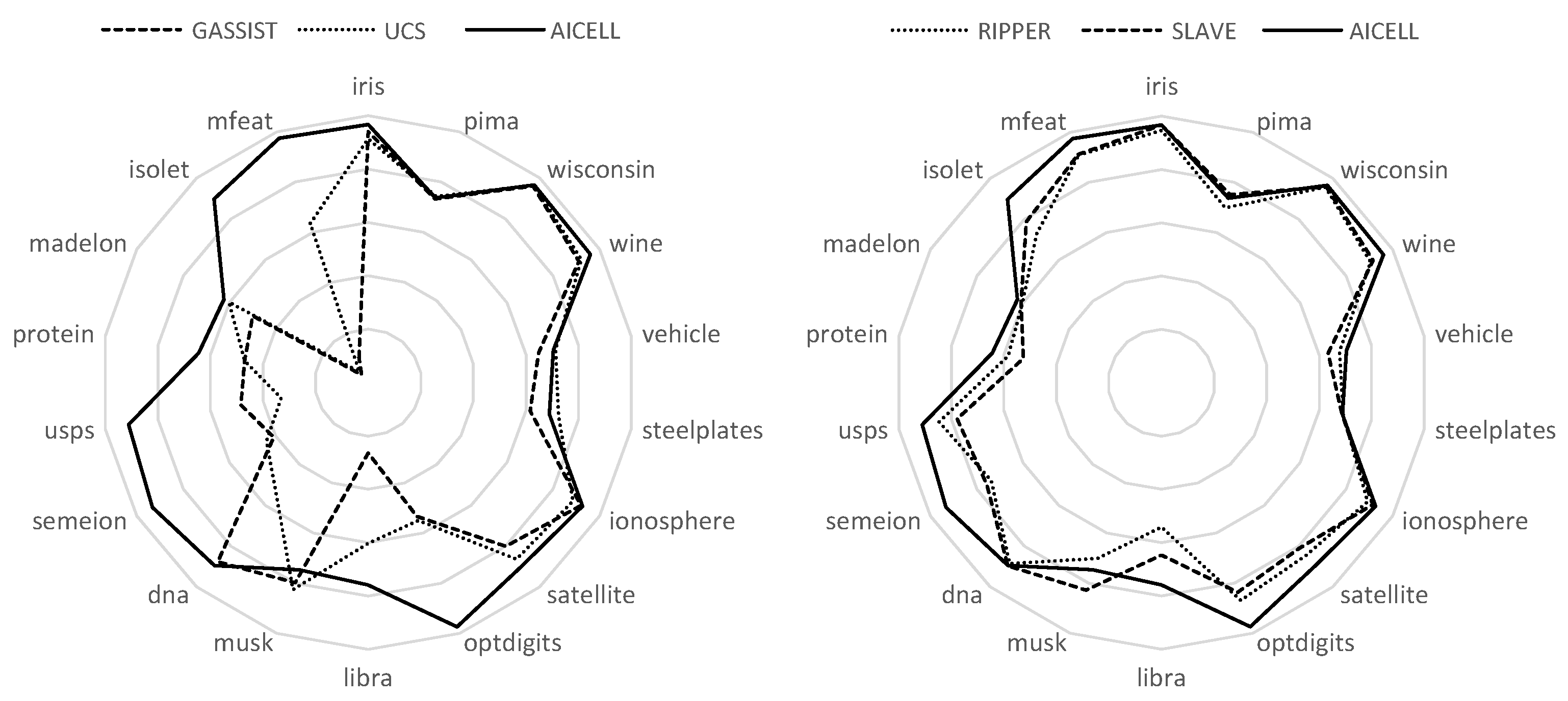
This fact becomes more obvious in the radar plots shown in Figure 3, in which the datasets are listed with the number of attributes increasing clockwise. As obvious, on the right semicircle, where the number of features is relatively small, all algorithms have comparable performances. However, as we move to the left semicircle, the performances of GASSIST and UCS significantly decrease. RIPPER and SLAVE have a more robust performance, but still are significantly behind AICELL in most of the problems.
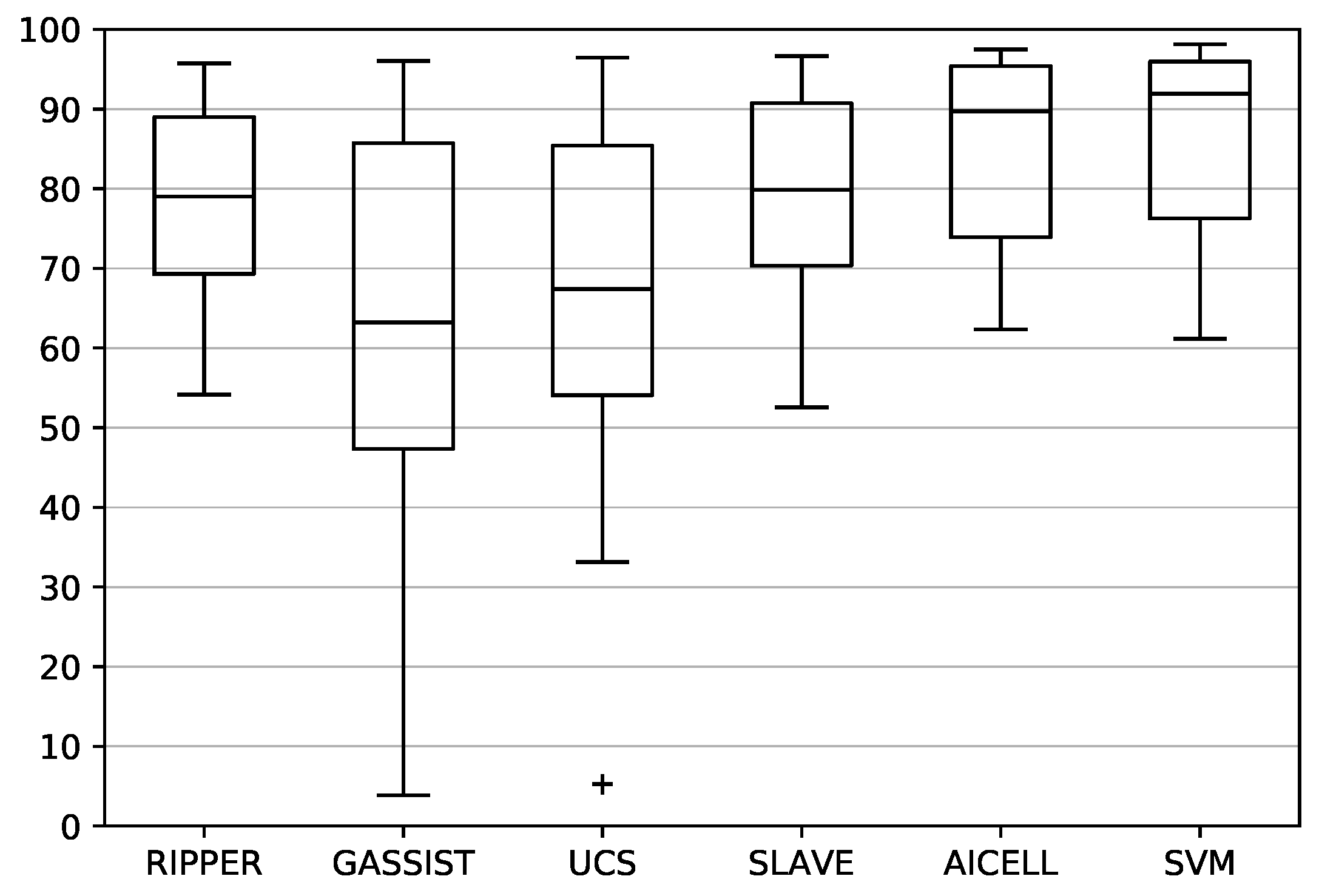
Finally, the distribution of the classifier accuracy on each problem is shown in the box plots of Figure 4. The distribution of AICELL has the best median value. SLAVE and RIPPER follow, with SLAVE being marginally better. Similarly, the worst-case performance of AICELL is better than the worst performances of SLAVE and RIPPER. On the other hand, GASSIST and UCS have significantly inferior overall performances, in terms of both median and worse-case values, with GASSIST being the worst of the two.
10.2. Friedman, Aligned Ranks and Quade Significance Tests.
The values of the significance tests for the Friedman, Aligned ranks and Quade criteria are shown in Table 3. As shown, for the Friedman test, the value of p is in the order of , while for Quade even smaller. For the aligned ranks metric, the value of p is quite larger, however it remains an order of magnitude below the usual threshold of . The results of all tests converge to the conclusion that the differences between the algorithms are statistically significant, and a post-hoc analysis of the results to find the pairwise differences is required.
The results of the post-hoc analysis are shown in Table 4. According to the Friedman criterion, AICELL is better than all algorithms tested. For the comparison to SLAVE, the value of p is marginal, while for the comparisons to the rest of the algorithms the p-value is quite smaller, the differences can safely be regarded as significant. UCS slightly overcomes RIPPER, because of having the best performance of all algorithms in two problems (vehicle and steelplates), while GASSIST has the worst performance among all algorithms.
On the contrary, according to Aligned ranks, SLAVE and RIPPER have somewhat better performances, and their differences from AICELL are not statistically significant. On the contrary UCS and GASSIST have much worse performances. The particular criterion, in contrast to the Friedman test, evaluates the overall distribution of the solutions proposed by each algorithm, and not the per-problem relative performances, and for this reason, the overall conclusions are similar to those acquired by the box plots.
Finally, the Quade test combines the characteristics of the two previous tests, correcting the rank of each algorithm on each problem with the performances of the rest of the algorithms on the same problem. As a result, its outcome lies between the conclusions of the two previous tests. With this criterion too, AICELL seems better than all algorithms, but the difference is significant only for the comparisons to UCS and GASSIST.
10.3. Wilcoxon Rank-Sum and Signed-Rank Significance Tests
The values of the significance tests for the rank-sum and signed-rank criteria are given in Table 5. The rank sum test compares the overall distribution of the algorithms’ performance. According to this criterion, AICELL has the best performance, followed by SLAVE and RIPPER. UCS and GASSIST have significantly worse performances, with similar results. The difference of AICELL to GASSIST and UCS is statistically significant, being an order of magnitute smaller than the required threshold. The difference to RIPPER is not significant (although it comes close to the threshold), while for the comparison to SLAVE the value of p is quite larger, and the performance of the two algorithms can be regarded as comparable. The overall conclusions of this criterion are similar to those of the boxplots.
On the contrary, according to the signed rank test, the ordering of the algorithms is quite different. RIPPER has the worst performance, overtaking AICELL only on the steelplates, and even there with small difference. GASSIST has the second worst performance, being better only in musk, but with bigger difference than RIPPER, while UCS has better performance in 4 problems. However, event with this criterion SLAVE has the second best performance, while AICELL has better performance that all algorithms. Moreover, according to this criterion, the differences are statistically significant for all pairwise comparisons.
10.4. Number of Rules
In Table 6 we list the number of rules of each classifier on each dataset. We omit UCS for which, in contrast to the rest of the classifiers, multiple rules trigger for each pattern, and the class is assigned by voting. However, even if we map its function to that of the other classifiers to render the comparison possible, the number of rules is in general too large, reaching thousands for most of the problems examined.
As shown by the table, GASSIST produces, by far, the smallest number of rules. However, this is the greatest problem of the algorithm, since this number of rules is insufficient for larger problems, and consequently the algorithm performs badly on them. The small number of rules is an inherent characteristic of the algorithm, regardless of the training parameters. Among the remaining algorithms, AICELL produces the smallest number of rules, in terms of both mean and median value. The difference is small in terms and median value, and slightly larger in terms of mean, due to the large number of rules produced by SLAVE and RIPPER in some particular problems, however the overall differences are quite small and cannot be considered important.
10.5. Comparison to SVM
Finally, compared to SVMs, AICELL is surpassed in 13 out of the 18 problems examined. However, the difference in small in gereral, having a mean value of and a median of . This difference is smaller than the difference of AICELL to the second best rule-based algorithm in each problem (mean and median ), and even larger than its difference from the overall second best SLAVE, for which the difference surpasses in terms of both mean and median values.
Moreover, as shown by the significance tests listed in Table 7, the differences are statistically significant only for the signed-rank test, and, even for that metric, the p-value is marginally smaller than the critical threshold. The second largest difference appears in the Friedman test which, like the signed-rank test, evaluates the number of problems in which each classifier has the best performance. On the contrary, for all other metrics, which evaluate the overall solution distribution, the differences are negligible, with the value of p being close to .
However, it must be noted that the performance of SVM listed here is produced by a very extensive cross-validation parameter values, and that for most value pairs, the performance is much worse. On the contrary, AICELL exhibits much more robust behavior in terms of parameter values, while the training duration is also much shorter, by orders of magnitude on some problems. Additionally, the rules produced by AICELL are much simpler.
10.6. Discussion of Results
In this section, the proposed method has been compared with 4 other algorithms that have been widely used in comparisons and are considered state-of-the-art. Among these algorithms, GASSIST and UCS are generally regarded as slightly superior. However, these conclusions have been drawn from experiments on much simpler datasets than the ones examined here, where the number of attributes does not exceed 30, and the number of classes is 2 or 3 (we refer the reader to [36] for detailed comparison). The problems examined here present significantly larger complexity, in terms of both number of attributes and number of classes, the conclusions are considerably different to those presented in the majority of the literature.
In more detail, according to all metrics, GASSIST has the worst performance. Although it achieves satisfying results, while having small number of rules, on the simpler datasets, its performance deteriorates significantly as the number of features and classes increases. These problems have been acknowledged by the creator of the algorithm himself [49]. RIPPER and UCS follow, with UCS having the best performance in some of the problems and very bad in others, especially the more complex ones, while RIPPER, despite not achieving the best performance in any of the problems examined, has satisfactory performance on all of them. SLAVE achieves the best performance, with significant difference, coming first in more problems than the other 3 algorithms, and second in some harder ones. Moreover, the overall distribution of the proposed solutions is much better than that of GASSIST and UCS, and slightly better than that of RIPPER.
According to all the metrics examined, the proposed method achieves the best performance. The difference is statistically significant in all metrics compared to GASSIST, and in most of them compared to UCS. The difference to RIPPER is close to the critical value for most of the tests, while the difference to SLAVE statistically insignificant with most criteria. However, AICELL achieves the best distribution, and has the best performance in larger number of problems than the rest of the algorithms. Moreover, it has consistently good performance in problems with large number of features and classes, achieving large difference from the second best in some of them. Finally, compared to SVM, AICELL is surpassed in most problems, but the difference is marginal and statistically insignificant in most cases, while the training duration and sensitivity to parameter values is much smaller.
11. Conclusions and Future Work
We have proposed in this paper a classification algorithm based on an Artificial Immune Network. The proposed algorithm encodes the patterns to be recognized as antigens, and evolves antibodies representing classification rules of ellipsoidal surface. The antibodies evolve individually, so as to maximize the evaluation metric, resembling in this sense classic Michigan-style classifier rules. Additionally, as happens in most immune networks, antibodies of high similarity or low quality are removed from the network.
However, contrary to most immune algorithms, the aim of the proposed algorithm is not the recognition, but the elimination of the antigens. Antigens that have already been confronted have no further impact on the evolution of the network, which helps minimize the overlap between rules, and guide the new rules towards uncovered areas of the problem space. This brings the algorithm closer to Incremental Rule Learning classifier systems, which have been shown to combine advantages of Pittsburg and Michigan classifiers.
In general, incremental classifiers are not compatible with fuzzy rules, due to the fact that they have to remove patterns that are covered by each new rule, whereas, in fuzzy classifiers, all patterns are covered by all rules. However, the modification employed here enables us to compromise the two approaches, enabling the algorithm to take advantage of the lower number of rules and better generalization ability of fuzzy classifiers. As shown, as the steepness of the membership function increases, the proposed classifier becomes strictly equivalent to an incremental rule classifier.
Regarding more specific algorithm design choices, the recognition rules are based on a quadratic surface, which closely resembles that of an ellipsoid, while being computationally simpler. For the evaluation of the rules a fuzzy generalization of the common m-estimate has been employed. For the removal of unsuitable antibodies from the network, a similarity metric based on the inner product of membership function values has been employed, while antibodies are also removed if the have either lower recognition ability or smaller coverage than the rest of the network population, based on outlier detection criteria. Finally, a rule initialization method was proposed, which further helps the algorithm locate uncovered areas of the problem space.
The proposed method was tested against one representative classifier of each type. On the problems examined, the algorithm had better accuracy than both the Pittsburg and Michigan classifiers. Additionally, it produced much fewer rules than the Michigan classifier, while also performing well in more complex problems, contrary to the Pittsburg classifier, which is limited by its chromosome encoding length. The differences are more obvious in problems with larger number of features and classes, where the proposed method significantly outperformed the competition, maintaining both the robustness and small number of rules exhibited by the incremental rule classifier, and the generalization ability of the fuzzy classifier. Finally, compared to Support Vector Machines, the algorithm was surpassed in the majority of the problems, however the differences are marginal and statistically insignificant, while the proposed method is much more robust to the change of training parameters, and generates much simpler and more interpretable rules.
Regarding possible extensions of the present algorithm, the main area to experiment with is the employment of different geometries of recognition rules and different shapes of membership functions. Since different shapes of surfaces could be more appropriate for covering different areas of the problem space, it would be beneficial to combine multiple forms of rules within the same classifier. Additionally the evaluation metric could be extended so that, during the training of each rule, it also takes into account the existing rules, further assisting cooperation.
Author Contributions
A.L., G.S. and A.S conceived the algorithm. A.L. developed and implemented the model. A.L. and G.S. performed experiments. A.L., G.S. and A.S. analyzed the data. A.L., G.S. and A.S wrote the paper.
Conflicts of Interest
The authors declare no conflict of interest.
References
- Burnet, F.M. The Clonal Selection Theory of Acquired Immunity; Vanderbilt University Press: Nashville, TN, USA, 1959; p. 232. [Google Scholar]
- Jerne, N. Towards a network theory of the immune system. Ann. Immunol. 1974, 125, 373–389. [Google Scholar]
- De Castro, L.N.; Timmis, J. Artificial Immune Systems: A New Computational Intelligence Approach; Springer: London, UK, 2002. [Google Scholar]
- De Castro, L.N.; Von Zuben, F.J. Learning and Optimization Using the Clonal Selection Principle. IEEE Trans. Evol. Comput. 2002, 6, 239–251. [Google Scholar] [CrossRef]
- De Castro, L.N.; Zuben, F.J.V. aiNet: An Artificial Immune Network for Data Analysis. In Data Mining: A Heuristic Approach; Abbass, H.A., Sarker, R.A., Newton, C.S., Eds.; Idea Group Publishing: Hershey, PA, USA, 2001; pp. 231–259. [Google Scholar]
- Karakasis, V.K.; Stafylopatis, A. Efficient Evolution of Accurate Classification Rules Using a Combination of Gene Expression Programming and Clonal Selection. IEEE Trans. Evol. Comput. 2008, 12, 662–678. [Google Scholar] [CrossRef]
- Lanaridis, A.; Stafylopatis, A. An Artificial Immune Network for Multiobjective Optimization Problems. Eng. Optim. 2013, 46, 1008–1031. [Google Scholar] [CrossRef]
- Magna, G.; Casti, P.; Jayaraman, S.V.; Salmeri, M.; Mencattini, A.; Martinelli, E.; Natale, C.D. Identification of mammography anomalies for breast cancer detection by an ensemble of classification models based on artificial immune system. Knowl. Based Syst. 2016, 101, 60–70. [Google Scholar] [CrossRef]
- Martinelli, E.; Magna, G.; Vito, S.D.; Fuccio, R.D.; Francia, G.D.; Vergara, A.; Natale, C.D. An adaptive classification model based on the Artificial Immune System for chemical sensor drift mitigation. Sens. Actuators B Chem. 2013, 177, 1017–1026. [Google Scholar] [CrossRef]
- Lanaridis, A.; Stafylopatis, A. An Artificial Immune Classifier Using Pseudo-Ellipsoid Rules. In Proceedings of the 26th International Symposium on Computer and Information Sciences, London, UK, 26–28 September 2011; pp. 395–401. [Google Scholar]
- Hyafil, L.; Rivest, R.L. Constructing optimal binary decision trees is NP-complete. Inf. Proc. Lett. 1976, 5, 15–17. [Google Scholar] [CrossRef]
- Holland, J.H. Adaptation in Natural and Artificial Systems: An Introductory Analysis with Applications to Biology, Control and Artificial Intelligence; University of Michigan Press: Ann Arbor, MI, USA, 1975. [Google Scholar]
- Sigaud, O.; Wilson, S.W. Learning classifier systems: A survey. Soft Comput. 2007, 11, 1065–1078. [Google Scholar] [CrossRef]
- Smith, S.F. A Learning System Based on Genetic Adaptive Algorithms. Ph.D. Thesis, University of Pittsburg, Pittsburgh, PA, USA, 1980. [Google Scholar]
- Holland, J.; Reitman, J. Cognitive Systems Based on Adaptive Algorithms; Department of Computer and Communication Science, University of Michigan: Ann Arbor, MI, USA, 1977. [Google Scholar]
- Venturini, G. SIA: A Supervised Inductive Algorithm with Genetic Search for Learning Attributes Based Concepts. In Machine Learning: ECML ’93, Lecture Notes on Computer Science; Springer: London, UK, 1993; pp. 280–296. [Google Scholar]
- Garrett, S.M. How Do We Evaluate Artificial Immune Systems? Evol. Comput. 2005, 13, 145–177. [Google Scholar] [CrossRef] [PubMed]
- Hart, E.; Timmis, J. Application Areas of AIS: The Past, the Present and the Future. Appl. Soft Comput. 2008, 8, 191–201. [Google Scholar] [CrossRef]
- De Castro, L.N.; Timmis, J. Artificial Immune Systems: A New Computational Intelligence Paradigm; Springer-Verlag New York, Inc.: Secaucus, NJ, USA, 2002. [Google Scholar]
- Abe, S. Dynamic cluster generation for a fuzzy classifier with ellipsoidal regions. IEEE Trans. Syst. Man Cybern. Part B 1998, 28, 869–876. [Google Scholar] [CrossRef] [PubMed]
- Yao, L.; Lin, C.C. A fuzzy classifier with evolutionary design of ellipsoidal decision regions. Proc. World Acad. Sci. Eng. Tech. 2005, 1, 38–44. [Google Scholar]
- Abe, S.; Thawonmas, R. A fuzzy classifier with ellipsoidal regions. Fuzzy Syst. IEEE Trans. 1997, 5, 358–368. [Google Scholar] [CrossRef]
- Yao, L.; Weng, K.S.; Huang, C.D. Evolutionary design of fuzzy classifier with ellipsoidal decision regions. In Proceedings of the 2005 IEEE International Conference on Systems, Man and Cybernetics, Waikoloa, HI, USA, 12 October 2005; Volume 1, pp. 785–790. [Google Scholar]
- Michalewicz, Z. Genetic Algorithms + Data Structures = Evolution Programs; Springer: New York, NY, USA, 1996. [Google Scholar]
- Goldberg, D.E. Genetic Algorithms in Search, Optimization, and Machine Learning; Addison-Wesley: Boston, MA, USA, 1989. [Google Scholar]
- Nada Lavrac, P.A.F.; Zupan, B. Rule Evaluation Metrics: A unifying view. In Proceedings of the 9th International Workshop on Inductive Logic Programming, Bled, Slovenia, 24–27 June 1999; pp. 173–185. [Google Scholar]
- Furnkranz, J.; Flach, P.A. An Analysis of Rule Evaluation Metrics. In Proceedings of the 20th International Conference on Machine Learning (ICML-2003), Washington, DC, USA, 21–24 August 2003; pp. 202–209. [Google Scholar]
- Furnkranz, J.; Flach, P. An Analysis of Rule Learning Heuristics. 2007. Available online: http://citeseer.ist.psu.edu/viewdoc/summary?doi=10.1.1.60.3804 (accessed on 15 June 2017).
- Tukey, J. Comparing Individual Means in the Analysis of Variance. Biometrics 1949, 2, 99–114. [Google Scholar] [CrossRef]
- Chang, C.C.; Lin, C.J. LIBSVM: A Library for Support Vector Machines. ACM Trans. Intell. Syst. Technol. 2011, 2. [Google Scholar] [CrossRef]
- Bache, K.; Lichman, M. UCI Machine Learning Repository. 2013. Available online: http://archive.ics.uci.edu/ml (accessed on 15 February 2017).
- Cohen, W. Fast Effective Rule Induction. In Proceedings of the Twelfth International Conference on Machine Learning, Tahoe City, CA, USA, 9–12 July 1995; pp. 1–10. [Google Scholar]
- Bacardit, J.; Garrell, J. Evolving multiple discretizations with adaptive intervals for a pittsburgh rule-based learning classifier system. In Proceedings of the GECCO 2003 Genetic and Evolutionary Computation Conference, Chicago, IL, USA, 12–16 July 2003; pp. 1818–1831. [Google Scholar]
- Gonzalez, A.; Perez, R. Selection of relevant features in a fuzzy genetic learning algorithm. IEEE Trans. Syst. Man Cybern. Part B 2001, 31, 417–425. [Google Scholar] [CrossRef] [PubMed]
- Bernado-Mansilla, E.; Garrell, J. Accuracy-Based Learning Classifier Systems: Models and Analysis and Applications to Classification Tasks. Evol. Comput. 2003, 11, 209–238. [Google Scholar] [CrossRef] [PubMed]
- Fernandez, A.; Garcia, S.; Luengo, J.; Bernando-Mansilla, E.; Herrera, F. Genetics-Based Machine Learning for Rule Induction: State of the Art, Taxonomy, and Comparative Study. Evol. Comput. IEEE Trans. 2010, 14, 913–941. [Google Scholar] [CrossRef]
- Friedman, M. A Comparison of Alternative Tests of Significance for the Problem of m Rankings. Ann. Math. Stat. 1940, 11, 86–92. [Google Scholar] [CrossRef]
- Hodges, J.L.; Lehmann, E.L. Rank methods for combination of independent experiments in analysis of variance. Ann. Math. Stat. 1960, 6, 403–418. [Google Scholar]
- Quade, D. Using Weighted Rankings in the Analysis of Complete Blocks with Additive Block Effects. J. Am. Stat. Assoc. 1979, 74, 680–683. [Google Scholar] [CrossRef]
- Wilcoxon, F. Individual comparisons by ranking methods. Biom. Bull. 1945, 1, 80–83. [Google Scholar] [CrossRef]
- Derrac, J.; Garcia, S.; Molina, D.; Herrera, F. A practical tutorial on the use of nonparametric statistical tests as a methodology for comparing evolutionary and swarm intelligence algorithms. Swarm Evol. Comput. 2011, 1, 3–18. [Google Scholar] [CrossRef]
- Demvsar, J. Statistical Comparisons of Classifiers over Multiple Data Sets. J. Mach. Learn. Res. 2006, 7, 1–30. [Google Scholar]
- Garcia, S.; Herrera, F.; Shawe-Taylor, J. An extension on statistical comparisons of classifiers over multiple data sets for all pairwise comparisons. J. Mach. Learn. Res. 2008, 9, 2677–2694. [Google Scholar]
- Alcala-Fdez, J.; Sanchez, L.; Garcia, S.; del Jesus, M.; Ventura, S.; Garrell, J.; Otero, J.; Romero, C.; Bacardit, J.; Rivas, V.; et al. KEEL: A software tool to assess evolutionary algorithms for data mining problems. Soft Comput. 2009, 13, 307–318. [Google Scholar] [CrossRef]
- Alcala-Fdez, J.; Fernandez, A.; Luengo, J.; Derrac, J.; Garcia, S. KEEL Data-Mining Software Tool: Data Set Repository, Integration of Algorithms and Experimental Analysis Framework. Mult. Valued Log. Soft Comput. 2011, 17, 255–287. [Google Scholar]
- Joachims, T. Making large-Scale SVM Learning Practical. In Technical Report, SFB 475: Komplexitätsreduktion in Multivariaten Datenstrukturen; Universität Dortmund: Dortmund, Germany, 1998. [Google Scholar]
- Knerr, S.; Personnaz, L.; Dreyfus, G. Single-layer learning revisited: A stepwise procedure for building and training a neural network. In Neurocomputing; Springer: Berlin, Germany, 1990; pp. 41–50. [Google Scholar]
- Galar, M.; Fernandez, A.; Barrenechea, E.; Bustince, H.; Herrera, F. An overview of ensemble methods for binary classifiers in multi-class problems: Experimental study on one-vs-one and one-vs-all schemes. Pattern Recognit. 2011, 44, 1761–1776. [Google Scholar] [CrossRef]
- Bacardit, J. Pittsburgh Genetics-Based Machine Learning in the Data Mining Era: Representations, generalization, and run-time. Ph.D. Thesis, Ramon Llull University, Barcelona, Spain, 2004. [Google Scholar]
Figure 1.
Comparison between the random and health-proportional initialization. The figure displays the decrease of average antigen health with the number of training generations t. As evident from the figure, the proposed method results in faster convergence and smaller deviation between runs.
Figure 1.
Comparison between the random and health-proportional initialization. The figure displays the decrease of average antigen health with the number of training generations t. As evident from the figure, the proposed method results in faster convergence and smaller deviation between runs.
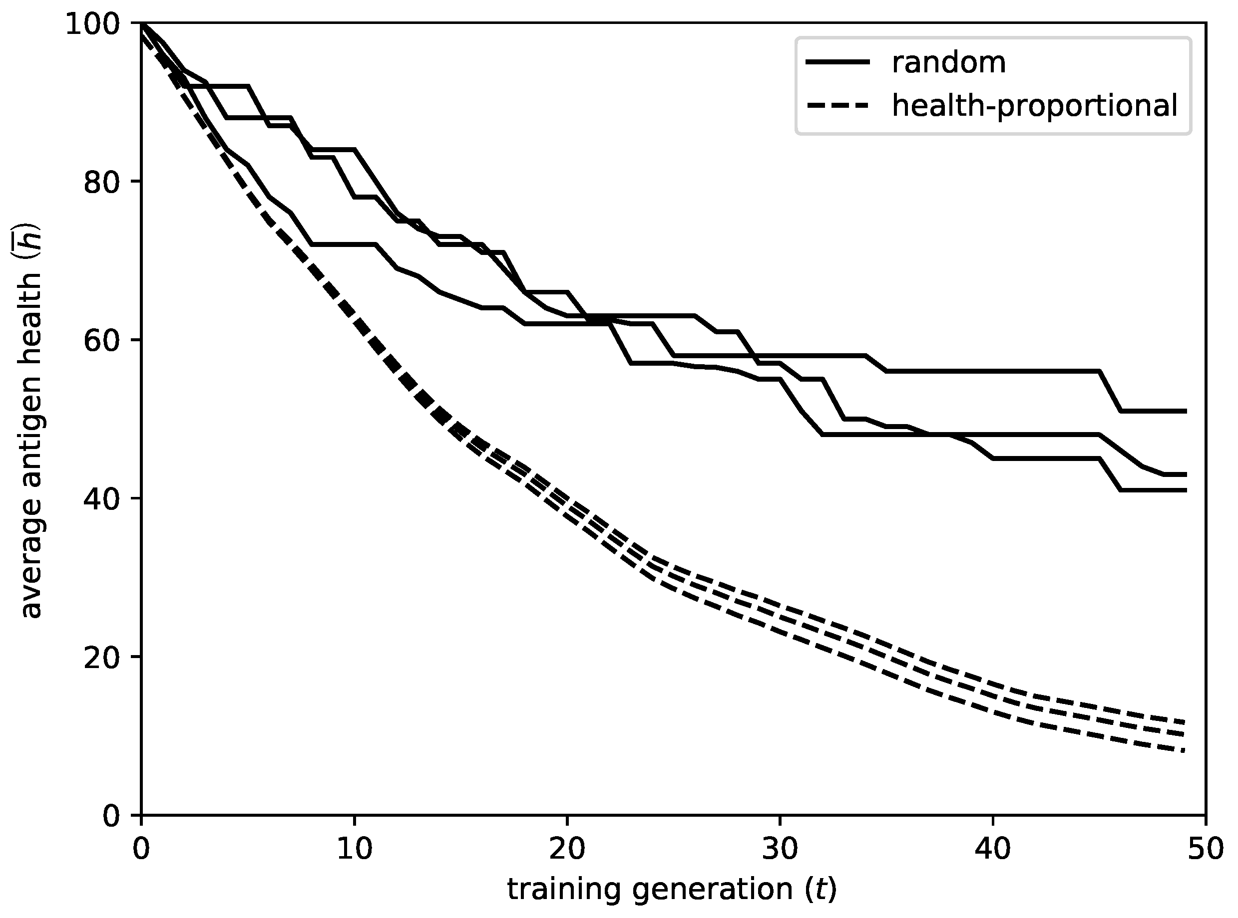
Figure 2.
Removing rules of lower quality. The two rules in the center of (a) are inferior to the rest, one of them because it covers many patterns of the wrong class and the other because of its small coverage. Although the value of their evaluation metric, shown in (b), is indeed lower, they cannot be easily detected based on that value. However, by breaking the metric down to its coverage and precision components, the differences become much clearer, and the two rules can be rejected as outliers.

Figure 3.
Performance of all classifiers on all problems, ordered clockwise in increasing number of features. As obvious, the performances of GASSIST and UCS significantly decrease as the number of features increases. For RIPPER and SLAVE the differences are significantly smaller, however their overall performance is inferior to that of AICELL.Radar plots

Figure 4.
Boxplot of the precision of the algorithms tested on the problems mentioned. GASSIST and UCS fall behind in terms of both mean and median value. RIPPER has comparable distribution to SLAVE, despite not having the best performance in any problem. AICELL has the best overall performance, coming very close to SVM.

Table 1.
Datasets used for the evaluation of the algorithms. The datasets are ordered in increasing number of attributes, and for each one the number of classes and instances are listed. On problems where a test set is not provided, 5-fold cross-validation was used.
Table 1.
Datasets used for the evaluation of the algorithms. The datasets are ordered in increasing number of attributes, and for each one the number of classes and instances are listed. On problems where a test set is not provided, 5-fold cross-validation was used.
| Dataset | Attributes | Classes | Training | Test |
|---|---|---|---|---|
| iris | 4 | 3 | 150 | |
| pima | 8 | 2 | 768 | |
| wisconsin | 9 | 2 | 683 | |
| wine | 13 | 3 | 178 | |
| vehicle | 18 | 4 | 846 | |
| steelplates | 27 | 7 | 1941 | |
| ionosphere | 34 | 2 | 351 | |
| satellite | 36 | 6 | 2000 | 4435 |
| optdigits | 64 | 10 | 3823 | 1797 |
| libra | 90 | 15 | 360 | |
| musk | 166 | 2 | 476 | |
| dna | 180 | 3 | 1400 | 1186 |
| semeion | 256 | 10 | 1593 | |
| usps | 256 | 10 | 7291 | 2007 |
| protein | 357 | 3 | 17,766 | 6621 |
| madelon | 500 | 2 | 2000 | 600 |
| isolet | 617 | 26 | 6238 | 1559 |
| mfeat | 649 | 10 | 2000 |
Table 2.
Precision of the algorithms on the test dataset.
| Dataset | RIPPER | GASSIST | UCS | SLAVE | AICELL | SVM |
|---|---|---|---|---|---|---|
| iris | ||||||
| pima | ||||||
| wisconsin | ||||||
| wine | ||||||
| vehicle | ||||||
| steelplates | ||||||
| ionosphere | ||||||
| satellite | ||||||
| optdigits | ||||||
| libra | ||||||
| musk | ||||||
| dna | ||||||
| semeion | ||||||
| usps | ||||||
| protein | ||||||
| madelon | ||||||
| isolet | ||||||
| mfeat |
Table 3.
Results of the Friedman, Aligned ranks and Quade Significance tests. For each test we list the rank of each algorithm, the corresponding z-value, the distributions, and the p-value.
Table 3.
Results of the Friedman, Aligned ranks and Quade Significance tests. For each test we list the rank of each algorithm, the corresponding z-value, the distributions, and the p-value.
| Algorithm | Friedman | Aligned Ranks | Quade |
|---|---|---|---|
| RIPPER | |||
| GASSIST | |||
| UCS | |||
| SLAVE | |||
| AICELL | |||
| value | |||
| distribution | |||
| p-value | 7.0454 × | 4.98852 × | 1.4048 × |
Table 4.
Post-hoc analysis for the Friedman, Aligned ranks and Quade significance tests.
| Criterion | Algorithm | Rank | z-Value | p-Value |
|---|---|---|---|---|
| Friedman | RIPPER | 3 | 5.0421 × | |
| GASSIST | 4 | 3.1817 × | ||
| UCS | 2 | 7.4327 × | ||
| SLAVE | 1 | 4.5201 × | ||
| Aligned ranks | RIPPER | 2 | 7.5088 × | |
| GASSIST | 4 | 1.6851 × | ||
| UCS | 3 | 2.1075 × | ||
| SLAVE | 1 | 2.7251 × | ||
| Quade | RIPPER | 2 | 5.3208 × | |
| GASSIST | 4 | 2.9040 × | ||
| UCS | 3 | 1.0576 × | ||
| SLAVE | 1 | 2.4734 × |
Table 5.
Wilcoxon rank-sum and signed-rank tests.
| Criterion | Algorithm | z-Value | p-Value | h | ||
|---|---|---|---|---|---|---|
| rank sum | RIPPER | 0 | ||||
| GASSIST | 421 | 245 | 1 | |||
| UCS | 424 | 242 | 1 | |||
| SLAVE | 0 | |||||
| signed rank | RIPPER | 170 | 1 | 2.332 × | 1 | |
| GASSIST | 164 | 7 | 6.292 × | 1 | ||
| UCS | 150 | 21 | 1 | |||
| SLAVE | 1 |
Table 6.
Number of rules of the classifiers on each of the problems examined.
| Dataset | RIPPER | GASSIST | SLAVE | AICELL |
|---|---|---|---|---|
| iris | 6.2 | 4.2 | 3 | 6.4 |
| pima | 25.6 | 6.6 | 15.8 | 9.4 |
| wisconsin | 8.2 | 4.4 | 4.6 | 4.2 |
| wine | 6 | 4.2 | 3.6 | 6.2 |
| vehicle | 39.4 | 6.4 | 29.8 | 47.2 |
| steelplates | 80.4 | 6.2 | 50.6 | 58.2 |
| ionosphere | 12.2 | 4.6 | 3.2 | 11.2 |
| satellite | 65 | 9 | 46 | 51 |
| optdigits | 86 | 12 | 62 | 87 |
| libra | 51 | 10.4 | 46.4 | 60.8 |
| musk | 15.4 | 4.8 | 16.8 | 20.5 |
| dna | 31 | 5 | 32 | 34 |
| semeion | 80.2 | 11.4 | 71.8 | 46.4 |
| usps | 129 | 16 | 96 | 66 |
| protein | 172 | 2 | 1390 | 14 |
| madelon | 37 | 2 | 47 | 74 |
| isolet | 211 | 2 | 138 | 45 |
| mfeat | 37.6 | 2 | 41.4 | 21.8 |
| mean | 56.6 | 8.7 | 116.9 | 35.5 |
| median | 37.3 | 4.9 | 43.7 | 34 |
Table 7.
Comparison to SVM. Although the performance of SVM is better than that of AICELL with all metrics, the difference is statistically significant only for the Wilcoxon signed-rank test, and even for that, with a marginal p-value, while for the rest of the metrics the p-value is an order of magnitude above the critical threshold.
| Criterion | z-Value | p-Value | ||
|---|---|---|---|---|
| Friedman | ||||
| Aligned ranks | ||||
| Quade | ||||
| Rank sum | 310 | 356 | ||
| Signed rank | 39 | 132 |
© 2017 by the authors. Licensee MDPI, Basel, Switzerland. This article is an open access article distributed under the terms and conditions of the Creative Commons Attribution (CC BY) license (http://creativecommons.org/licenses/by/4.0/).
Share and Cite
MDPI and ACS Style
Lanaridis, A.; Siolas, G.; Stafylopatis, A. Artificial Immune Classifier Based on ELLipsoidal Regions (AICELL) †. Computation 2017, 5, 31. https://doi.org/10.3390/computation5020031
AMA Style
Lanaridis A, Siolas G, Stafylopatis A. Artificial Immune Classifier Based on ELLipsoidal Regions (AICELL) †. Computation. 2017; 5(2):31. https://doi.org/10.3390/computation5020031
Chicago/Turabian StyleLanaridis, Aris, Giorgos Siolas, and Andreas Stafylopatis. 2017. "Artificial Immune Classifier Based on ELLipsoidal Regions (AICELL) †" Computation 5, no. 2: 31. https://doi.org/10.3390/computation5020031
Note that from the first issue of 2016, this journal uses article numbers instead of page numbers. See further details here.