Optimization of Airfoils Using the Adjoint Approach and the Influence of Adjoint Turbulent Viscosity


1
ForWind, University of Oldenburg, Ammerländer Heerstr. 114-118, 26129 Oldenburg, Germany
2
Fraunhofer Institute for Wind Energy Systems, Küpkersweg 70, 26129 Oldenburg, Germany
*
Author to whom correspondence should be addressed.
Computation 2018, 6(1), 5; https://doi.org/10.3390/computation6010005
Submission received: 29 September 2017
/
Revised: 12 January 2018
/
Accepted: 17 January 2018
/
Published: 20 January 2018
(This article belongs to the Special Issue Computational Methods in Wind Engineering)
Abstract
:The adjoint approach in gradient-based optimization combined with computational fluid dynamics is commonly applied in various engineering fields. In this work, the gradients are used for the design of a two-dimensional airfoil shape, where the aim is a change in lift and drag coefficient, respectively, to a given target value. The optimizations use the unconstrained quasi-Newton method with an approximation of the Hessian. The flow field is computed with a finite-volume solver where the continuous adjoint approach is implemented. A common assumption in this approach is the use of the same turbulent viscosity in the adjoint diffusion term as for the primal flow field. The effect of this so-called “frozen turbulence” assumption is compared to the results using adjoints to the Spalart–Allmaras turbulence model. The comparison is done at a Reynolds number of for two different airfoils at different angles of attack.
1. Introduction
The design of aerodynamic shapes is increasingly based on Computational Fluid Dynamics (CFD). Since CFD is computationally more expensive than the coupling of potential flow theory with boundary layer corrections, a computationally inexpensive optimization technique is preferable. Stochastic search optimization methods require a large number of function evaluations [1], but gradient-based optimizations can be used in order to have fewer function calls. Gradients can be computed via finite differencing, however, the computational cost scales linearly with the number of design parameters [2]. In the adjoint approach, the influence of the primal flow field is decoupled from the gradients depending on the design parameters. This results in another set of Partial Differential Equations (PDEs), the adjoint equations, in which each adjoint variable refers to a variable of the flow field. Solving the adjoint equations has a comparable cost to solving the primal state equations [3] and the gradients can be computed from primal and adjoint fields with minor additional calculations compared to the CFD iterations. Practically, the gradient evaluation cost does not scale with the number of design parameters, in contrast to traditional finite differencing. Thus, the adjoint approach is often combined when using gradient-based optimization with many design parameters and CFD.
Two types of adjoint methods are known from the literature: the discrete method and the continuous method [4,5,6]. In the discrete approach, the adjoint equations are generated from the discretized flow equations, often via an automatic differentiation tool. This method is strongly connected to the selected flow solver and the discretization schemes of the primal state equations. If no approximations are used, the discrete approach leads to the exact gradients of the original discretized flow equations, but tend to have higher memory requirements [5].
In the continuous approach, the adjoint equations are derived analytically from the flow equations and are subsequently discretized. The discretization schemes can be different than the schemes of the primal flow equations and the continuous adjoints may need less memory as well as less computational effort [4,7]. The “physical significance of the adjoint variables is much clearer” [4] than in the discrete approach. It can be seen from the analytical adjoint equations that the adjoint field develops backwards in time and upstream to the primal flow. A known disadvantage of the continuous adjoint approach is that it can produce inaccurate gradients in turbulent flows [8], because the adjoints to the turbulence parameters are often neglected. This is the so-called “frozen turbulence” assumption [9]: The same turbulent viscosity from the primal Navier–Stokes equations is used in the adjoint equations.
In the first publications, discrete adjoints with “differentiated” turbulence models were implemented without an investigation of the effect on the optimization compared to frozen turbulence [10,11]. Lyu et al. [12] used discrete adjoints and the Spalart–Allmaras turbulence model for compressible flows. For the flow over a bump as simple verification case, they found clear differences between the gradients by frozen and adjoint turbulence. The main focus of their work was on the optimization of the ONERA M6 wing and the results of the optimizations were slightly better with adjoint turbulence, but there were also higher computational costs. Osusky et al. [13] used discrete adjoints for drag reduction of wings in compressible flows. They compared the results by optimizations based on Euler and Reynolds-averaged Navier–Stokes (RANS) equations using the Spalart–Allmaras model and obtained inferior designs by the inviscid flow analysis. Besides other approximations, Dwight and Brezillon [14] investigated the effect of frozen turbulence, there called the “constant eddy-viscosity assumption”. They used discrete adjoints in compressible flows and optimized airfoils at small angles of attack without any separation. In an optimization of a transonic airfoil, the frozen turbulence led to poorer optimization behavior compared to the exact adjoint gradients. In an optimization of a subsonic high-lift configuration, the gradients via frozen turbulence were as good as the exact gradients, but it is not clear if these results also hold for continuous adjoints in incompressible flows.
Zymaris et al. [15] derived a continuous adjoint approach to the Spalart–Allmaras turbulence model [16] in incompressible flows. They focused on the verification of the adjoint gradients for duct flows and investigated the effect of different terms in the adjoint turbulence model as well as in its boundary conditions. The resulting effect of frozen turbulence in external flows was not described. Bueno-Orovio et al. [17] derived a continuous adjoint approach to the Spalart–Allmaras model in compressible flows. For a transonic airfoil as well as a transonic wing at a small angle of attack, they showed that the frozen turbulence assumption leads to poorer optimization results compared to the shapes resulting from the inclusion of the adjoint turbulent viscosity. Papoutsis-Kiachagias and Giannakoglou [5] provided a good survey of the adjoints for turbulent flows, where they derived and extended various theoretical aspects. They also verified gradients at two-dimensional airfoils and computed sensitivities for different aerodynamic shapes. Several industrial examples are shown, but an airfoil optimization using the presented approaches is not discussed. Kavvadias et al. [18] derived the continuous adjoints approach to the k-- turbulence model and verified the resulting gradients. Optimization results of ducts using frozen and adjoint turbulence are shown. Also, an optimization of an airfoil with thickness constraint is presented, where the gradients of both approaches are compared as well. However, a detailed comparison of the optimization results using frozen and adjoint turbulence for airfoil shapes is missing.
Since the effect of adjoint turbulence in the continuous approach on the resulting shapes in incompressible, subsonic flows around airfoils have been rarely investigated, it is the aim of our work to compare these results to frozen turbulence in airfoil optimization. Besides, a complete procedure for shape optimization is presented, which may inspire interested readers to develop their own frameworks. The continuous adjoints are used and the adjoints to the turbulence model are implemented following the derivation by Zymaris et al. [15]. The incompressible, steady-state Reynolds-averaged Navier–Stokes equations (RANS) are closed by the Spalart–Allmaras turbulence model [16] without transition. The flow is computed with the open-source code OpenFOAM-2.3.0 [19] based on the Finite Volume Method (FVM). The code is written in C++ and strongly uses the capabilities of object-oriented programming. Although Towara and Naumann [20] use discrete adjoints with OpenFOAM, more often the continuous approach is followed when using this flow solver [21,22]. As this code is very suitable for the implementation of analytical equations, as well as the expected lower memory costs, continuous adjoints are used in our work. The basic equations of this approach have already been implemented by Othmer et al. [23], but their implementation has been made for ducted flows. There, the flow is optimized via a change of the cell porosity, modeling “walls” by obstacles with high porosity blocking. In our work, the shape of the airfoil is changed by the motion of the mesh and the solver is extended to external aerodynamics. The comparison is done for two airfoils and at different angles of attack in order to change the flow complexity.
As an outline for this work, firstly the implementation of a precise and stable mesh motion, which is essential for the later processes, is described in Section 2. Then, a short description of the general adjoint approach follows in Section 3 with the details and simplifications made in the presented implementation. The gradients by the adjoint method are verified and the projection of the gradients to a spline parametrization is described. Finally in Section 4, the effects of frozen and adjoint turbulence on shape optimization of airfoils in incompressible flows are compared.
2. Mesh Motion
During the optimization process, the flow around the changed shape has to be re-computed, which means that the mesh has either to be “re-meshed” completely or the mesh points have to be moved from their previous or initial position. The former approach is more suitable for large geometry changes, but requires more time. The latter method is more suitable for small changes in the shape and requires less time. In any case, it is essential for the optimization that the generated mesh delivers smooth results of the objective function in order to have low noise in the gradients. The flow simulations have to be independent from the mesh deformation.
Since the expected changes in the airfoil shapes are small, the mesh is moved during the optimization in this work. The mesh motion techniques in OpenFOAM are made for general purposes and are not necessarily suitable for airfoil design. Internal tests led to deformed or even overlapping cells, which are obstructive for the computation of the flow around airfoils, in particular in the boundary layer. In order to accurately resolve the boundary layer flow, the meshes at high Reynolds numbers (Re) have a small off-wall distance. Any inaccuracies in mesh deformation such as overlapping cells, increased skewness, or higher non-orthogonality can disrupt the whole optimization process. This is why a robust mesh motion technique is implemented based on the principle from Jameson and Reuther [24]. In a hexahedral mesh, the points in the near and far field are moved according to the movement of the surface points . For this purpose, each surface point is considered as the starting point of a spline reaching from the airfoil to the end of the domain. This is shown in an example in Figure 1 for a single spline.
In order to keep the far-field borders of the domain constant, the motion is linearly interpolated with a factor ( at the airfoil and at the far field):
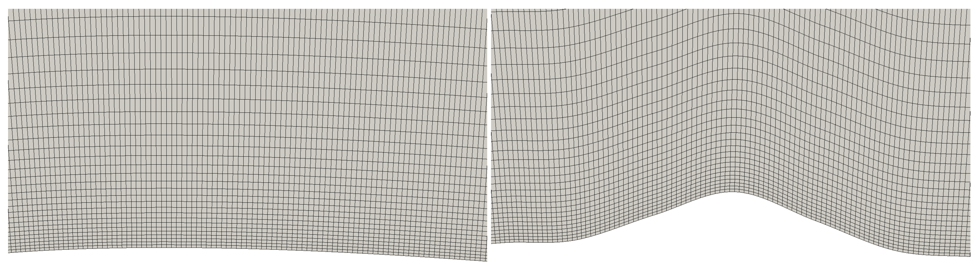
where represents the point positions of the numerical grid and the index S stands for the airfoil surface. In order to show the capabilities of this mesh motion, an example is shown in Figure 2 as a close-up view of the suction side of an airfoil.
The initial mesh is deformed via different spline coordinates of the airfoil and the produced bump on the airfoil is smoothly transferred into the internal mesh with a linear relaxation as in Equation (1). The deformations of the following sections are much smaller and this example is only used in order to show the capabilities of this technique.
As implemented here, the motion technique works only for hexahedral meshes, but for small and smooth shape changes it ensures the same quality of the boundary layer close to the geometry, which is an essential requirement for a successful optimization.
3. The Adjoint Approach
3.1. The General Principle
The derivation of the adjoint approach can be found in the literature [3,4,9,10,15,25,26] and for the sake of brevity only the basic principles are described here according to the notation of Soto and Löhner [27]. Let I be the objective function, which shall be optimized with respect to the design parameters , and be the steady-state incompressible Navier–Stokes equations. Then, the optimization problem can be written as:
where are flow variables in the flow domain . Objective function and equality constraints can be combined via a Lagrange function L:
where are the Lagrangian multipliers or as they are often called, the adjoint variables. A variation of the Lagrangian leads to:
where denote the adjoints to velocity and pressure.
The adjoint variables can now be defined in such a way that the last two brackets become zero, which leads to a new set of PDEs for the adjoint variables, making independent of any variation of the flow field. Equation (4) then simplifies to the following gradient expression:
Since the flow field does not have to be computed for each design variable again as with finite differences, this basically means that the gradient computation becomes independent from the amount of design parameters. As a matter of fact, some extra computations have to be done, which scale with the number of design parameters, but these are insignificant compared with the effort of the remaining CFD iterations. Finally, the geometry can be parametrized by every surface grid point without an increase in the computational costs, which is the strength of the adjoint approach.
3.2. Adjoint Equations and Gradient Calculation
The general adjoint equations are derived via integration by parts from the Navier–Stokes equations. Further details can be found in common literature [15,23,25,27], where the following form is often found for steady-state and incompressible flows:
with the kinematic viscosity . The first term on the left-hand side of Equation (6), the so-called “adjoint transpose convection”, can lead to diverging simulations. Following the suggestions from Önder [21] and Choi et al. [28], the integration by parts is not necessary in the derivation of the adjoint transpose convection. This leads to the following more stable adjoint momentum equation, which is used in this work:
Soto and Löhner [27] derived the gradients for the optimization of total forces (pressure-based and viscous) leading to the following expression:
where S is the domain boundary at the airfoil. Due to a zero Neumann boundary condition of the pressure at the geometry, the first integral vanishes and omitting the second order term leads to an expression similar to the one of other authors [9,15,25,29]. Castro et al. [25] showed that the so-called “geometric term” in Equation (9) vanishes in the case of force optimization (for fully converged solutions of the incompressible or compressible Navier–Stokes equations). This was also shown by others [29,30] in different ways and thus, Equation (9) is further simplified to the final expression used in this work:
where from the authors’ experience the last term is the most dominant one, independent of the Reynolds number.
Since there is no effect of the objective function in Equation (10), the boundary conditions (BCs) have to include a connection to the objectives of the optimization. Zymaris et al. [15] derive the mathematically correct boundary conditions for the far field and walls. From the authors’ experience at small, laminar Reynolds numbers, the correct boundary conditions at the far field do not affect the gradient at the airfoil (unless the domain is too small), but can easily lead to unstable convergence behavior. This is why here, standard Dirichlet and Neumann boundary conditions are used at the far field, where the adjoint BCs are opposite to the primal BCs, as was also done by Soto and Löhner [27]. The condition for the adjoint pressure at the wall is a zero Neumann condition, and the condition for the adjoint velocity is the negative force direction [27]:
where is the direction vector of the force to be optimized, here the direction of lift or drag, respectively.
3.3. Details of the Present Implementation
OpenFOAM-2.3.0 comes with a solver using the adjoint approach for the optimization of ducted flows [23], which are optimized by inserting cells with high porosity blocking in the domain. This solver is extended to external aerodynamics by the authors, so the approach of porous cells is replaced by walls and the complete gradient calculation is redefined according to Equation (10). Note, the objective function for airfoil optimization is different than in most duct optimizations, which has to be considered in the gradient calculation.
Besides the use of the stable adjoint transpose convection in Equation (8), it is reasonable to use a finer mesh and a better convergence than for standard airfoil simulations with RANS, because the adjoints are based on the flow variables and any error of the primal field is amplified in the adjoint variables. A high convergence of the RANS equations improves the accuracy of the gradients and thus the convergence and the results of the optimization.
Instead of using the SIMPLE algorithm (Semi-Implicit Method for Pressure Linked Equations [31]), which is implemented in the standard adjoint solver of OpenFOAM, the SIMPLEC algorithm (SIMPLE-consistent [32]) is used in this work for the solution of primal and adjoint fields. The algorithm needs nearly no under-relaxation and thus, it is faster than the initial implementation. Internal tests showed that the time for convergence is reduced by half, which is particularly beneficial for the adjoint approach, since two sets of PDEs have to be solved.
The “adjoint turbulence model”, i.e., the adjoints to the Spalart–Allmaras turbulence model [16], is implemented based on the derivation by Zymaris et al. [15]. For the sake of brevity, the final equations are shown in Appendix C only. A simplification in our implementation is the use of standard Neumann and Dirichlet boundary conditions for the adjoint eddy-viscosity at the far field. Zymaris showed an insignificant effect of the exact far-field BCs on the gradient and Bueno-Orovio et al. [17] used “characteristic” boundary conditions. The authors’ experience with far-field BCs on airfoils at low Reynolds numbers showed that Neumann and Dirichlet conditions do not negatively affect the gradient computation on the airfoil (unless the domain is clearly too small). As a matter of fact, standard BCs increase the stability when solving the adjoint equations.
The inclusion of the adjoint turbulence model can be beneficial for the solution and optimization process, which will be shown later. However, the solution of an additional PDE, the adjoint Spalart–Allmaras model, requires extra computing time: In the presented cases, the solution with adjoint turbulence took roughly twice the time of frozen turbulence. Note, the flow and adjoint solutions were pre-converged with the same level of convergence, which influences the following solution process with frozen and adjoint turbulence differently. Because the numerous optimizations were done in parallel on the same computer, which would bias a fair comparison, the following comparisons use the number of function evaluations and not the computing time as measure.
3.4. Projection of the Gradients of the Objective Function
Using each airfoil coordinate as an individual design parameter can easily lead to kinks or unwanted bumps in the shape due to limited spatial discretization. In order to overcome such problems, additional smoothing approaches can be used, e.g., use of regularization methods [33,34,35]. The airfoil shape in this work is defined via a set of Catmull–Rom splines [36], which are connected to each other leading to a smooth airfoil representation. The splines are already available in OpenFOAM and a single spline is described by the following equation:
where m is the spline index, are the control points, and is the resulting airfoil point. The adjoint approach, as it is implemented here, cannot handle discontinuities, which occur at the trailing edge corners [37,38]. Thus, the trailing edge is fixed and only the points of the suction and pressure side are allowed to move.
Since the use of splines is not a direct parametrization, the gradients of the objective function at the airfoil points have to be projected into a lower-dimensional space to the control points of each spline. This smooths the initial gradient information and thus avoids kinks. For a given objective function the projection can be written as:
where n is the number of airfoil points represented by each spline. are the computed gradients on each airfoil grid point and are the terms within the brackets of Equation (12). In the following section, different numbers of spline points are used in order to investigate their effects on the optimization result, but it must be noted that too few spline points cannot properly represent the initial airfoil shape. Hence, a minimum of 20 control points is used in this work.
3.5. Verification of Gradients
Before using the gradients from the adjoint approach in an optimization, it is a common procedure in the literature to verify the correct implementation of the gradients. Verification in laminar flow at a small Reynolds number was done by the authors [39], where an excellent agreement of the adjoint gradients against gradients by finite differences was presented. The reference in this work is also computed via forward finite differences (FDs). Another possibility to compute reference gradients is the complex step method [40], but this is out of the scope of this work and may be considered in future work.
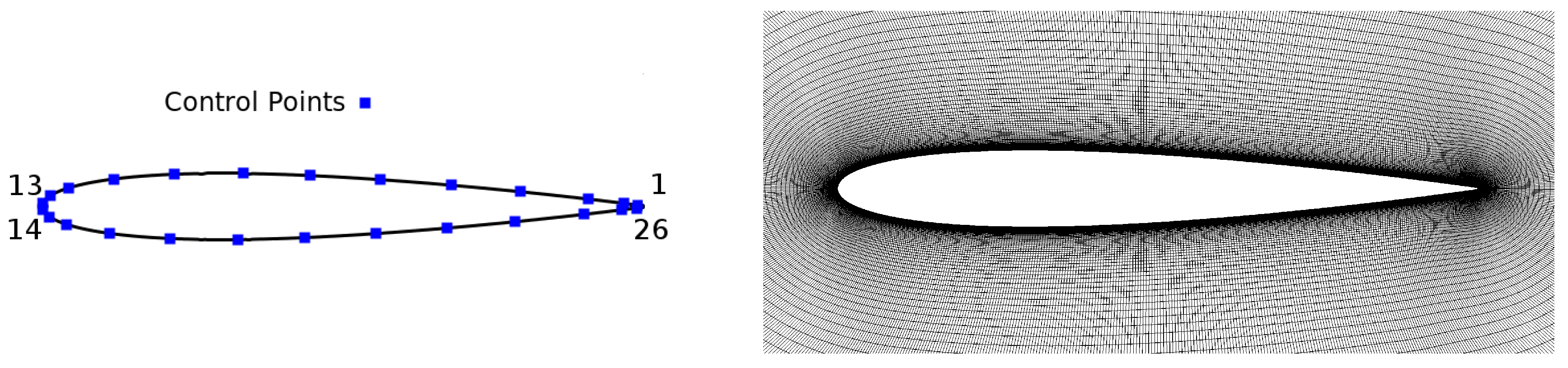
Figure 3 shows a NACA 0012 and the 26 control points of the spline defining the airfoil shape, where 13 points are on the suction and pressure side, each.
The Reynolds number of the verification case is , where the flow is fully turbulent. The angle of attack (AoA) is at and the mesh consists of cells in total, with 800 faces on the airfoil. A hexahedral O-mesh is used and the domain has a radius of 45 chord lengths. The dimensionless wall distance is at in order to fully resolve the flow in the boundary layer and Figure 3 shows a close-up view of the mesh near the airfoil.
For the sake of brevity, a mesh independency study for this angle of attack and at , as well as a validation with experimental results by Ladson [41], is presented in Appendix A.
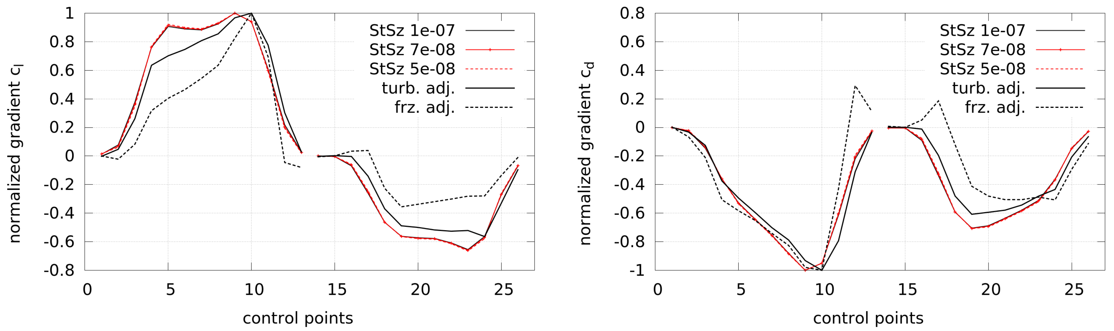
The resulting gradients via the adjoint approach as in Equation (10) and by finite differences are shown in Figure 4 along the indices of the control points (labeled as in Figure 3). The objectives are the lift coefficient and, respectively, the drag coefficient . A step size study was done by using different step sizes for the computation of finite differences, which is presented in Appendix B. The step sizes with nearly no change in the gradients, representing optimal sizes in order to avoid round-off and truncation errors, were found to be between and . The gradients are computed with respect to the point motion in a normal direction. Using the adjoint approach, they are computed by the frozen turbulence assumption and by using the adjoint turbulence model, respectively.
The gradients are scaled in order to enable a better comparison, which is done for both the adjoint gradients and the gradients by finite differences (Kim et al. [42] showed that the step size can influence the size of the gradients, which could result from the non-linear nature of the Navier–Stokes equations). In general, it can be seen that the gradients using adjoint turbulence follow the trend of the finite differences better than the frozen turbulence approach, where some gradients even have a wrong sign. Still, a deviation is visible between the reference gradients by finite differences (FDs) and the adjoint gradients, which could possibly result from the complex flow due to high turbulence near the trailing edge.
However, it can be concluded that the implementation of the adjoint turbulence model leads to a better representation of the reference gradients than the frozen turbulence assumption. Further, it is not clear how the differences between these two approaches affect the optimization processes, which is the focus of this work and will be shown in the following section.
3.6. Inverse Design
The optimizations in this work are gradient-based without any stochastic elements and can only find local optima [1,2,6]. This means that very different initial shapes converge to different optima, whereas more similar shapes converge to the same, but local, optimum (unless only one single optimum, the global one, exists). The adjoint approach is used for the gradient computation as previously discussed, and in order to increase the speed of the optimization process a quasi-Newton method is used, which approximates second-order derivatives. Here, the BFGS algorithm by Broyden, Fletcher, Goldfarb and Shanno [2] is used for updating the Hessian and the described set-up for the gradient computation is combined with the optimization module from SciPy [43], based on the programming language Python. This module offers a high flexibility for various applications and makes it easy to switch between different optimization algorithms or procedures.
All optimizations are unconstrained single-point optimizations for the lift and drag coefficients, respectively. In order to reach a certain lift coefficient or drag coefficient , the objective functions are formulated in a quadratic form:
where the index is used as a place holder for either the lift or the drag coefficient.
This formulation allows a clear convergence criterion of the objective function due to its convexity. In contrast, a pure maximization of lift or pure minimization of drag without any constraints or bounds is less suitable, since it would strongly depend on the number of control points and the mesh deformation would probably limit the process at some point, leading to wrong solutions of the primal flow field. Thus, the quadratic form of Equation (14) is used.
Although the posed optimization problem is unconstrained, it already gives insight into the effect of frozen and adjoint turbulence, as will be shown in the following section. Depending on the number of design parameters, the problem in Equation (14) may result in many possible solutions. However, for a gradient-based optimization with small shape deformations it is expected that the possible optima are close to each other. Furthermore, the resulting shapes indicate the distribution of the gradients, and thus give valuable information about the optimization process.
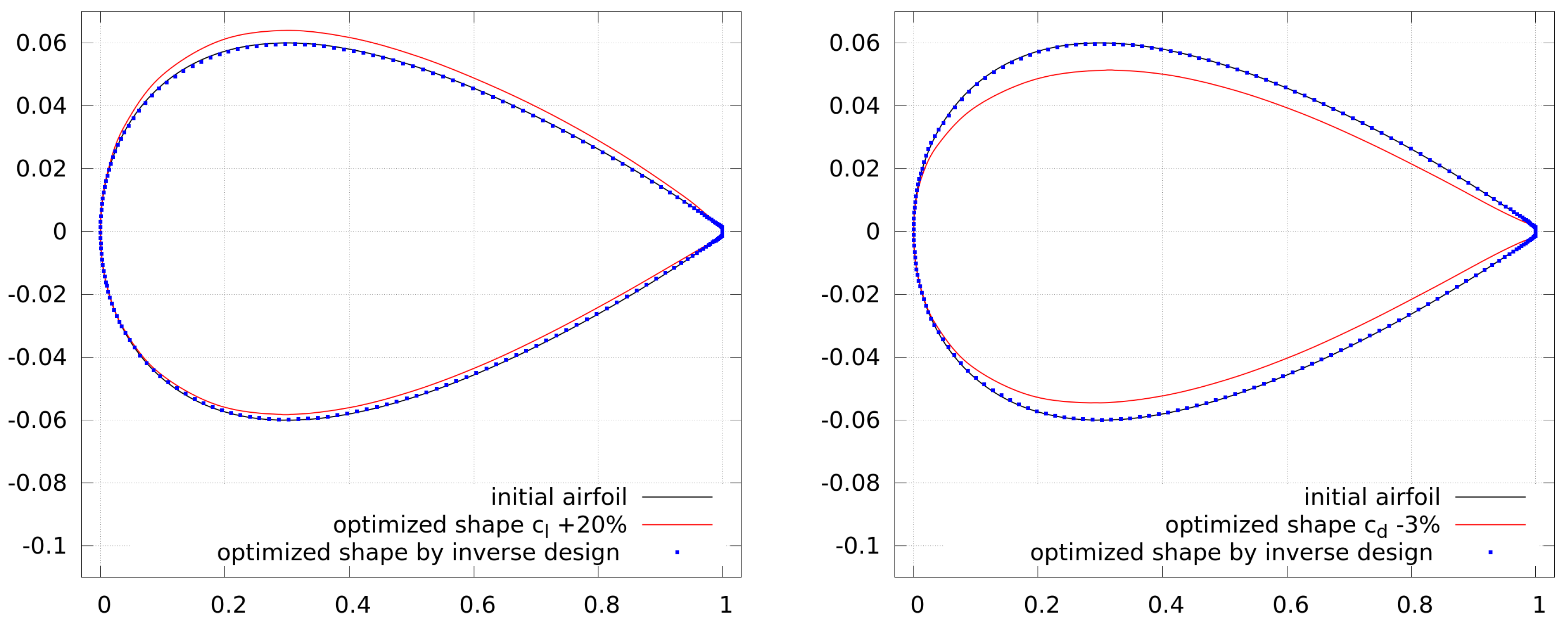
In order to provide a proof of concept of the optimization framework, a simple inverse study is conducted, where a known optimal geometry is reproduced.
The same mesh and geometry as in the previous gradient verification are used, again at and . Adjoint turbulence is used, and the airfoil is represented by a spline with 30 control points. First, the lift of the NACA 0012 is increased by . Then, this geometry is optimized such that the aim is the lift coefficient of the initial NACA airfoil. The same procedure is followed for a drag optimization, where the initial NACA 0012 is optimized for a drag decrease of .
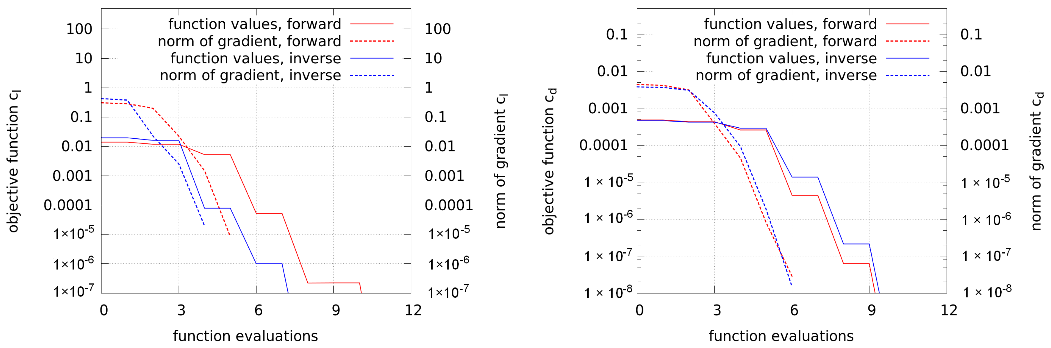
The history of function values of forward and inverse design are shown in Figure 5 for the lift and drag objectives, respectively. Also in the same plot, the supremum norm of the gradient is shown and it can be seen that all optimizations converge well. During the optimization, the flow and adjoint equations are converged to residuals of at least and , respectively. First, the RANS equations are converged, then the adjoints are computed based on the solved RANS field, and afterwards the gradient information or function value is transferred to the optimizer. With this information, the mesh is moved accordingly, but not during the solution process of the primal or adjoint fields. This procedure is also used in the following optimizations.
Figure 6 shows the initial and corresponding optimized shapes of forward and inverse design. It can be seen that the initial NACA 0012 can be reproduced by the inverse design and thus, the optimization procedure works as expected.
4. Optimization of Airfoils
In the following optimizations, the design parameters are the coordinates of the spline control points, which are equally distributed along the airfoil. The trailing edge is fixed and the splines are parametrized by 20, 30, and 50 control points (abbreviated by “cp”) in order to investigate their effect on the optimization process. As in the previous inverse design study, the optimizations aim at certain lift or drag coefficients, respectively, and the objective functions are formulated as in Equation (14). The flow solutions in the optimizations are pre-converged and the compared cases have the same level of pre-convergence.
4.1. NACA 0012 at
The initial airfoil for the first comparisons is the NACA 0012 at a Reynolds number of and an angle of attack of . The mesh and general set-up are the same as for the verification of the adjoint gradients and the inverse design of the previous section. Different numbers of spline control points are used.
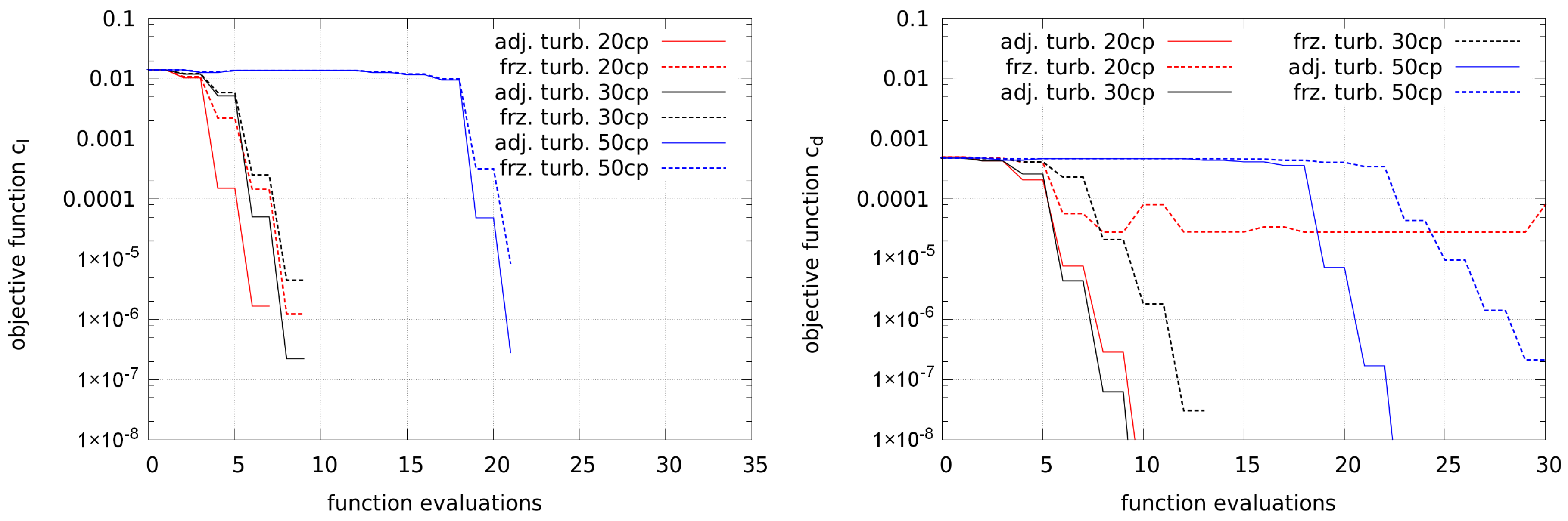
Figure 7 shows the convergence of the lift and drag optimizations. The objective for the lift is an increase of the lift coefficient by . The lift optimizations all lead to a convergent solution. More control points (labeled as “XXcp”) require more function evaluations.
The objective of the drag optimizations is a decrease of the drag coefficient by . Most cases lead to a convergent solution and only the case with frozen turbulence and 20 control points does not converge well. In order to investigate this, the gradients of the first optimization steps are plotted in Figure 8. In order to be able to compare the gradients with a different amount of control points, the gradients by 20 and 50 control points are scaled in the x-direction to match the gradients by 30 control points.
Different conclusions can be drawn from the graph. Firstly, the size of the gradients depends on the number of control points. This follows from the summation during the projection from higher to lower-dimensional space (see Equation (13)) and fewer control points need to include more information of the gradients. Secondly, the gradients obtained by frozen turbulence are smaller than the ones by adjoint turbulence. Thirdly, compared to the highest values by 20 control points and adjoint turbulence, the use of frozen turbulence leads to slightly stronger gradients near the trailing edge (at low and high numbering of control points, respectively). This results into a different shape at the trailing edge, as shown in Figure 9 (see the shape with 20 cp and frozen turbulence), where the solution of the flow as well as the adjoints may be wrong and the optimizer is not able to generate a clearly better shape from this point.
4.2. NACA 0012 at
As a next step, the angle of attack is increased to , which is closer to the stall, and flow separation becomes more dominant. The mesh and general set-up are the same as before. Since the initial lift and drag coefficients at this angle are much higher than in the previous case, an increase in lift by only and a decrease in drag by only is aimed for.
Figure 10 shows the convergence of the lift and drag optimization using the same nomenclature as before. For the lift objective, it can be seen that the cases using adjoint turbulence converge well, but the cases with frozen turbulence do not converge at all.
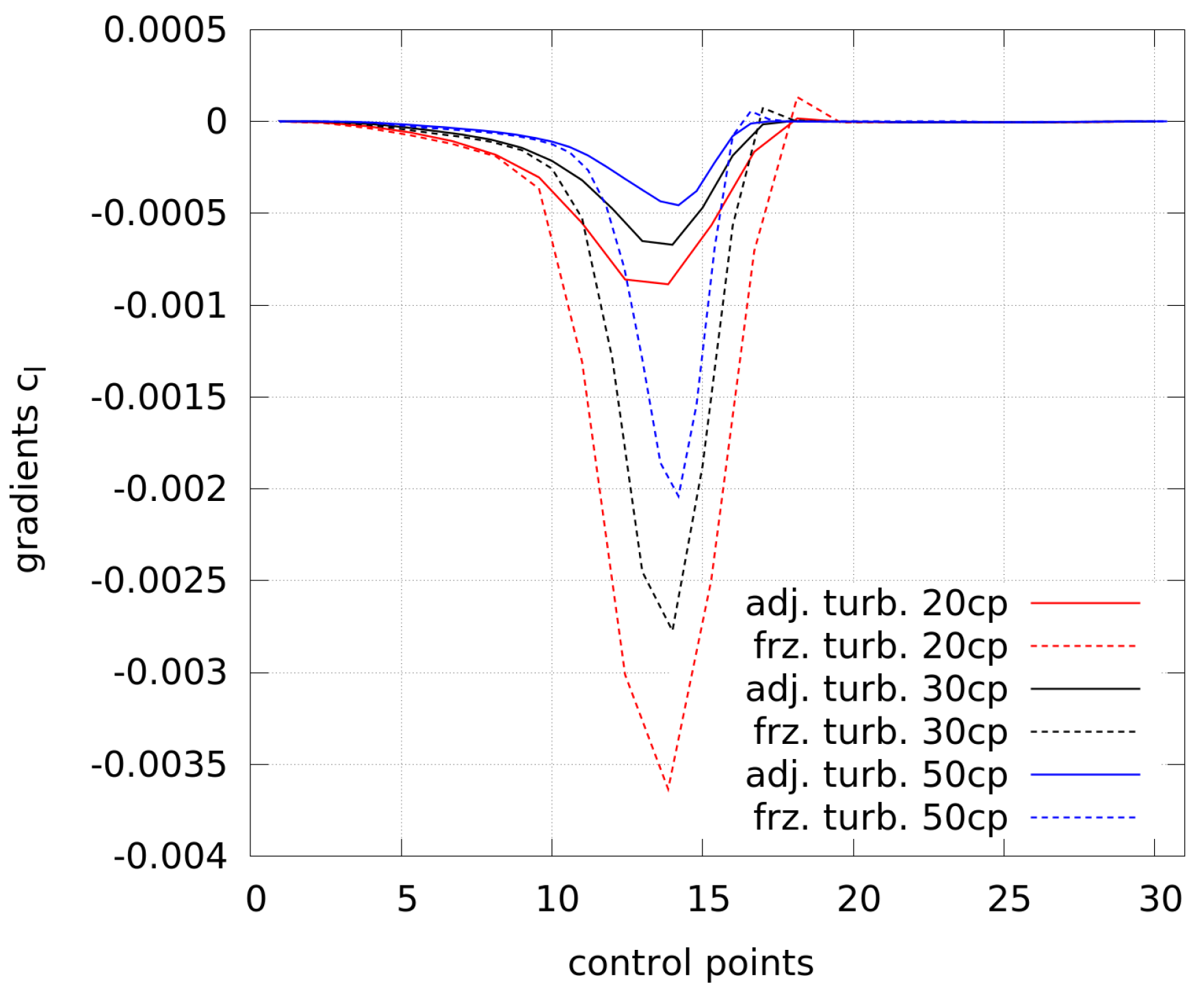
The reason for this poorer behavior using frozen turbulence can be found in the gradients shown in Figure 11, where the gradients of the first optimization step are plotted. Again, in order to be able to compare the gradients with a different number of control points, the gradients by 20 and 50 control points are scaled in the x-direction to match the gradients by 30 control points.
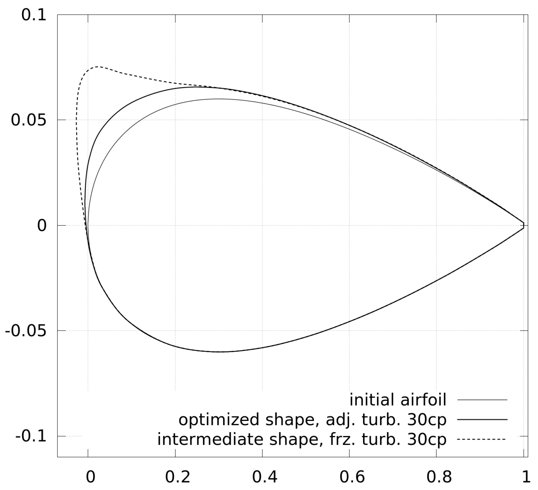
As before, due to the summation during the projection of gradients (see Equation (13)), the gradients with more design variables are smaller than the ones with fewer design variables. Besides, it can be seen that the gradients obtained by frozen turbulence are clearly bigger than the ones computed by adjoint turbulence, and show a deviating trend. These stronger gradients appear near the leading edge on the suction side and lead to a larger deformation at this part of the airfoil, which is shown in Figure 12 for an intermediate step with 30 control points and frozen turbulence.
The intermediate shape shows a stronger deformation of the leading edge on the suction side and with this shape, the adjoint equations do not properly converge, which leads to even worse gradient information afterwards. The optimization cannot recover from this and it explains the poor convergence of the optimization processes using frozen turbulence in Figure 10.
Figure 10 also shows the convergence of the drag optimization and it can be seen that the cases using adjoint turbulence converge better than the cases using frozen turbulence, where some do not converge at all. Still, the distinction is not as clear as for the lift optimization. There is a stronger dependence on the number of design variables, which may result from a higher sensitivity of the drag coefficient on the mesh motion and a higher influence of friction forces. Also, this comparison shows that a drag optimization at this angle of attack with early beginning of flow separation seems to be more challenging than the previous cases. The deviation of gradients obtained by the adjoint approach from gradients by finite differences, presented in Section 3.5, leads to this problem, which can follow from the simplifications discussed in Section 3.3. However, these are required for stable convergence of the adjoint system, which cannot be simply solved by using finer meshes.
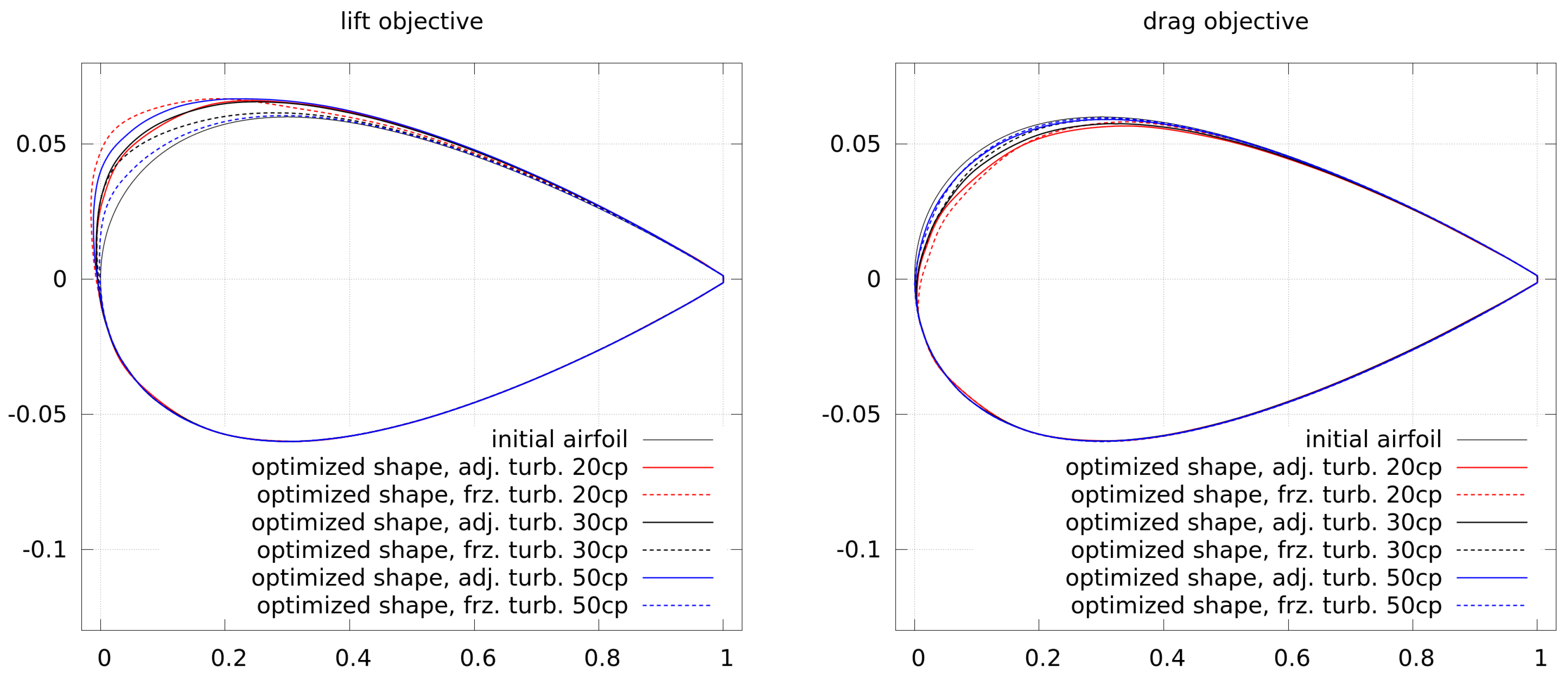
Figure 13 shows the final shapes from the lift and drag optimization at . For the lift, it can be seen that the shapes using adjoint turbulence are similar, whereas the shapes using frozen turbulence all differ from each other, which is a result of the wrong initial and following gradients. For the drag optimization, the shapes are all a little different from each other. Since the drag has a higher sensitivity to the shape, even small differences lead to a relatively strong impact on the objective function.
It can be concluded that in more complex cases (an increased angle of attack is more complex because of the beginning of separation) the use of adjoint turbulence is beneficial and leads to a better convergence behavior than in cases when frozen turbulence is used. The negative influence of the frozen turbulence assumption could become even worse when constraints are used in multi-objective optimization or more precise approximations of the Hessians are needed.
4.3. DU 93-W-210 at
The following comparison uses a wind turbine airfoil DU 93-W-210 developed at TU Delft by Timmer and van Rooij [44]. It is specially designed for the use on wind turbines and has a stronger camber as well as a higher thickness () than the previous shape. It is aerodynamically optimized for a high lift-to-drag ratio, which makes the airfoil an interesting object for optimization. The general set-up of the simulations is as before, the mesh has the same size and quality, and the Reynolds number is again . The angle of attack is at , where this airfoil has a higher lift and drag than the previous NACA airfoil. Thus, the objective is to increase the lift coefficient by only and to decrease the drag by .
Figure 14 shows the convergence of the lift and drag optimization, where the convergence of frozen and adjoint turbulence is very similar. Only in the case of 50 control points is a clearly higher number of function evaluations required, which may result from more steps in order to compute the approximated Hessian, and this case does not scale linearly.
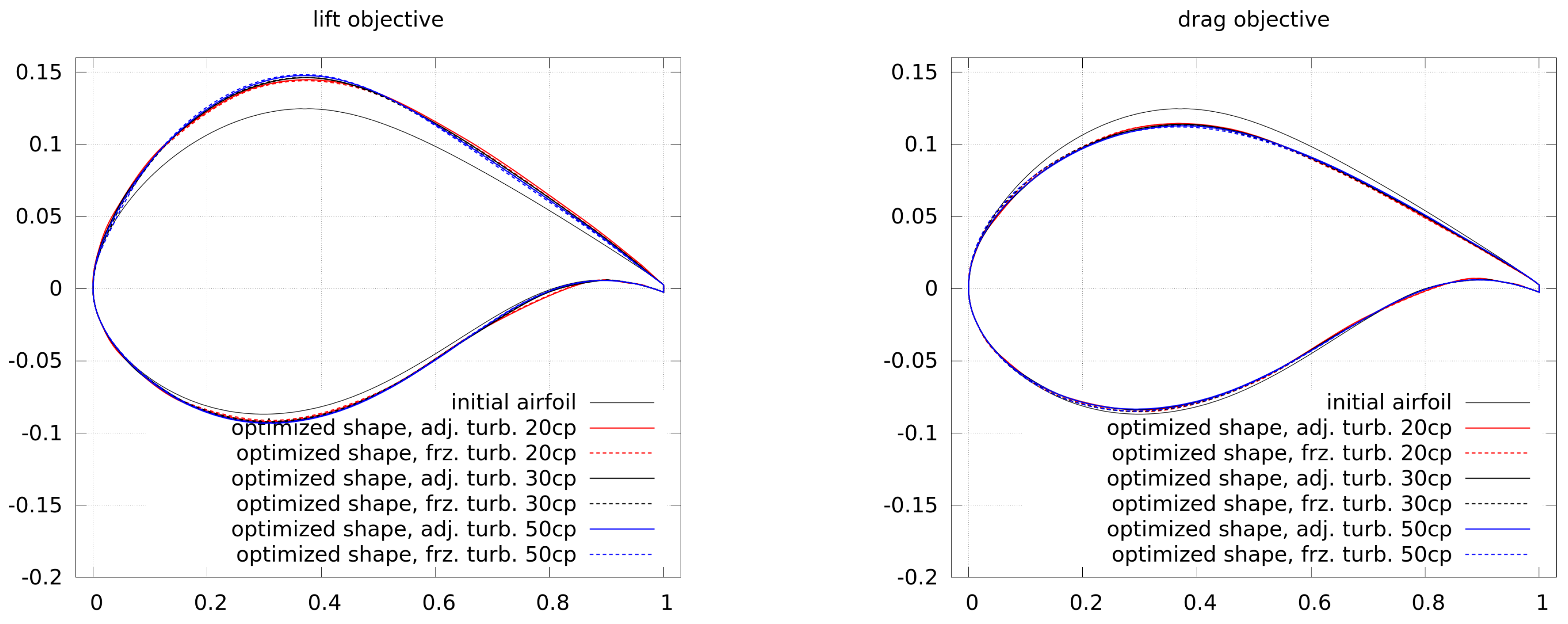
The final shapes of the lift and drag optimizations are shown in Figure 15. The higher lift is gained by an increase in camber and thickness. The differences between shapes generated by adjoint and frozen turbulence are small. The lower drag is gained by a decrease in camber and thickness. Again, the differences between shapes generated by adjoint and frozen turbulence are small.
4.4. DU 93-W-210 at
Due to a different curvature and thickness, the DU 93-W-210 has different aerodynamic characteristics than the symmetric NACA airfoil. The lift of the DU airfoil drops less strongly in the stall, but the airfoil stalls a few degrees earlier. That is why the following optimizations are conducted at , which is little before the stall in fully-turbulent flow. The objectives are an increase in lift by and a decrease in drag by .
Figure 16 shows the convergence of the lift and drag optimization, where the convergence of frozen and adjoint turbulence is similar.
As in the previous case, at a lower angle of attack, the use of 50 control points requires a higher number of CFD iterations. This may result from more steps in order to compute the approximated Hessian and does not scale linearly.
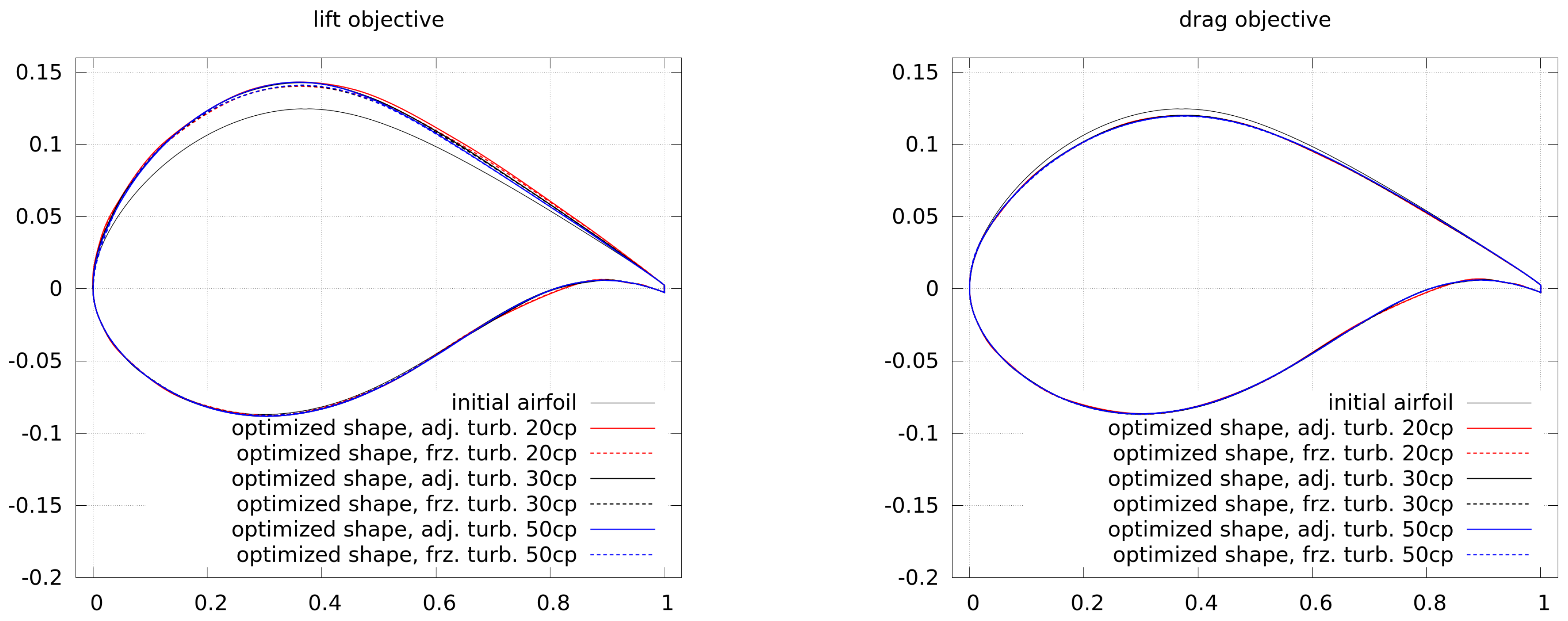
The final shapes of the lift and drag optimizations are shown in Figure 17. The higher lift is gained through an increase in camber and thickness. The lower drag is gained by a decrease in camber and thickness. As for the lower angle of attack, the differences between shapes generated by using adjoint and frozen turbulence are small.
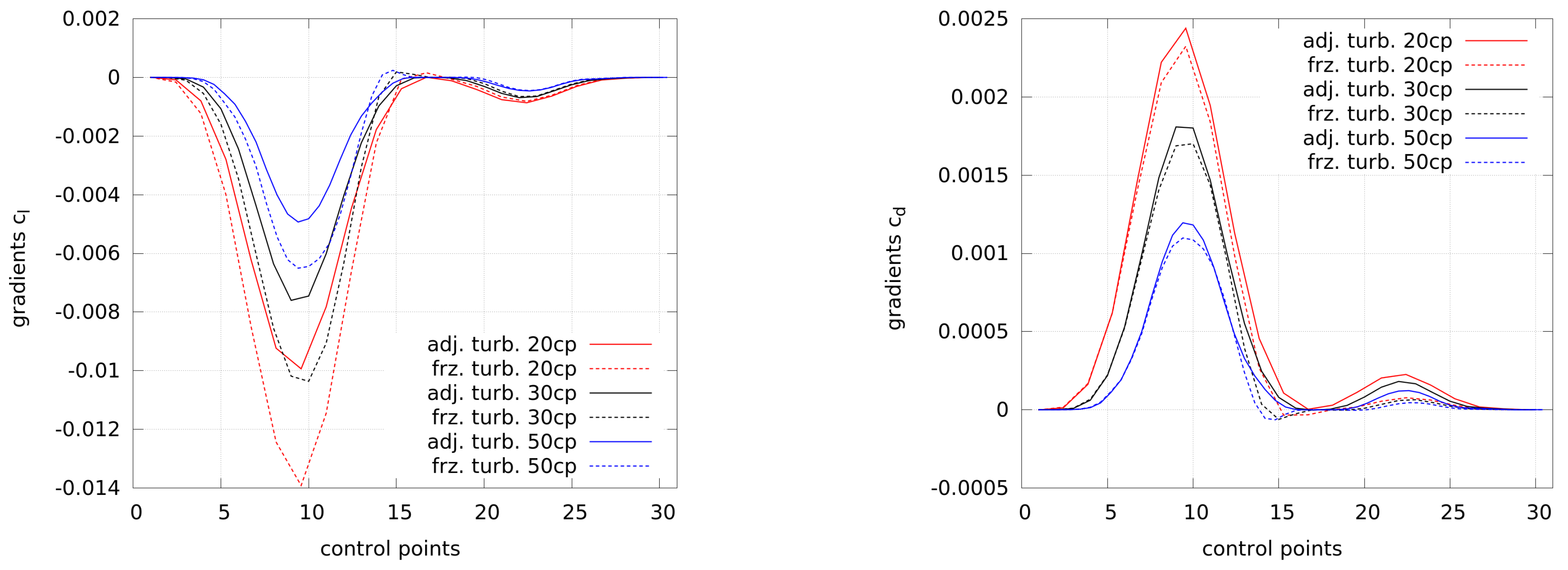
In order to investigate why the differences between frozen and adjoint turbulence are small in terms of convergence and shape, Figure 18 shows the gradients of the first optimization step for lift and drag objective, respectively. For the sake of a better comparison of the gradients using different numbers of control points, the abscissa is scaled to match 30 control points. Beside minor differences, it can be seen that the gradients are of similar size and show a similar trend. Although the gradients by frozen turbulence are a little larger than the ones by adjoint turbulence, the optimization processes are not influenced much. This is very different to the previous optimizations of the symmetric NACA airfoil and results from the different airfoil shapes. The shape of the DU airfoil leads to gradients which are the strongest on the central suction side. Thus, mainly thickness and camber are changed during the optimization, which has a positive effect on the convergence of the optimization. In contrast, the symmetric NACA airfoil has stronger gradients near the leading edge (especially at ) and subsequently, the leading edge is more strongly deformed and the use of adjoint turbulence is more important.
5. Summary and Conclusions
Airfoil shape optimization based on CFD and the adjoint approach is already an established method used by several authors. In this study, the effect of the so-called “frozen turbulence” assumption in incompressible flows is compared with the adjoints to a turbulence model, here the Spalart–Allmaras model. The simulations were conducted with the open-source CFD code OpenFOAM-2.3.0, which was extended by the authors for the presented purposes, i.e., external aerodynamics and the corresponding gradient computations as well as a robust, but precise mesh deformation. The implemented mesh motion technique is particularly suitable for shape deformations of airfoils, preserving the high mesh quality in the boundary layer. The solution procedure of the adjoint equations was improved in terms of stability and speed. The convergence time was reduced by half using the SIMPLEC algorithm. The objective functions of the single-point optimizations were quadratic functions in order to reach a certain target lift or drag coefficient, respectively. The function and gradient evaluations were coupled with the optimization module SciPy, written in the programming language Python. Unconstrained quasi-Newton optimizations were used, where the Hessian was approximated by a BFGS update.
The airfoils in the optimizations were represented by splines using different numbers of control points. In some cases, the convergence of the optimization and the resulting shapes depended on the number of control points, and it is recommended that at least 30 spline control points are used.
The presented cases showed that the adjoint turbulence is not always necessary, since some optimizations converged well with gradients obtained by the frozen turbulence approach. This strongly depends on the case itself and for some cases (which may be considered relatively simple), the significant effort for implementing or deriving an adjoint turbulence model can be saved. Besides, the additional PDE from the adjoint turbulence model leads to a higher computational time, which was roughly twice the time needed with frozen turbulence. The reader may evaluate this individually for his or her problem his- or herself, but in general, it is recommended that adjoints to the turbulence model be used, if available. In many cases it is useful, and in some even inevitable, as some airfoil shapes in complex flows may not be optimized without adjoint turbulence. This necessity may increase when a different optimizer is selected in order to use constraints and when the approximation of the Hessian has to be more precise. Noise in the gradients will be amplified using second-order derivatives, which leads to poorer convergence or even complete failure of the optimization.
Since unconstrained optimizations were conducted, other aerodynamic measures or thickness were not included in the optimization objectives, but thickness was clearly changed in the presented cases. Fulfilling the objective function, the shapes are mathematically correct, but for many engineering purposes they may not be useful. This can be considered as a negative side-effect of the presented single-objective optimization. Thickness or other aerodynamic constraints are important for many airfoil applications, e.g., in wind turbines, and hence, they shall be included in future work.
Acknowledgments
The authors would like to thank Martin Bünner (NTB, University of Applied Sciences Buchs, Switzerland) and Lena Vorspel (ForWind, University of Oldenburg, Germany) for the fruitful discussions about optimization and the adjoint approach. The authors appreciate the financial support of the project WIMS–Cluster (0324005), funded by the Federal Ministry of Economic Affairs and Energy, following a decision of the German Bundestag. The simulations were performed at the HPC Cluster EDDY, located at the University of Oldenburg (Germany) and funded by the Federal Ministry for Economic Affairs and Energy (Bundesministeriums für Wirtschaft und Energie) under grant number 0324005.
Author Contributions
M.S. performed the simulations and wrote the paper; B.S. and J.P. supervised the work, analyzed the data, and contributed to the general interpretation of the results.
Conflicts of Interest
The authors declare no conflict of interest.
Appendix A
A mesh study is conducted for a NACA 0012 at and two angles of attack: and . The Spalart–Allmaras turbulence model is used and in order to fully resolve the flow in the boundary layer the dimensionless wall distance is at . The domains have a radius of 45 chord lengths and are spatially discretized as shown in Table A1. Hexahedral O-meshes are used and in order to be able to use these meshes for the computation of adjoint equations, they are finer than necessary for standard flow solutions with RANS.

Table A1.
Number of cells used in the mesh study.
| Cells Around Airfoil | Cells in Radial Direction | Cells in Total | |
|---|---|---|---|
| coarse mesh | 400 | 130 | 52,000 |
| medium mesh | 800 | 260 | 208,000 |
| fine mesh | 1,600 | 520 | 832,000 |
The resulting changes in lift and drag coefficients are shown in the following Table A2, where the relative differences are computed based on the results of the finest mesh.
Table A2.
Relative differences , in (%) of lift and drag coefficients compared to the coefficients resulting from the finest mesh.
Table A2.
Relative differences , in (%) of lift and drag coefficients compared to the coefficients resulting from the finest mesh.
| coarse mesh | ||||
| medium mesh | ||||
| fine mesh | ||||
Comparing the medium and the fine mesh, the differences at are below and only for the drag at , which is already near stall, the difference is above . The medium mesh represents a compromise between mesh independency and fast primal and adjoint solutions, and as such is used within this work.
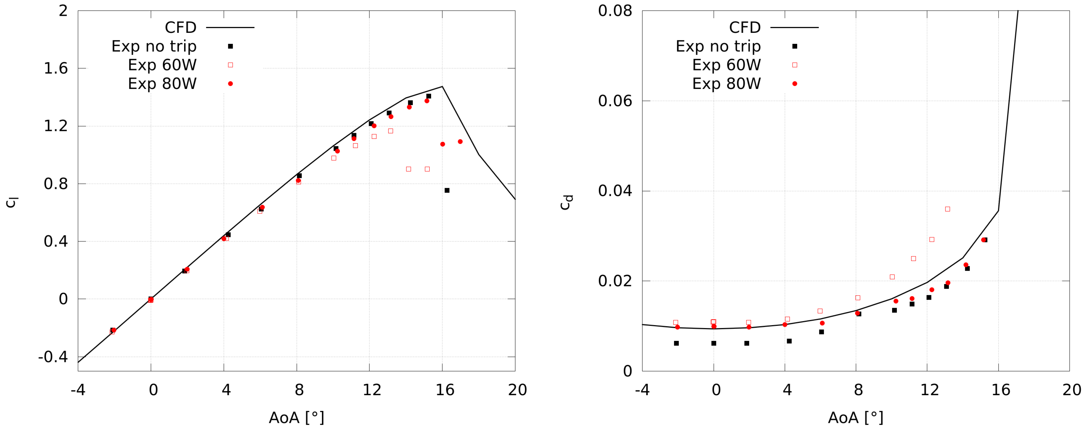
With this mesh for the NACA 0012, a validation is done at , comparing experimental results from Ladson [41] with the numerical predictions. Again, the simulations were conducted to be fully-turbulent with the Spalart–Allmaras model without transition. In the measurements, different levels of roughness are used and beside a clean configuration, boundary layer tripping is also used. The carborundum strips were placed at of the chord on the suction and pressure side and had different grit sizes: 60-W and 80-W.
The resulting validation of the lift and drag coefficients is shown in Figure A1. In general, the CFD is able to reproduce the measurements, although the deep stall shows some deviations, which is a common effect from 2D-RANS simulations, but 3D wind tunnel measurements. Since the focus of this work is not a validation of OpenFOAM, but an investigation of frozen and adjoint turbulence, these results are considered to be good enough.
Figure A1.
Validation of lift and drag coefficients of a NACA 0012 at (experimental results by Ladson [41]).
Figure A1.
Validation of lift and drag coefficients of a NACA 0012 at (experimental results by Ladson [41]).
Appendix B
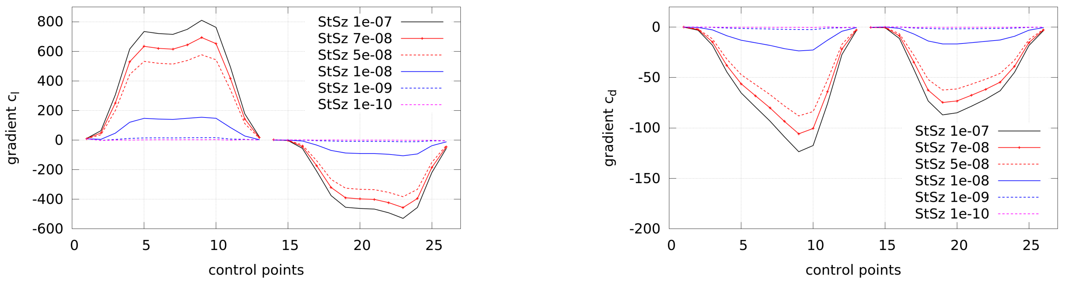
A step size study for computing finite differences is conducted for the NACA airfoil at and . The airfoil is represented by a spline with 26 control points and different step sizes are used in order to search for an optimal range, where neither round-off errors nor truncation errors appear.
The resulting gradients are plotted in Figure A2 along the indices of the control points (labeled as in Figure 3) and it can be seen that the smallest changes in gradients are between and . Still, the gradients are not exactly the same and a promising approach to avoid the step size problem of finite differences is the complex step method [40]. However, this is not in the scope of this work, since the objectives in the optimizations are fulfilled when using adjoint turbulence. The complex step method may be used in the future for a better verification of the adjoint implementation when more complex objective functions are used, which require a higher accuracy of the gradients.
Figure A2.
Gradients obtained by finite differences (FDs) for lift objective (“gradient ”) and drag objective (“gradient ”). Different step sizes (StSz) are used for finite differencing.
Figure A2.
Gradients obtained by finite differences (FDs) for lift objective (“gradient ”) and drag objective (“gradient ”). Different step sizes (StSz) are used for finite differencing.
Appendix C
The derivation of the adjoints to the Spalart–Allmaras turbulence model follows the description of Zymaris et al. [15]. However, our own derivation led to minor differences and for the sake of brevity only the finally resulting equations are shown here.
The adjoint momentum equation including adjoint turbulent viscosity is:
where the derivatives and directly result from the Spalart–Allmaras model:
The adjoint continuity equation is:
The equation for the adjoint eddy-viscosity is:
where again some derivatives and directly result from the Spalart–Allmaras model:
Standard Dirichlet and zero Neumann boundary conditions are used for the far-field boundaries, where the adjoint BCs are opposite to the primal BCs.
References
- Arora, J.S. Introduction to Optimum Design, 2nd ed.; Elsevier Academic Press: Cambridge, MA, USA, 2004. [Google Scholar]
- Nocedal, J.; Wright, S.J. Numerical Optimization, 2nd ed.; Springer Science+Business Media: Berlin, Germany, 2006. [Google Scholar]
- Jameson, A.; Martinelli, L. Optimum Aerodynamic Design Using the Navier-Stokes Equations. Theor. Comput. Fluid Dyn. 1998, 10, 213–237. [Google Scholar] [CrossRef]
- Giles, M.B.; Pierce, N.A. An Introduction to the Adjoint Approach to Design. In Flow, Turbulence and Combustion; Kluwer Academic Publishers: Dordrecht, the Netherlands, 2000; Volume 65, pp. 393–415. [Google Scholar]
- Papoutsis-Kiachagias, E.M.; Giannakoglou, K.C. Continuous Ajoint Methods for Turbulent Flows, Applied to Shape and Topology Optimization: Industrial Applications. Arch. Comput. Methods Eng. 2014, 23, 255–299. [Google Scholar] [CrossRef]
- Thévenin, D.; Janiga, G. Optimization and Computational Fluid Dynamics; Springer: Berlin/Heidelberg, Germany, 2008. [Google Scholar]
- Nadarajah, S.K.; Jameson, A. A Comparison of the Continuous and Discrete Adjoint Approach to Automatic Aerodynamic Optimization. Can. J. Earth Sci. 2000, 43, 1445–1466. [Google Scholar]
- Carnarius, A.; Thiele, F.; Özkaya, E.; Nemili, A.; Gauger, N. Optimal Control of Unsteady Flows Using a Discrete and a Continuous Adjoint Approach. In Proceedings of the 25th System Modeling and Optimization (CSMO), Berlin, Germany, 12–16 September 2011. [Google Scholar]
- Othmer, C. A continuous adjoint formulation for the computation of topological and surface sensitivities of ducted flows. Int. J. Numer. Methods Fluids Wiley InterSci. 2008. [Google Scholar] [CrossRef]
- Anderson, W.K.; Bonhaus, D.L. Airfoil Design on Unstructured Grids for Turbulent Flows. AIAA J. 1999, 37, 185–191. [Google Scholar] [CrossRef]
- Nielsen, E.J.; Anderson, W.K. Aerodynamic Design Optimization on Unstructured Meshes Using the Navier-Stokes Equations. AIAA J. 1999, 37, 1411–1419. [Google Scholar] [CrossRef]
- Lyu, Z.; Kenway, G.K.W.; Paige, C.; Martins, J.R.R.A. Automatic Differentiation Adjoint of the Reynolds-Averaged Navier-Stokes Equations with a Turbulence Model. In Proceedings of the 21st AIAA Computational Fluid Dynamics Conference, San Diego, CA, USA, 24–27 June 2013. [Google Scholar]
- Osusky, L.; Buckley, H.; Reist, T.; Zingg, D.W. Drag Minimization Based on the Navier–Stokes Equations Using a Newton-Krylov Approach. AIAA J. 2015, 53, 1555–1577. [Google Scholar] [CrossRef]
- Dwight, R.; Brezillon, J. Effect of various approximations of the discrete adjoint on gradient-based optimization. AIAA J. 2006, 44, 3022–3031. [Google Scholar] [CrossRef]
- Zymaris, A.S.; Papadimitriou, D.I.; Giannakoglou, K.C.; Othmer, C. Continuous adjoint approach to the Spalart-Allmaras turbulence model for incompressible flows. Comput. Fluids 2009, 38, 1528–1538. [Google Scholar] [CrossRef]
- Spalart, P.R.; Allmaras, S.R. A one-equation turbulence model for aerodynamic flows. In Proceedings of the 30th Aerospace Sciences Meeting and Exhibit, Reno, NV, USA, 6–9 January 1992. [Google Scholar]
- Bueno-Orovio, A.; Castro, C.; Palacios, F.; Zuazua, E. Continuous Adjoint Approach for the Spalart-Allmaras Model in Aerodynamic Optimization. AIAA J. 2012, 50. [Google Scholar] [CrossRef]
- Kavvadias, I.S.; Papoutsis-Kiachagias, E.M.; Dimitrakopoulos, G.; Giannakoglou, K.C. The continuous adjoint approach to the k-ω SST turbulence model with applications in shape optimization. Eng. Optim. Taylor Francis Group 2014, 47. [Google Scholar] [CrossRef]
- OpenCFD. OpenFOAM®—The Open Source Computational Fluid Dynamics (CFD) Toolbox. Available online: www.OpenFOAM.org (accessed on 19 January 2018).
- Towara, M.; Naumann, U. A Discrete Adjoint Model for OpenFOAM. Proced. Comput. Sci. 2013, 18, 429–438. [Google Scholar] [CrossRef]
- Önder, A. Active Control of Turbulent Axisymmetric Jets Using Zero-Net-Mass-Flux Actuation. Ph.D. Thesis, Katholieke Universiteit Leuven, Leuven, Belgium, 2014. [Google Scholar]
- Petropoulou, S. Industrial Optimisation Solutions based on OpenFOAM Technology. In Proceedings of the 5th European Conference on Computational Fluid Dynamics (ECCOMAS), Lisbon, Portugal, 14–17 June 2010. [Google Scholar]
- Othmer, C.; de Villier, E.; Weller, H. Implementation of a continuous adjoint for topology optimization of ducted flows. In Proceedings of the 18th AIAA Computational Fluid Dynamics Conference, Miami, FL, USA, 25–28 June 2007. [Google Scholar]
- Jameson, A.; Reuther, J. Control Theory Based Airfoil Design using the Euler Equations. In Proceedings of the 5th Symposium on Multidisciplinary Analysis and Optimization, Panama City Beach, FL, USA, 7–9 September 1994. [Google Scholar]
- Castro, C.; Lozano, C.; Palacios, F.; Zuazua, E. Systematic Continuous Adjoint Approach to Viscous Aerodynamic Design on Unstructured Grids. AIAA J. 2007, 45, 2125–2139. [Google Scholar] [CrossRef]
- Mohammadi, B.; Pironneau, O. Shape Optimization in Fluid Mechanics. Ann. Rev. Fluid Mech. 2004, 36, 255–279. [Google Scholar] [CrossRef]
- Soto, O.; Löhner, R. On the computation of flow sensitivities from boundary integrals. In Proceedings of the 42nd AIAA Aerospace Sciences Meeting and Exhibit, Reno, NV, USA, 5–8 January 2004. [Google Scholar]
- Choi, H.; Hinze, M.; Kunisch, K. Instantaneous control of backward-facing step flows. Appl. Numer. Math. 1999, 31, 133–158. [Google Scholar] [CrossRef]
- Stück, A. Adjoint Navier-Stokes Methods for Hydrodynamic Shape Optimisation. Ph.D. Thesis, Technische Universität Hamburg-Harburg, Hamburg, Germany, 2012. [Google Scholar]
- Palacios, F.; Alonso, J.J.; Jameson, A. Design of free-surface interfaces using RANS equations. In Proceedings of the 43rd Fluid Dynamics Conference, San Diego, CA, USA, 24–27 June 2013. [Google Scholar]
- Patankar, S.V. Numerical Heat Transfer and Fluid Flow; Hemisphere Publishing Corporation: Washington, DC, USA, 1980. [Google Scholar]
- Van Doormaal, J.P.; Raithby, G.D. Enhancements of the SIMPLE method for predicting incompressible fluid flows. Numer. Heat Transf. 1984, 7, 147–163. [Google Scholar] [CrossRef]
- Hojjat, M. Node-Based Parametrization for Shape Optimal Design. Ph.D. Thesis, Technische Universität München, Munich, Germany, 2015. [Google Scholar]
- Jameson, A.; Vassber, J.C. Studies of alternative numerical optimization methods applied to the brachistochrone problem. Comput. Fluid Dyn. J. 2000, 9, 281–296. [Google Scholar]
- Soto, O.; Löhner, R.; Yang, C. A stabilized pseudo-shell approach for surface parametrization in CFD design problems. Commun. Numer. Methods Eng. 2002, 18, 251–258. [Google Scholar] [CrossRef]
- Kropatsch, W.; Kampel, M.; Hanbury, A. Computer Analysis of Images and Patterns—12th International Conference, CAIP 2007, Proceedings; Springer: Berlin Heidelberg, 2007. [Google Scholar]
- Anderson, W.K.; Venkatakrishnan, V. Aerodynamic design optimization on unstructured grids with a continuous adjoint formulation. In Proceedings of the 35th Aerospace Sciences Meeting and Exhibit, Reno, NV, USA, 6–9 January 1997. [Google Scholar]
- Lozano, C. Discrete surprises in the computation of sensitivities from boundary integrals in the continuous adjoint approach to inviscid aerodynamic shape optimization. Comput. Fluids 2012, 56, 118–127. [Google Scholar] [CrossRef]
- Schramm, M.; Stoevesandt, B.; Peinke, J. Simulation and Optimization of an Airfoil with Leading Edge Slat. J. Phys. Conf. Ser. 2016, 753, 022052. [Google Scholar] [CrossRef]
- Martins, J.R.R.A.; Kroo, I.M.; Alonso, J.J. An Automated Method for Sensitivity Analysis using Complex Variables. In Proceedings of the 38th AIAA Aerospace Sciences Meeting, Reno, NV, USA, 10–13 January 2000. [Google Scholar]
- Ladson, C.L. Effects of Independent Variation of Mach and Reynolds Numbers on the Low-Speed Aerodynamic Characteristics of the NACA 0012 Airfoil Section; NACA Technical Memorandum; NASA: Washington, DC, USA, 1988; Volume 4074.
- Kim, S.; Alonso, J.J.; Jameson, A. A Gradient Accuracy Study for the Adjoint-Based Navier-Stokes Design Method. In Proceedings of the 37th AIAA Aerospace Sciences Meeting, Reno, NV, USA, 11–14 January 1999. [Google Scholar]
- SciPy. Scientific Computing Tools for Python. Available online: www.SciPy.org (accessed on 19 January 2018).
- Timmer, W.A.; van Rooij, R.P.J.O.M. Summary of the Delft University Wind Turbine Dedicated Airfoils. In Proceedings of the 41st Aerospace Sciences Meeting and Exhibit, Reno, NV, USA, 6–9 January 2003. [Google Scholar]
Figure 1.
Example spline from the airfoil to the far field with interpolation factor .
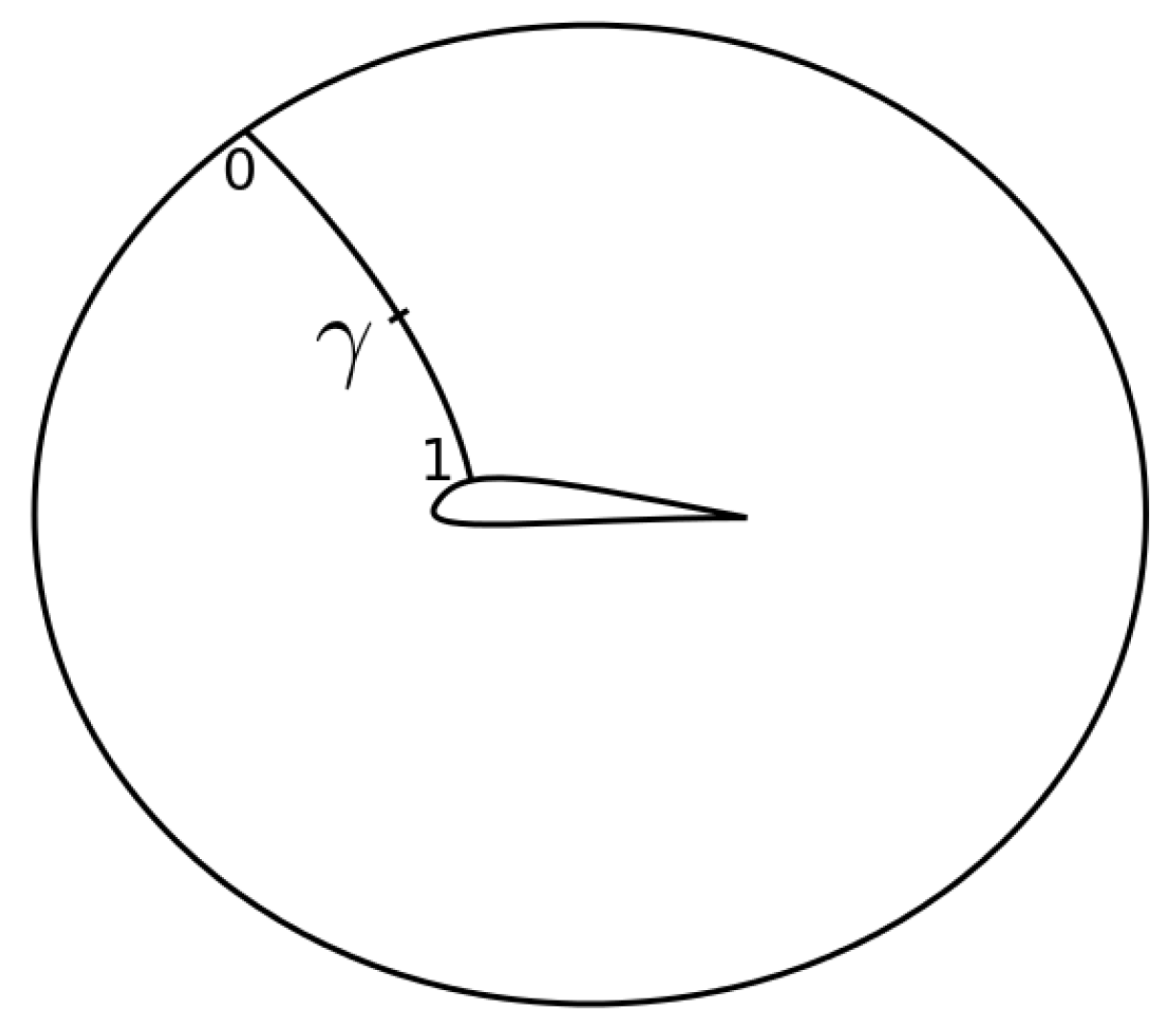
Figure 2.
Mesh deformation of the suction side of an airfoil.

Figure 3.
Control points of the verification case and close-up view of the mesh near the airfoil.

Figure 4.
Comparisons of gradients obtained by finite differences (FsD) and gradients via the adjoint approach for lift objective (“gradient ”) and drag objective (“gradient ”). Different step sizes (StSz) are used for finite differencing. Adjoint and frozen turbulence are used for gradients via the adjoint approach (labeled as “adj. turb” and “frz. turb”, respectively).

Figure 5.
Objective functions as in Equation (14) and norm of the gradient for the lift objective and drag objective along the number of function evaluations.
Figure 5.
Objective functions as in Equation (14) and norm of the gradient for the lift objective and drag objective along the number of function evaluations.

Figure 6.
Shapes of inverse design study for the lift objective and drag objective. For a better visualization of the inverse design, only every third point is plotted.
Figure 6.
Shapes of inverse design study for the lift objective and drag objective. For a better visualization of the inverse design, only every third point is plotted.

Figure 7.
Objective functions for lift and drag as in Equation (14) along the number of function evaluations for the NACA 0012 at . Frozen as well as adjoint turbulence are used. The number of control points is labeled as “XXcp”.
Figure 7.
Objective functions for lift and drag as in Equation (14) along the number of function evaluations for the NACA 0012 at . Frozen as well as adjoint turbulence are used. The number of control points is labeled as “XXcp”.

Figure 8.
Gradients of the first optimization step for a decrease in drag by at . Frozen as well as adjoint turbulence are used. The number of control points is labeled as “XXcp”. The control points start from the trailing edge on the suction side, pass the leading edge, and end at the trailing edge on the pressure side.
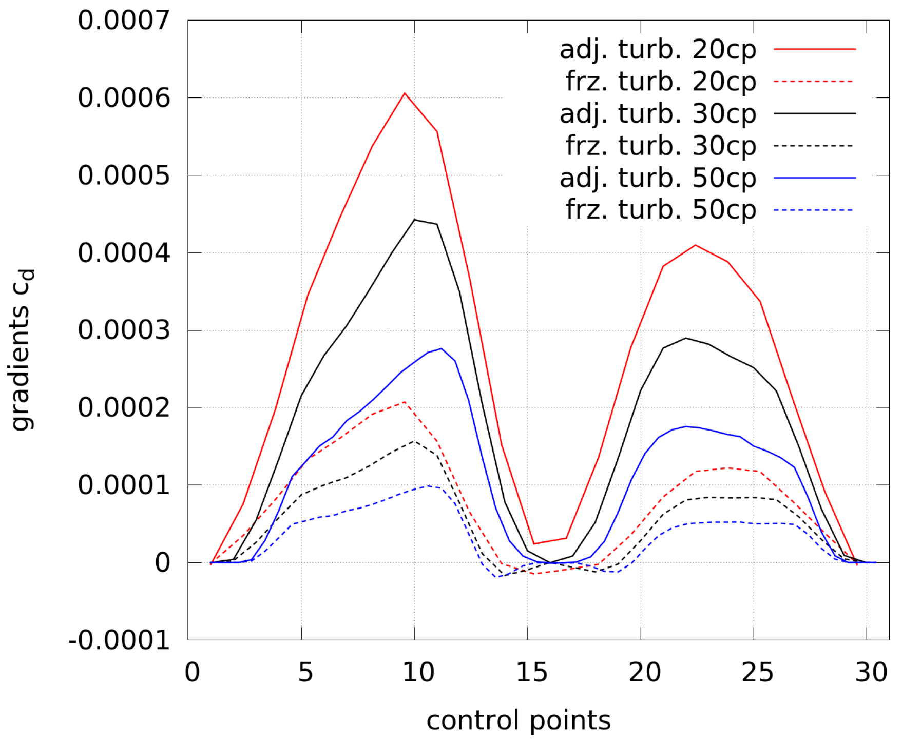
Figure 9.
Airfoil shapes using adjoint and frozen turbulence for the NACA 0012 at . The objective is a decrease in drag by . Frozen as well as adjoint turbulence are used. The number of control points is labeled as “XXcp”.
Figure 9.
Airfoil shapes using adjoint and frozen turbulence for the NACA 0012 at . The objective is a decrease in drag by . Frozen as well as adjoint turbulence are used. The number of control points is labeled as “XXcp”.
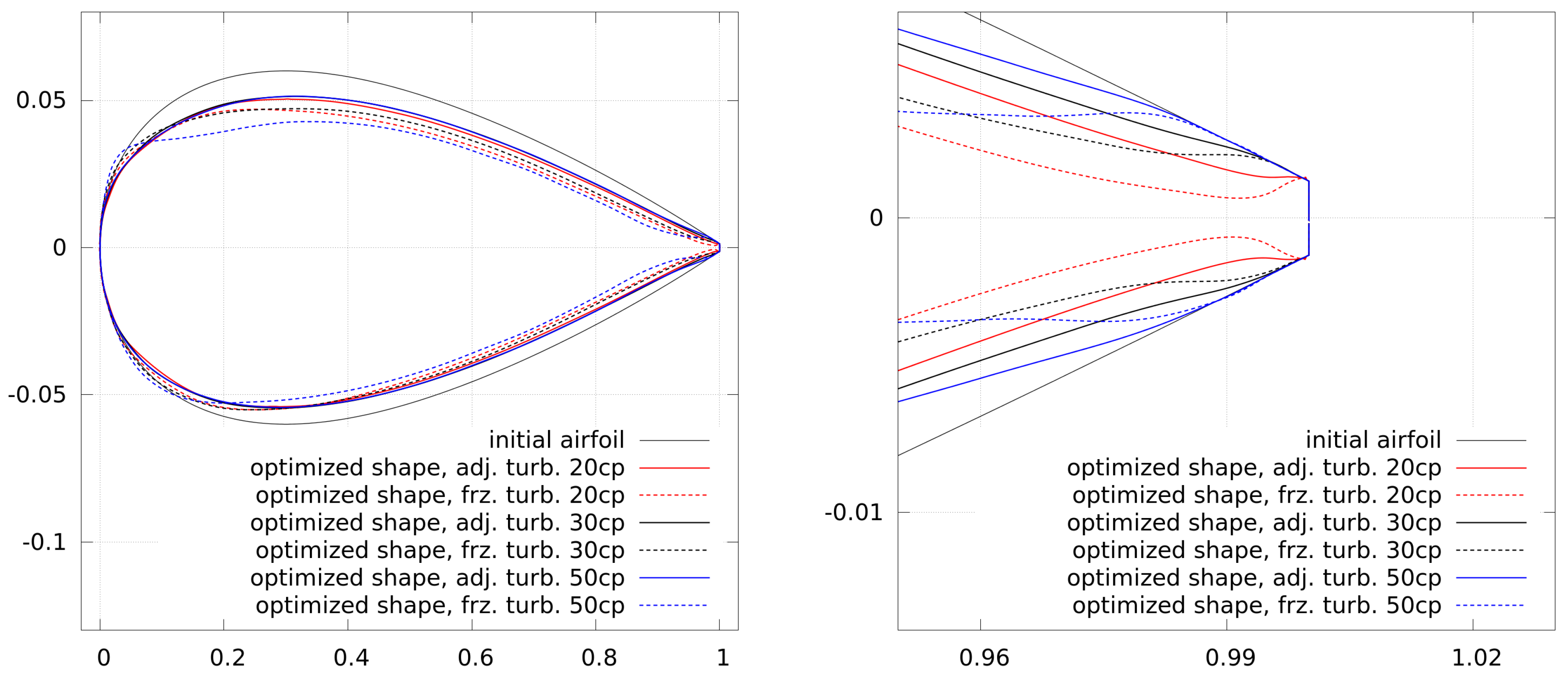
Figure 10.
Objective functions for lift and drag as in Equation (14) along the number of function evaluations for the NACA 0012 at . Frozen as well as adjoint turbulence are used. The number of control points is labeled as “XXcp”.
Figure 10.
Objective functions for lift and drag as in Equation (14) along the number of function evaluations for the NACA 0012 at . Frozen as well as adjoint turbulence are used. The number of control points is labeled as “XXcp”.
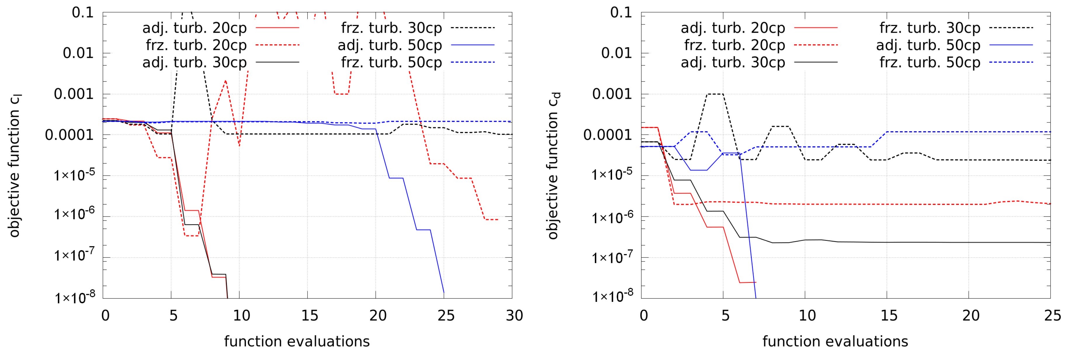
Figure 11.
Gradients of the first optimization step for an increase in lift by at . Frozen as well as adjoint turbulence are used. The number of control points is labeled as “XXcp”. The control points start from the trailing edge on the suction side, pass the leading edge, and end at the trailing edge on the pressure side.

Figure 12.
Intermediate airfoil shape during an optimization of lift at using frozen turbulence compared to the initial airfoil and the final shape using adjoint turbulence (all with 30 control points).
Figure 12.
Intermediate airfoil shape during an optimization of lift at using frozen turbulence compared to the initial airfoil and the final shape using adjoint turbulence (all with 30 control points).

Figure 13.
Airfoil shapes using adjoint and frozen turbulence for the lift and drag objective with NACA 0012 at . Frozen as well as adjoint turbulence are used. The number of control points is labeled as “XXcp”.
Figure 13.
Airfoil shapes using adjoint and frozen turbulence for the lift and drag objective with NACA 0012 at . Frozen as well as adjoint turbulence are used. The number of control points is labeled as “XXcp”.

Figure 14.
Objective functions for lift and drag as in Equation (14) along the number of function evaluations for the DU 93-W-210 at . Frozen as well as adjoint turbulence is used. The number of control points is labeled as “XXcp”.
Figure 14.
Objective functions for lift and drag as in Equation (14) along the number of function evaluations for the DU 93-W-210 at . Frozen as well as adjoint turbulence is used. The number of control points is labeled as “XXcp”.
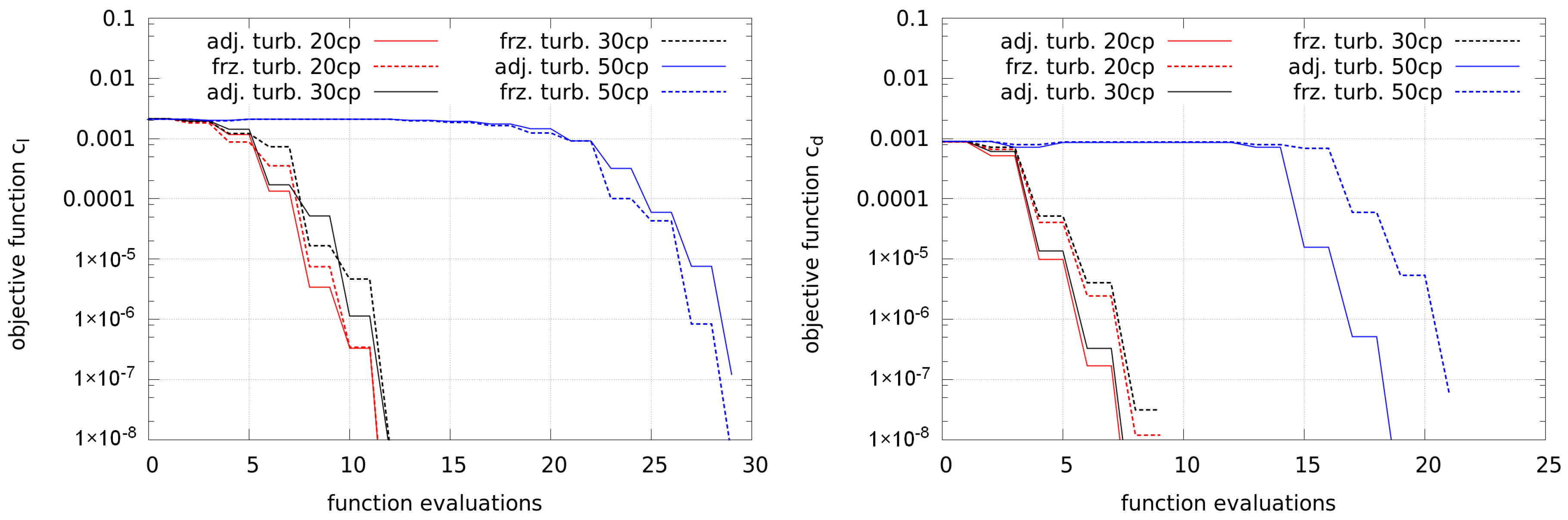
Figure 15.
Airfoil shapes using adjoint and frozen turbulence for the lift and drag objective for DU 93-W-210 at . Frozen as well as adjoint turbulence are used. The number of control points is labeled as “XXcp”.
Figure 15.
Airfoil shapes using adjoint and frozen turbulence for the lift and drag objective for DU 93-W-210 at . Frozen as well as adjoint turbulence are used. The number of control points is labeled as “XXcp”.

Figure 16.
Objective functions for lift and drag as in Equation (14) along the number of function evaluations for the DU 93-W-210 at . Frozen as well as adjoint turbulence are used. The number of control points is labeled as “XXcp”.
Figure 16.
Objective functions for lift and drag as in Equation (14) along the number of function evaluations for the DU 93-W-210 at . Frozen as well as adjoint turbulence are used. The number of control points is labeled as “XXcp”.
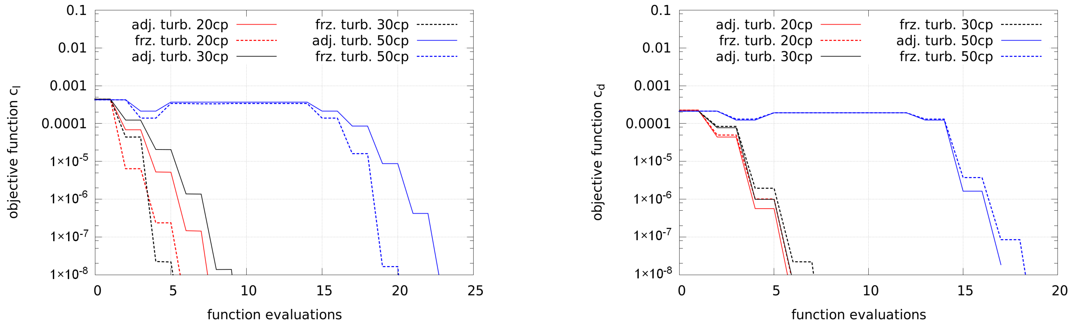
Figure 17.
Airfoil shapes using adjoint and frozen turbulence for the lift and drag objective for DU 93-W-210 at . Frozen as well as adjoint turbulence are used. The number of control points is labeled as “XXcp”.
Figure 17.
Airfoil shapes using adjoint and frozen turbulence for the lift and drag objective for DU 93-W-210 at . Frozen as well as adjoint turbulence are used. The number of control points is labeled as “XXcp”.

Figure 18.
Gradients of the first optimization step for lift and drag objective of the DU 93-W-210 at . Frozen as well as adjoint turbulence are used. The number of control points is labeled as “XXcp”. The control points start from the trailing edge on the suction side, pass the leading edge and end at the trailing edge on the pressure side.

© 2018 by the authors. Licensee MDPI, Basel, Switzerland. This article is an open access article distributed under the terms and conditions of the Creative Commons Attribution (CC BY) license (http://creativecommons.org/licenses/by/4.0/).
Share and Cite
MDPI and ACS Style
Schramm, M.; Stoevesandt, B.; Peinke, J. Optimization of Airfoils Using the Adjoint Approach and the Influence of Adjoint Turbulent Viscosity. Computation 2018, 6, 5. https://doi.org/10.3390/computation6010005
AMA Style
Schramm M, Stoevesandt B, Peinke J. Optimization of Airfoils Using the Adjoint Approach and the Influence of Adjoint Turbulent Viscosity. Computation. 2018; 6(1):5. https://doi.org/10.3390/computation6010005
Chicago/Turabian StyleSchramm, Matthias, Bernhard Stoevesandt, and Joachim Peinke. 2018. "Optimization of Airfoils Using the Adjoint Approach and the Influence of Adjoint Turbulent Viscosity" Computation 6, no. 1: 5. https://doi.org/10.3390/computation6010005
Note that from the first issue of 2016, this journal uses article numbers instead of page numbers. See further details here.