Temporal Variation of the Pressure from a Steady Impinging Jet Model of Dry Microburst-Like Wind Using URANS


1
School of Mechanical and Aerospace Engineering, Nanyang Technological University, 50 Nanyang Avenue, Singapore 639798, Singapore
2
Energy Research Institute (ERI@N), 1 CleanTech Loop, #06-04, CleanTech One, Singapore 637141, Singapore
*
Author to whom correspondence should be addressed.
Computation 2018, 6(1), 2; https://doi.org/10.3390/computation6010002
Submission received: 16 November 2017
/
Revised: 20 December 2017
/
Accepted: 28 December 2017
/
Published: 5 January 2018
(This article belongs to the Special Issue Computational Methods in Wind Engineering)
Abstract
:The objective of this study is to investigate the temporal behavior of the pressure field of a stationary dry microburst-like wind phenomenon utilizing Unsteady Reynolds-averaged Navier-Stokes (URANS) numerical simulations. Using an axisymmetric steady impinging jet model, the dry microburst-like wind is simulated from the initial release of a steady downdraft flow, till the time after the primary vortices have fully convected out of the stagnation region. The validated URANS results presented herein shed light on the temporal variation of the pressure field which is in agreement with the qualitative description obtained from field measurements. The results have an impact on understanding the wind load on structures from the initial touch-down phase of the downdraft from a microburst. The investigation is based on CFD techniques, together with a simple impinging jet model that does not include any microphysical processes. Unlike previous investigations, this study focuses on the transient pressure field from a downdraft without obstacles.
1. Introduction
A thunderstorm downburst is an intense transient downdraft of air that induces an outburst of damaging wind on or near the surface of the Earth. Fujita [1] classified a downburst as “microburst” when the outflow extends less than along the Earth’s surface, and “macroburst” when the outflow reaches more than . Microbursts are also further classified as of dry or wet type. Dry microbursts are formed in deep, dry, and well-mixed atmospheric boundary layers, while wet microbursts are formed together with thunderstorm clouds with shallow, well-mixed boundary layers and large vertical gradients of potential energy [2]. The formation of downbursts begins with convection driving updrafts, which transport warm, moist, and more buoyant air to great height. The onset of downdrafts occurs when there is cooling of air by the evaporation of rain and melting of ice, causing the air density in the evaporation and melting regions to increase. The colder and denser air accelerates vertically downward from the cloud base. Difference in density between the downdraft and the surrounding atmosphere subsequently leads to the entrainment of the surrounding atmospheric air into the downdraft core, resulting in ring vortices due to Kelvin-Helmholtz instability (KHI). The behaviour of KHI is governed by Taylor-Goldstein equation. The KHI occurs when Richardson () number is below 0.25. Ri is a dimensionless number measuring the buoyancy effect to the inertia force effect. Fujita [1] reported that the scales of the full-scale downbursts are such that the diameter of the inlet of a full-scale downburst at the cloud base level is between and , and the extreme wind event typically lasts from 5 to 30 min. The range of height () of the downburst cloud measured from the cloud base to the surface of the Earth usually falls within , where is the diameter of the downdraft at the level of the cloud base [3]. In passing, it is noted that the term micro in this context refers to very different scales when compared to those in microfluidics where downburst due to temperature gradients has also been studied [4].
Early studies of downburst wind shear were motivated by aviation accidents. There were numerous field studies conducted to capture the downburst wind in nature. Examples of field studies are: Northern Illinois Meteorological Research on Downbursts (NIMROD) [5], Joint Airport Weather Studies (JAWS) [6], the Federal Aviation Administrative Lincoln Laboratory Operational Weather Studies (FLOWS) [7], the Thunderstorm Wind Project in Singapore [8], the European Project “Wind and Ports” [9,10,11], project SCOUT [12], and the “forensic study of the Lubbock-Reese downdraft of 2002” [13].
The downburst wind shear near the Earth’s surface is of great interest to wind engineers as the outflow exerts wind forces that may pose catastrophic failure risk to structures and buildings, which are typically designed according to wind-loading industry codes (International Electrotechnical Commission 2005). This is highlighted by many recent investigations during the last few decades [14,15,16,17,18,19,20,21,22]. The dry microburst-like wind near the ground surface is the scope of the present study. Hjelmfelt [3] and Choi [8] have proven in laboratories that the round impinging jets can be used to emulate the outflow near the ground surface because the mean radial field of the flow near the ground agreed reasonably well with one of the field measurements, particularly the time-averaged peak radial velocity. Apart from the impinging jet, other models, such as the ‘cooling source’ approach, as proposed by Anderson et al. [23] and meteorological full or sub-cloud modelling techniques, as demonstrated by Orf et al. [24,25,26] and Vermeire et al. [27], have been used previously to emulate downburst wind shear in laboratories, or in numerical simulations. The benefits of the impinging jet modelling approach, when compared to the other approaches, is a much lower computational cost and its ability to model the macro dynamics of downburst [28]. Note that a steady impinging jet model does not have the same meteorological processes (i.e., density stratification of the atmosphere and buoyancy-induced turbulence), transient behaviour and Reynolds number observed in a real full-scale microburst. However, it has been observed by Hjelmfelt [3] that the characteristics of a steady impinging-jet flow are akin to the major features in a 10-min transient microburst event at its maximum strength at the near-surface region. Moreover, the impinging jet has been widely utilized by many researchers to model the microburst’s outburst-flow profiles. Even though there is a significant scale difference between an impinging jet model and a real microburst, the impinging jet flow is able to reveal the flow characteristics of a microburst-like wind and wind load acting on structures if the Reynolds number is above the order of , as demonstrated by Xu and Hangan [29]. The open literature has reported many researchers who have conducted numerical, experimental, and semi-empirical studies of a downburst using the impinging jet model. Below, we list past investigations categorized by their methodology rather than chronologically.
For numerical Computational Fluid Dynamics (CFD) studies, both unsteady and steady numerical Reynolds-averaged Navier-Stokes (URANS and RANS) simulations have been conducted by Chay et al. [30], Kim and Hangan [28], Li et al. [31] and Zhang et al. [22]. A combination of numerical and experimental work of steady impinging jet flow can be found in the work of Wood et al. [32], Sengupta and Sarkar [33], Xu and Hangan [29], and Das et al. [34]. Experimental results have been reported by Landreth and Adrian [35], Chay and Letchford [15], Choi [8], and Zhang et al. [36,37]. In addition, semi-empirical models by Oseguera and Bowles [38], Vicroy [39], Wood et al. [32], and Li et al. [40] were created to provide estimations of the microburst-like wind shear near the ground. Both the experimental results and semi-empirical models have been compared with the field measurements and they yielded reasonably good agreement.
To the authors’ knowledge, there is no literature documenting the temporal variation of the pressure field for a microburst-like wind simulated with steady impinging jet model by Unsteady Reynolds Averaged Navier-Stokes (URANS) approach. The objective is to investigate the temporal variation of the pressure field along the radial direction of the steady impinging jet model, starting from the initial release of the jet to the time when the primary vortices have exited the computational domain. Even with a stationary impinging jet, the resulting flow field is unsteady. One of the goals with the present work is to demonstrate that the standard tool for simulating unsteady flow (URANS) is able to capture the transient effects reasonably well. In addition, we show that the unsteady solution approaches the same values of the pressure, as obtained from steady simulations (RANS), which is the most utilized method in past investigations.
The RANS results that are presented here are validated with the published laboratory impinging jet data, while the URANS results are compared qualitatively with the temporal variation of the pressure observed in nature. In addition, the RANS and URANS results are shown to be consistent. The aim of the study is to improve the understanding of the wind load from the initial touch-down phase of the downdraft from a microburst. The investigation, using CFD, is dealing with an impinging jet model, which does not include any microphysical processes. This simplification of the real physics shortens the duration of simulation. Microphysical processes are usually simulated with cloud models or numerical weather prediction to provide an even higher resolution estimation of the surface wind. However, the substantial increase in the duration of simulation might not be well justified.
2. Computational Method
The commercial CFD code ANSYS Fluent 13 [41] is used to model the steady impinging jet model in the present study.
2.1. Governing Equations
For the axisymmetric steady impinging jet model used herein, the Coriolis force is not modelled due to the minor influences on the mean wind direction and height, according to Holmes [42]. The highest wind speed of downburst is about , as observed in field measurements [43] (Mach number Ma < 0.3), which would infer that the flow is essentially incompressible [21]. The wind flow satisfies the Reynolds-averaged mass and momentum conservation equations:
where is the density of the fluid, is the pressure, is the mean velocity, denotes the spatial co-ordinates, is the gravitational term and is the time quantity. The term for Reynolds stress component corresponds to , where is the fluctuating velocity component. For RANS, the first term in Equation (2) is zero.
Note that the full governing equations (Navier-Stokes) cannot be solved directly as in the turbulence investigations using much smaller geometries (see further references in, for example, the recent work by Skote [44]). Hence, the equations have been averaged, with the penalty of the unknown Reynolds stress term that needs to be modelled in terms of mean flow variables in order to close to system of equations.
The RANS approach has the flow quantities time-averaged from the start of the simulation. On the other hand, URANS is based on a smaller averaging time frame, and can capture the developing flow structures, though the smaller turbulence time-scales are not resolved.
2.2. Computational Domain, Boundary Conditions and Numerical Schemes
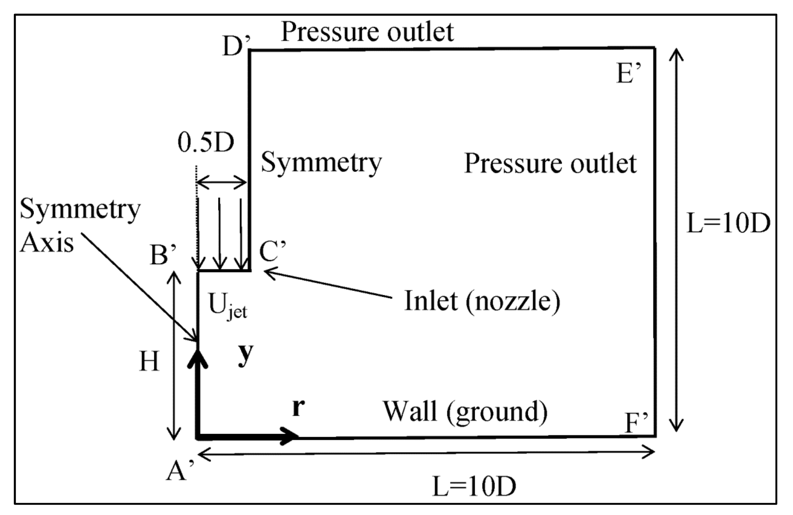
The computational domain is presented in Figure 1. There are two possible outlets (E’F’ and D’E’) in the two-dimensional (2D) axisymmetric domain shown in the figure, and each outlet should be placed at a certain distance where the outflow has attained steady-state, fully developed boundary layer with mean gauge pressure of approximately. It is also expected that there might be some backflow re-entering at these outflow boundaries as the primary vortex ring convects out of the domain. Pressure outlets are placed far away from axis (A’B’), and wall (A’F’) boundaries, respectively, to give sufficient length for flow development and to ensure that the outlets have minimal influence on the flow near the stagnation point (i.e., r/D less than 3). Boundary C’D’ is specified as ‘symmetry’ boundary, such that the flux normal to the boundary is zero. The wall (A’F’) boundary is specified as a smooth, no-slip wall, with length L = 10D.
The computational domain is packed with the uniformly distributed structured quadrilateral grids. The mesh at the wall (ground) region is strenuously refined in order to resolve the viscous laminar sub-layer and the log-law region at non-dimensionless wall distance: of order unity, because the enhanced wall treatment option in FLUENT is employed, where the is friction velocity, is the turbulent viscosity and is the wall-adjacent grid distance. The enhanced wall treatment in FLUENT is a near-wall modelling method that combines a two-layer model with enhanced wall functions and it is suitable for complex boundary layer seen in the impinging wall jet. The whole domain is subdivided into a viscosity-affected region and a fully-turbulent region. In the viscosity-affected near-wall region, the one-equation model of Wolfstein [45] is employed. In the fully turbulent outer region, the realizable k-ε turbulence [46] model is used. The turbulent viscosity is smoothly combined by a two-layer formulation approach. The law of the wall is constructed by utilizing a mathematical function proposed by Kader [47]. For the inlet (nozzle), a turbulent intensity of 1% is imposed and is taken to be hydraulic diameter required to compute turbulence quantities: turbulent kinetic energy and turbulent dissipation rate . The realizable k-ε turbulence model is tested to ensure that it is able to model the radial velocity in the impingement zone ( less than 3). Prior to any validation study, the selection of this turbulence model is solely based on the fact that it contains mathematical constraints that restrict the solution to be always physical, making it advantageous for calculating the flow around the stagnation center.
The spatial discretization schemes for k, , , and employ higher-order scheme Quadratic Upstream Interpolation for Convective Kinematics (QUICK) [48], which is 3rd-order accurate on structured uniform mesh. The pressure and momentum terms are discretized using 2nd-order upwind scheme. The 1st order discretization scheme is used only in the first 200 iterations in order to increase the rate of convergence, but the scheme is converted to QUICK and continued iterating from the intermediate solutions to final solutions. The 1st order scheme was not used to iterate to the final solution directly, due to false diffusion that gives rise to physically unrealistic final solutions [49]. For the pressure-velocity coupling, the Semi-Implicit Method for Pressure Linked Equations (SIMPLE) algorithm [50] is applied. The convergence criteria have been limited to .
An evaluation of the time step sizes for the URANS simulation was conducted and a time step size of was selected. Time is non-dimensionalised with and , and is denoted in the following. With this scaling, the time step becomes . The selected time step size has passed a time sensitivity test to ensure that it will not have any significant influence on the CFD results.
2.3. Scaling Factors of the Impinging Jet Model
The spatial scale of the full-scale downburst is derived from the field measurements of dry microburst, as observed by Hjelmfelt [3]. The diameter of a full-scale dry microburst in nature is while the smaller diameter of the impinging jet nozzle used in the present study is D = 28.7 mm. Based on this field measurement, the geometric scaling factor in the present study is of the order of .
The dry microburst observed by Fujita had a maximum velocity magnitude of about 60 m/s. The smaller inlet velocity magnitude at the impinging jet nozzle is about 10 m/s. Thus, the velocity scaling factor is about 1/6. Scaling factors calculation has also been performed previously by authors working on scale models, Mason et al. [51] and Das et al. [52], to reduce the total number of cells required when using impinging jet for downburst simulation.
The height of the downburst cloud has a base (H/D) between 0.75 and 7.5 (dimensionless) in nature, while the present impinging jet model has a nozzle height (H/D) varying between 1 and 5.
2.4. Grid Convergence
Four sets of meshes are constructed for the grid convergence study. The number of elements of a set has at least 35% more than any of the other sets. Grid resolution for all the meshes used for the present mesh convergence study are higher than any of the previously published numerical simulations [22,28,34]. Details of the meshes are summarized in Table 1.
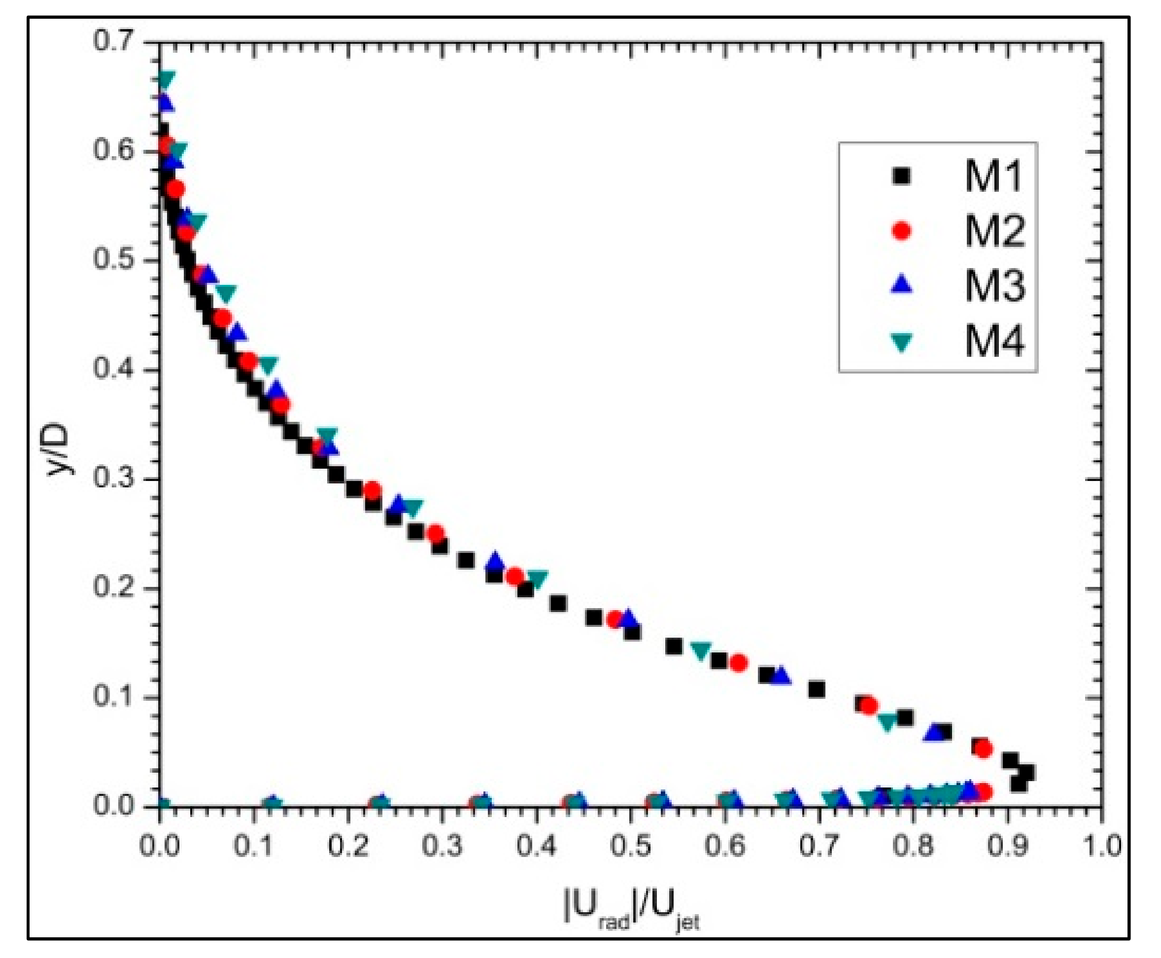
The radial velocity profiles at , produced by the realizable k-ε RANS turbulence model, are compared for the different meshes in Figure 2. All of the meshes from M1 and M4 showed that the solutions are already grid-independent. The non-dimensional wall distance varies from 0.4 to 0.6, depending on the local skin friction, and this is within the required for employing the enhanced wall function in FLUENT. M4 uses the least number of cells and is chosen for subsequent simulations.
2.5. Validation of RANS Results
The RANS CFD simulation of the round impinging jet flow will be validated with two published experimental data: Xu and Hangan [29] and Zhang [21], which we denote XH and ZG in the following. The impinging jet model used is a scale model of the full-scale downburst. The uniform velocity magnitude = 10 m/s and 100 m/s are applied at the inlet of the CFD domain, which correspond to the values in XH and ZG, respectively. Even though the inlet velocity magnitude are not the same as those that are prescribed in the two published experiments, the Reynolds numbers (Re) of the two simulations will be the same as those in the experiments (i.e., Re = 20,000 for XH, and Re = 288,046 for ZG). The diameter (D) of the jet is taken to be D = 28.7 mm and D = 41.3 mm at the inlet (nozzle), and the ratios of the height-to-ground wall surface are H/D = 2 and 4 for ZG and XH experiments, respectively (where H is the height of the nozzle).
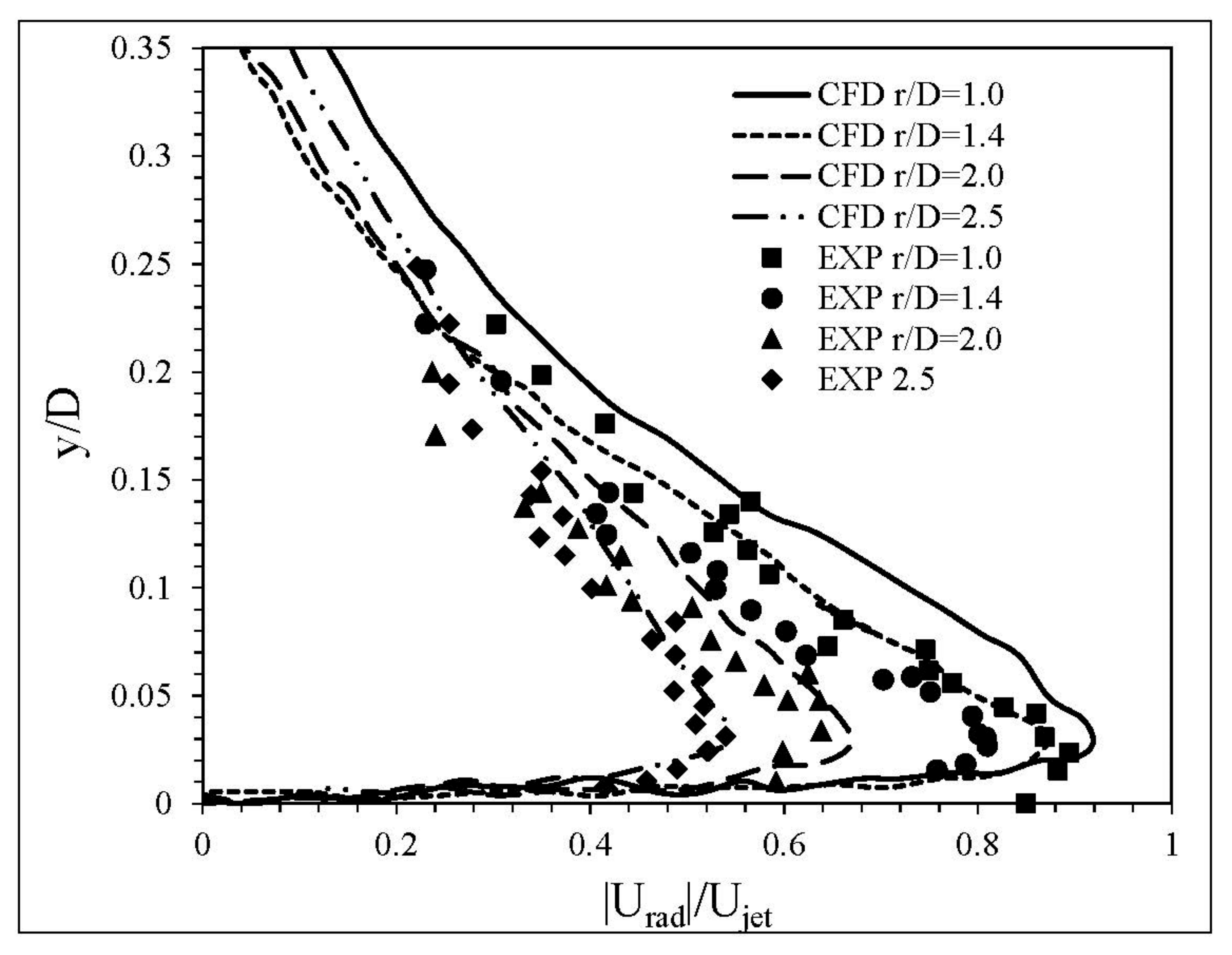
From Figure 3, the RANS results at four radial locations r/D = 1, 1.4, 2, and 2.5 show good agreement with the experimental results from XH (H/D = 4 and Re = 20,000). The slight over-prediction of the peak normalized radial velocity at respective radial locations indicates that the realizable k-ε turbulence model gives a more ‘conservative’ prediction of the peak value. The term ‘conservative’ in the present study refers to the predicted peak value being slightly higher than the experimental results. Based on the studies by Lim et al. [53], it can be inferred that an accurate prediction of the mean velocity also will produce an accurate prediction of the mean pressure.
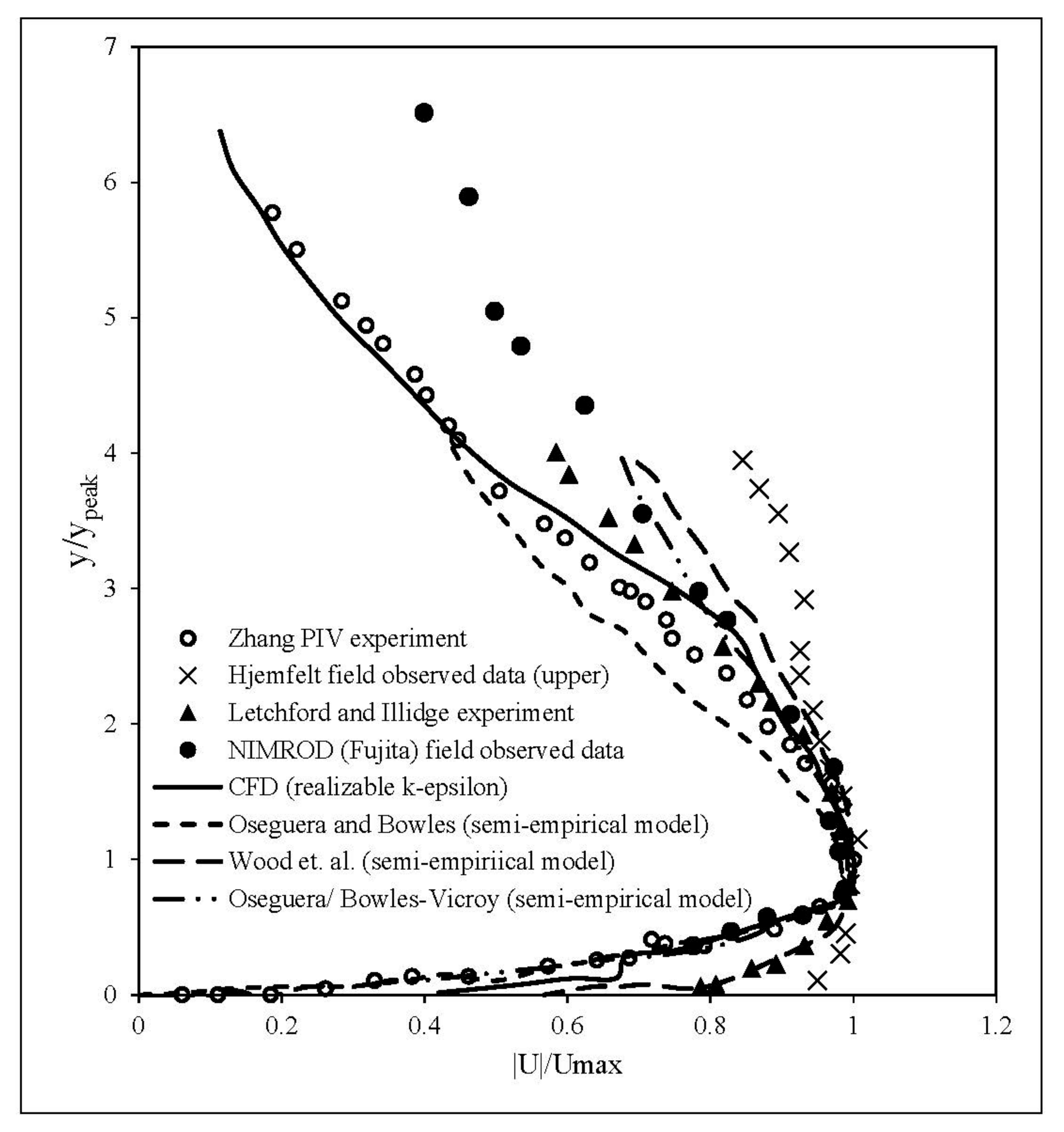
Furthermore, drawing experiences from the previous turbulent Atmospheric Boundary Layer (ABL) studies [54,55], when the flow is Re independent, the pressure force is much more significant than the skin friction force, and the pressure force would dominate the total resultant force. As the impinging jet flow in the present study becomes Re-independent from onwards, more emphasis will be placed on the pressure force from an engineering perspective. Apart from validating with the experimental data from XH, a further validation with the experimental data from ZG was performed. By validating with two experiments, it is ensured that the results of impinging jet model can be applied to a range of Re and H/D. The values were and in the experiment of ZG. The validation of the CFD results with ZG published experimental results (Figure 4) shows reasonably good agreement. The maximum deviation between our CFD and ZG is around 10%. Furthermore, the present CFD results are also compared with the results that were obtained from the steady-state analytical models for the mean speed, as proposed by Oseguera and Bowles [38], Vicroy [39], and Wood et al. [32], and the field observed data by Fujita [5] and Hjelmfelt [3]. It can be concluded that the current numerical results are within the limits of all existing prediction methods and field measurement found in the open literature. Moreover, it also confirms that the CFD results near the wall boundary constitute an accurate and physical prediction of the mean wind profile of the downburst wind shear.
3. Results and Discussion
The mean pressure field is measured in terms of the pressure coefficient ():
where , , and are taken to be mean static gauge pressure, atmospheric gauge pressure, density of air, and inlet jet velocity, respectively. The Reynolds number chosen for the study in this section is fixed at Re = 20,000.
The radial distribution of obtained from URANS and steady RANS simulation are extracted at , which is the height from the ground where the peak velocity is found at each radial location.
The values of from the RANS simulations are illustrated in Figure 5, where /D is shown for different values of and . Across all of the radial locations (from to ), /D is approximately constant for the cases of . The exact value is determined to be 0.032 for the case of .
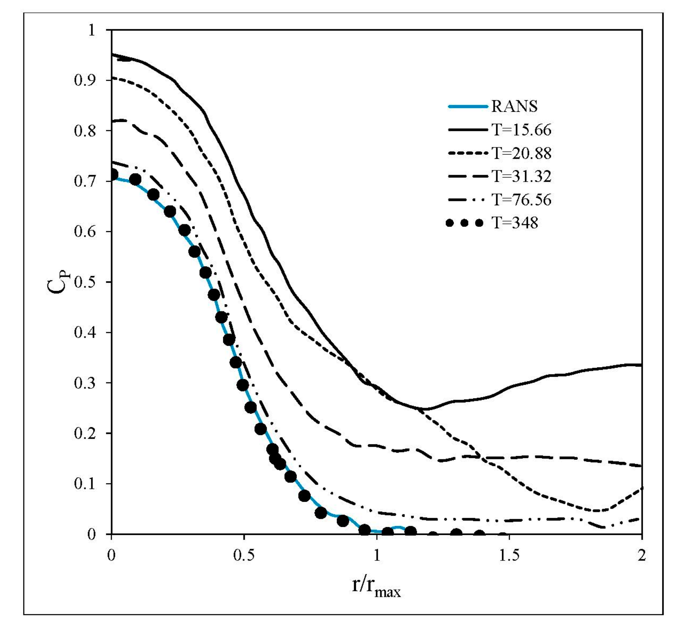
The evolution of the with time is now investigated at for the case of . The of the URANS simulation is extracted at flow-times, given in Table 2. These instances are between the release of the steady jet from the inlet to the complete convection of the primary ring vortices out of the computational domain . The first value of corresponds to the instance when the downdraft reaches the surface.
According to Fujita [1] and Mason et al. [50], the location of maximum velocity ( would also be the location of the minimum in the radial distribution of the pressure. From Figure 6, the can be deduced when is first reduced to zero from a high positive value (at ). Hence, deduced from the pressure data is determined to be one diameter (). This value of that is reported here is relatively accurate and it is close to the earlier prediction [28] of maximum velocity location of obtained from RANS simulation, and in URANS simulation. Both types of the simulations had the same , as in the present study.
The variation of in Figure 6 from URANS simulation matches the qualitative account of [1] for the pressure variation along the radial direction. As the flow-time reaches the non-dimensional value of , which is considered to be long enough after the initial touchdown of the downburst at , the value of coincides with the result from the steady RANS simulation, which has already been validated with published models and data. Therefore, at flow-time of , the impinging jet is at a quasi-steady state. The reason why there is no increase in at at T = 348 in Figure 6 for URANS simulation could be that the primary vortex rings have already convected away at that time, which was also the explanation made by Chay and Letchford [15]. A similar plot of radial distribution of was published by Chay and Letchford [15] who reported the “sharp decrease” of static pressure and restoration of the static pressure back to atmospheric pressure at maximum velocity location , as well as no “negative static pressure region” in their RANS simulation. These reported features can be observed from the present URANS simulation results, including that the is restored back to the atmospheric pressure at the maximum velocity location at . A high positive pressure at is observed in both the RANS simulation results and URANS simulation results in Figure 6. This flow feature was reported by Cui and Chen [18] when they studied the spatial distribution of across a curved-roof placed at using RANS simulation. The high positive pressure dome at stagnation region around was also found in the observed field data by Fujita [1].
4. Conclusions
The evolution of the pressure coefficient with time derived from the URANS simulation of a steady impinging jet flow has been shown to approach the RANS results after a sufficiently long time period (). The RANS results have been validated with existing field observed data [1,3,6], published experiments [21,29], and the semi-empirical velocity models [32,39]. The results have been validated with published literature to ensure that it is representative of the major feature in the dry microburst-like wind. The development of the pressure field from the initial release of the downdraft to a quasi-steady state is also consistent with the data from published field observations. Present study shows encouraging results that the methodology assures an accurate evaluation of the wind load impact, specifically for the mean pressure coefficient, which is caused by dry microburst-like wind on engineering structures and buildings. The height where the peak velocity occur for r/D = 1 to 2.5 and H/D = 2 to 4 is found to be consistently around /D = 0.03. The distribution has been compared qualitatively with the field observed data and published experimental data. The results have an impact on understanding the variation of the mean wind load effect over engineering structures and buildings during the initial landing of the dry microburst-like wind on the ground, which is a major concern to the wind engineering community.
Acknowledgments
The research described in this paper is supported by the National Research Foundation (NRF) of Singapore and Joint Industry Programme (JIP)—Energy Research Institute (ERI@N) at Nanyang Technological University, Singapore.
Author Contributions
T.S.S., M.S. and N.S. conceived the computational study; T.S.S. performed the simulations; T.S.S. and M.S. analyzed the data; N.S. contributed analysis tools; T.S.S. and M.S. wrote the paper with valuable input from N.S.
Conflicts of Interest
The authors declare no conflict of interest.
References
- Fujita, T.T. The Downburst: Microburst and Macroburst: Report of Projects NIMROD and JAWS, Satellite and Mesometeorology Research Project; Dept. of the Geophysical Sciences, University of Chicago Press: Chicago, IL, USA, 1985. [Google Scholar]
- Atkins, N.T.; Wakimoto, R.M. Wet Microburst Activity over the Southeastern United States: Implications for Forecasting. Weather Forecast. 1991, 6, 470–482. [Google Scholar] [CrossRef]
- Hjelmfelt, M.R. Structure and Life Cycle of Microburst Outflows Observed in Colorado. J. Appl. Meteorol. 1988, 27, 900–927. [Google Scholar] [CrossRef]
- Mårtensson, G.; Skote, M.; Malmqvist, M.; Falk, M.; Asp, A.; Svanvik, N.; Johansson, A.V. Rapid PCR amplification of DNA utilizing Coriolis effects. Eur. Biophys. J. 2006, 35, 453–458. [Google Scholar] [CrossRef] [PubMed]
- Fujita, T.T. Objectives, operation, and results of Project NIMROD. In Proceedings of the 11th Conference on Severe Local Storms, Kansas City, MO, USA, 2–5 October 1979; American Meteorological Society: Boston, MA, USA, 1979; pp. 259–266. [Google Scholar]
- McCarthy, J.; Wilson, J.W.; Fujita, T.T. The Joint Airport Weather Studies Project; Bulletin of the American Meteorological Society; American Meteorological Society: Boston, MA, USA, 1982; Volume 63, p. 15. [Google Scholar]
- Wolfson, M.M.; DiStafano, J.T.; Forman, B.E. The FLOWS (FAA-Lincoln Laboratory Operational Weather Studies) Automatic Weather Station Network in Operation; Defense Technical Information Center: Fort Belvoir, VA, USA, 1987. [Google Scholar]
- Choi, E.C.C. Field measurement and experimental study of wind speed profile during thunderstorms. J. Wind Eng. Ind. Aerodyn. 2004, 92, 275–290. [Google Scholar] [CrossRef]
- Burlando, M.; Romanić, D.; Solari, G.; Hangan, H.; Zhang, S. Field data analysis and weather scenario of a downburst event in Livorno, Italy, on 1 October 2012. Mon. Weather Rev. 2017, 145, 3507–3527. [Google Scholar] [CrossRef]
- De Gaetano, P.; Repetto, M.P.; Repetto, T.; Solari, G. Separation and classification of extreme wind events from anemometric records. J. Wind Eng. Ind. Aerodyn. 2014, 126, 132–143. [Google Scholar] [CrossRef]
- Solari, G.; Repetto, M.P.; Burlando, M.; De Gaetano, P.; Pizzo, M.; Tizzi, M.; Parodi, M. The wind forecast for safety management of port areas. J. Wind Eng. Ind. Aerodyn. 2012, 104–106, 266–277. [Google Scholar] [CrossRef]
- Gunter, W.S.; Schroeder, J.L. High-resolution full-scale measurements of thunderstorm outflow winds. J. Wind Eng. Ind. Aerodyn. 2015, 138, 13–26. [Google Scholar] [CrossRef]
- Holmes, J.D.; Hangan, H.M.; Schroeder, J.L.; Letchford, C.W.; Orwig, K.D. A forensic study of the Lubbock-Reese downdraft of 2002. Wind Struct. 2008, 11, 137–152. [Google Scholar] [CrossRef]
- Holmes, J.D. Modelling of extreme thunderstorm winds for wind loading of structures and risk assessment. In Proceedings of the Tenth International Conference on Wind Engineering, Copenhagen, Denmark, 21–24 June 1999; Volume 2, pp. 1409–1416. [Google Scholar]
- Chay, M.T.; Letchford, C.W. Pressure distributions on a cube in a simulated thunderstorm downburst—Part A: Stationary downburst observations. J. Wind Eng. Ind. Aerodyn. 2002, 90, 711–732. [Google Scholar] [CrossRef]
- Letchford, C.W.; Chay, M.T. Pressure distributions on a cube in a simulated thunderstorm downburst. Part B: Moving downburst observations. J. Wind Eng. Ind. Aerodyn. 2002, 90, 733–753. [Google Scholar] [CrossRef]
- Kim, J.; Hangan, H.; Ho, T.C.E. Downburst versus boundary layer induced wind loads for tall buildings. Wind Struct. 2007, 10, 481–494. [Google Scholar] [CrossRef]
- Cui, B.; Chen, Y. CFD Simulation of Curved-roof subjected to Thunderstorm Downburst. In Key Engineering Materials; Trans Tech Publications: Zürich, Switzerland, 2017; Volume 474, pp. 1243–1248. [Google Scholar]
- Nguyen, H.H.; Manuel, L.; Veers, P.S. Wind turbine loads during simulated thunderstorm microbursts. J. Renew. Sustain. Energy 2011, 3, 053104–053119. [Google Scholar] [CrossRef]
- Nguyen, H.H.; Manuel, L. Thunderstorm downburst risks to wind farms. J. Renew. Sustain. Energy 2013, 5, 013120. [Google Scholar] [CrossRef]
- Zhang, Y. Study of Microburst-Like Wind and Its Loading Effects on Structures Using Impinging Jet and Cooling Source Approach; Iowa State University: Ames, IA, USA, 2013. [Google Scholar]
- Zhang, Y.; Hu, H.; Sarkar, P.P. Modeling of microburst outflows using impinging jet and cooling source approaches and their comparison. Eng. Struct. 2013, 56, 779–793. [Google Scholar] [CrossRef]
- Anderson, J.R.; Orf, L.G.; Straka, J.M. A 3-D model system for simulating thunderstorm microburst outflows. Meteorl. Atmos. Phys. 1992, 49, 125–131. [Google Scholar] [CrossRef]
- Orf, L.G.; Anderson, J.R.; Straka, J.M. A Three-Dimensional Numerical Analysis of Colliding Microburst Outflow Dynamics. J. Atmos. Sci. 1996, 53, 2490–2511. [Google Scholar] [CrossRef]
- Orf, L.G.; Anderson, J.R. A Numerical Study of Traveling Microbursts. Mon. Weather Rev. 1999, 127, 1244–1258. [Google Scholar] [CrossRef]
- Orf, L.G.; Kantor, E.; Savory, E. Simulation of a downburst-producing thunderstorm using a very high-resolution three-dimensional cloud model. J. Wind Eng. Ind. Aerodyn. 2012, 104–106, 547–557. [Google Scholar] [CrossRef]
- Vermeire, B.C.; Orf, L.G.; Savory, E. A parametric study of downburst line near-surface outflows. J. Wind Eng. Ind. Aerodyn. 2011, 99, 226–238. [Google Scholar] [CrossRef]
- Kim, J.; Hangan, H. Numerical simulations of impinging jets with application to downbursts. J. Wind Eng. Ind. Aerodyn. 2007, 95, 279–298. [Google Scholar] [CrossRef]
- Xu, Z.; Hangan, H. Scale, boundary and inlet condition effects on impinging jets. J. Wind Eng. Ind. Aerodyn. 2008, 96, 2383–2402. [Google Scholar] [CrossRef]
- Chay, M.T.; Albermani, F.; Wilson, R. Numerical and analytical simulation of downburst wind loads. Eng. Struct. 2006, 28, 240–254. [Google Scholar] [CrossRef] [Green Version]
- Li, C.; Li, Q.S.; Xiao, Y.Q.; Ou, J.P. Simulations of moving downbursts using CFD. In Proceedings of the Seventh Asia-Pacific Conference on Wind Engineering, Taiwan, 8–12 November 2009. [Google Scholar]
- Wood, G.S.; Kwok, K.C.S.; Motteram, N.A.; Fletcher, D.F. Physical and numerical modelling of thunderstorm downbursts. J. Wind Eng. Ind. Aerodyn. 2001, 89, 535–552. [Google Scholar] [CrossRef]
- Sengupta, A.; Sarkar, P.P. Experimental measurement and numerical simulation of an impinging jet with application to thunderstorm microburst winds. J. Wind Eng. Ind. Aerodyn. 2008, 96, 345–365. [Google Scholar] [CrossRef]
- Das, K.K.; Ghosh, A.K.; Sinhamahapatra, K.P. Experimental and Numerical simulation of the Translational Downburst using impinging jet model. Int. J. Eng. Sci. Technol. (IJEST) 2011, 3, 4656–4667. [Google Scholar]
- Landreth, C.C.; Adrian, R.J. Impingement of a low Reynolds number turbulent circular jet onto a flat plate at normal incidence. Exp. Fluids 1990, 9, 74–84. [Google Scholar] [CrossRef]
- Zhang, Y.; Hu, H.; Sarkar, P.P. Comparison of microburst-wind loads on low-rise structures of various geometric shapes. J. Wind Eng. Ind. Aerodyn. 2014, 133, 181–190. [Google Scholar] [CrossRef]
- Zhang, Y.; Sarkar, P.; Hu, H. An experimental study on wind loads acting on a high-rise building model induced by microburst-like winds. J. Fluids Struct. 2014, 50, 547–564. [Google Scholar] [CrossRef]
- Oseguera, R.M.; Bowles, R.L. A Simple, Analytic 3-Dimensional Downburst Model Based on Boundary Layer Stagnation Flow; National Aeronautics and Space Administration, Langley Research Center: Hampton, VA, USA, 1988. [Google Scholar]
- Vicroy, D.D. A Simple, Analytical, Axisymmetric Microburst Model for Downdraft Estimation; National Aeronautics and Space Administration, Langley Research Center: Hampton, VA, USA, 1991. [Google Scholar]
- Li, C.; Li, Q.S.; Xiao, Y.Q.; Ou, J.P. A revised empirical model and CFD simulations for 3D axisymmetric steady-state flows of downbursts and impinging jets. J. Wind Eng. Ind. Aerodyn. 2012, 102, 48–60. [Google Scholar] [CrossRef]
- ANSYS Fluent User Manual by ANSYS Inc. Available online: www.ansys.com (accessed on 5 January 2018).
- Holmes, J.D. Wind turbines-Part 1: Design Requirements. In Wind Loading of Structures; IEC 61400-1; Taylor & Francis International Electrotechnical Commission: Boca Raton, FL, USA, 2007. [Google Scholar]
- Fujita, T.T. Tornadoes and Downbursts in the Context of Generalized Planetary Scales. J. Atmos. Sci. 1981, 38, 1511–1534. [Google Scholar] [CrossRef]
- Skote, M. Scaling of the velocity profile in strongly drag reduced turbulent flows over an oscillating wall. Int. J. Heat Fluid Flow 2014, 50, 352–358. [Google Scholar] [CrossRef]
- Wolfstein, M. The Velocity and Temperature Distribution of One-Dimensional Flow with Turbulence Augmentation and Pressure Gradient. Int. J. Heat Mass Transf. 1969, 12, 301–318. [Google Scholar] [CrossRef]
- Shih, T.H.; Liou, W.; Shabbir, Z.Y.; Zhu, J. A New k-ε Eddy Viscosity Model for High Reynolds Number Turbulent Flows—Model Development and Validation. Comput. Fluids 1995, 24, 227–238. [Google Scholar] [CrossRef]
- Kader, B. Temperature and Concentration Profiles in Fully Turbulent Boundary Layers. Int. J. Heat Mass Transf. 1981, 24, 1541–1544. [Google Scholar] [CrossRef]
- Leonard, B.P. A stable and accurate convective modelling procedure based on quadratic upstream interpolation. Comput. Methods Appl. Mech. Eng. 1979, 19, 59–98. [Google Scholar] [CrossRef]
- Versteeg, H.K.; Malalasekera, W. An Introduction to Computational Fluid Dynamics: The Finite Volume Method; Pearson Education Limited: London, UK, 2007. [Google Scholar]
- Mangani, L.; Bianchini, C. Heat transfer applications in turbomachinery. In Proceedings of the OpenFOAM International Conference, London, UK, 26–27 November 2007. [Google Scholar]
- Mason, M.S.; Letchford, C.W.; James, D.L. Pulsed wall jet simulation of a stationary thunderstorm downburst, Part A: Physical structure and flow field characterization. J. Wind Eng. Ind. Aerodyn. 2005, 93, 557–580. [Google Scholar] [CrossRef]
- Das, K.K.; Ghosh, A.K.; Sinhamahapatra, K.P. Development of a numerical code for simulation of dry microburst using impinging jet model. Int. J. Appl. Math. Mech. 2011, 7, 56–71. [Google Scholar]
- Lim, H.C.; Castro, I.P.; Hoxey, R.P. Bluff bodies in deep turbulent boundary layers: Reynolds-number issues. J. Fluid Mech. 2007, 571, 97–118. [Google Scholar] [CrossRef]
- Claus, J.; Coceal, O.; Thomas, T.G.; Branford, S.; Belcher, S.E.; Castro, I. Wind-Direction Effects on Urban-Type Flows. Bound. Layer Meteorol. 2012, 142, 265–287. [Google Scholar] [CrossRef]
- Claus, J.; Krogstad, P.Å.; Castro, I. Some Measurements of Surface Drag in Urban-Type Boundary Layers at Various Wind Angles. Bound. Layer Meteorol. 2002, 145, 407–442. [Google Scholar] [CrossRef]
Figure 1.
Two-dimensional (2D) axisymmetric computational domain.

Figure 2.
Normalised radial velocity |Urad|/Ujet at r/D = 1 (grid convergence).

Figure 3.
Comparison of Computational Fluid Dynamics (CFD) results (RANS with the realizable k-ε turbulence model) using mesh M4 with Xu and Hangan [29] experimental (EXP) data (Re = 20,000) at radial locations r/D = 1, 1.4, 2.0 and 2.5.
Figure 3.
Comparison of Computational Fluid Dynamics (CFD) results (RANS with the realizable k-ε turbulence model) using mesh M4 with Xu and Hangan [29] experimental (EXP) data (Re = 20,000) at radial locations r/D = 1, 1.4, 2.0 and 2.5.

Figure 4.
CFD results (RANS) validated with published particle image velocimetry (PIV) experimental data of Zhang. [21] The present result using the realizable k-ε turbulence model at Re = 288,046, H/D = 2 at r/D = 1.0 is shown as the solid line. Umax is the maximum speed of the outflow near the ground, and ypeak is the corresponding height where the maximum speed occurs.

Figure 5.
Effects of H/D on the normalized position where the peak velocity is found. From RANS at Re = 20,000.
Figure 5.
Effects of H/D on the normalized position where the peak velocity is found. From RANS at Re = 20,000.
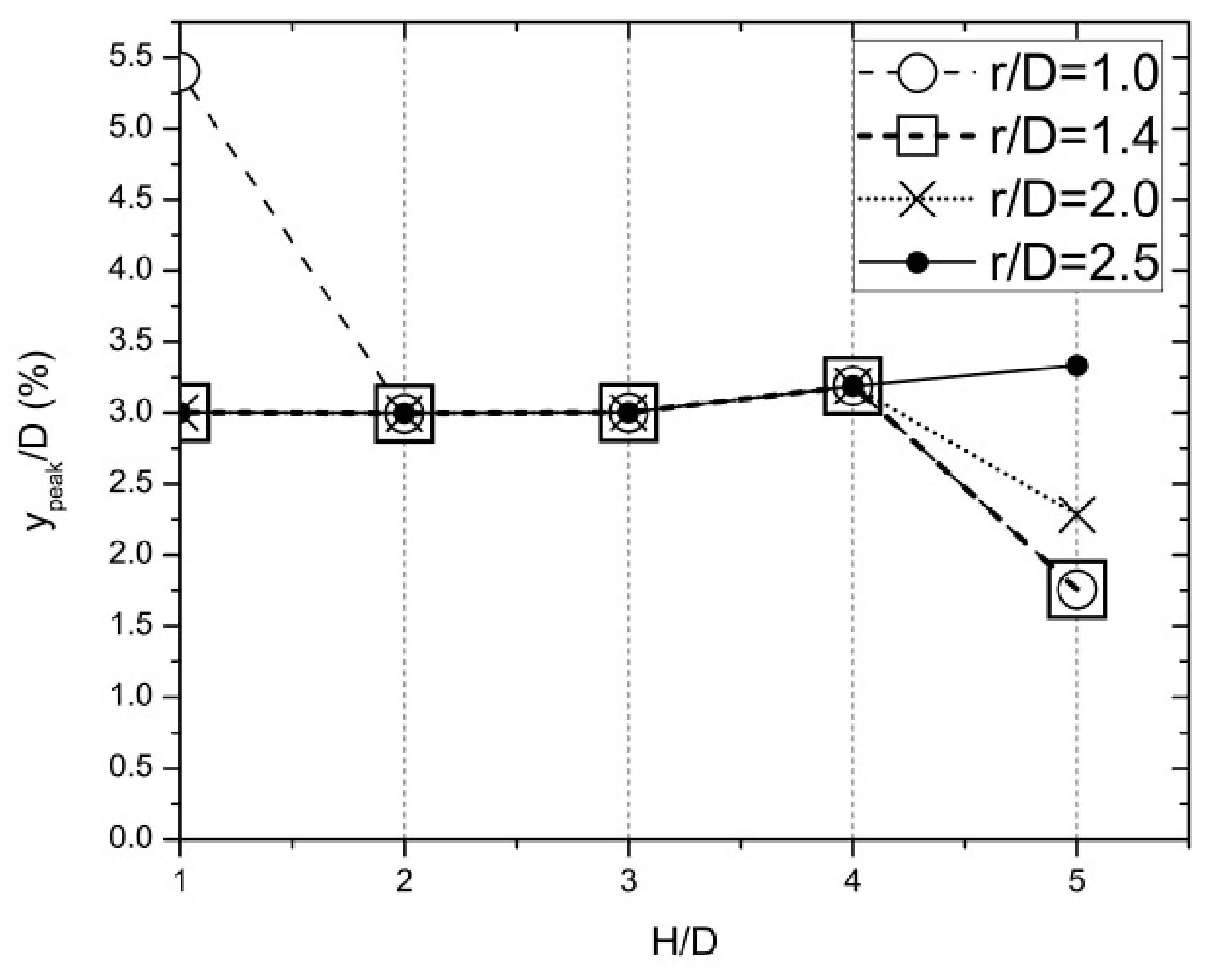
Figure 6.
Radial distribution of the mean pressure coefficient obtained from present steady and transient simulations. Radial distribution of the mean pressure coefficient obtained from the steady and transient simulations. The pressure is taken from for the case of at .
Figure 6.
Radial distribution of the mean pressure coefficient obtained from present steady and transient simulations. Radial distribution of the mean pressure coefficient obtained from the steady and transient simulations. The pressure is taken from for the case of at .


Table 1.
Mesh sizes for the purpose of grid convergence.
| Mesh Case Notations | M1 | M2 | M3 | M4 |
| Number of Elements | 565,566 | 66,861 | 38,412 | 25,144 |
Table 2.
Flow time monitored. is the dimensional time in seconds (s). is the non-dimensionalised time.
Table 2.
Flow time monitored. is the dimensional time in seconds (s). is the non-dimensionalised time.
| t (s) | 0.045 | 0.060 | 0.090 | 0.220 | 1.00 |
| 15.7 | 20.9 | 31.3 | 76.6 | 348 |
© 2018 by the authors. Licensee MDPI, Basel, Switzerland. This article is an open access article distributed under the terms and conditions of the Creative Commons Attribution (CC BY) license (http://creativecommons.org/licenses/by/4.0/).
Share and Cite
MDPI and ACS Style
Skote, M.; Sim, T.S.; Srikanth, N. Temporal Variation of the Pressure from a Steady Impinging Jet Model of Dry Microburst-Like Wind Using URANS. Computation 2018, 6, 2. https://doi.org/10.3390/computation6010002
AMA Style
Skote M, Sim TS, Srikanth N. Temporal Variation of the Pressure from a Steady Impinging Jet Model of Dry Microburst-Like Wind Using URANS. Computation. 2018; 6(1):2. https://doi.org/10.3390/computation6010002
Chicago/Turabian StyleSkote, Martin, Tze Siang Sim, and Narasimalu Srikanth. 2018. "Temporal Variation of the Pressure from a Steady Impinging Jet Model of Dry Microburst-Like Wind Using URANS" Computation 6, no. 1: 2. https://doi.org/10.3390/computation6010002
Note that from the first issue of 2016, this journal uses article numbers instead of page numbers. See further details here.