Modeling Confined Cell Migration Mediated by Cytoskeleton Dynamics

Abstract

Cell migration is an important biological process that has generated increasing interest during the last several years. This process is based on three phases: protrusion at the front end of the cell, de-adhesion at the rear end and contraction of the cell body, all of them coordinated due to the polymerization/depolymerization of certain cytoskeletal proteins. The aim of this work is to present a mathematical model to simulate the actin polymerization/depolymerization process that regulates the final outcome of cell migration process, considering all the above phases, in a particular case: when the cell is confined in a microfluidic channel. Under these specific conditions, cell migration can be approximated by using one-dimensional simulations. We will propose a system of reaction–diffusion equations to simulate the behavior of the cytoskeletal proteins responsible for protrusion and contraction in the cell, coupled with the mechanical response of the cell, computing its deformations and stresses. Furthermore, a numerical procedure is presented in order to simulate the whole process in a moving and deformable domain corresponding to the cell body.

1. Introduction

Actin polymerization in cells is an essential process in a wide range of biological phenomena. The coordinate polymerization of these proteins controls the correct movement of the cell, regulating its rigidity, activating its migration or taking part in the mitosis process. In cell migration, the actin–myosin interaction and the actin polymerization itself generates mechanisms that favor the cell advance: a migrating cell creates a protrusion in the migration direction by actin polymerization at the leading edge; then, the cell adheres the leading edge to the surface and de-adheres at the rear; finally, the whole cell contracts due to forces generated by the actin–myosin network and it moves forward. A detailed description can be found in [1,2]. Cell migration is crucial in the development of biological processes such as chemotaxis, cancer metastasis or tissue regeneration. Understanding how the mechanical factors are able to regulate cell movement offers the possibility of developing new therapies to, for example, control the advance of invasive tumor cells. In vitro works allow for considering cell migration as a process regulated mainly by the actin filaments’ polymerization inside the cell (see [3]). As mentioned before, cell migration can be simplified assuming a mechanical cycle of three main phases: protrusion due to actin polymerization, adhesion and contraction due to the actin–myosin interaction. Increasing the knowledge of the actin polymerization process in combination with the contractile capacity of the actin–myosin interactions is crucial to understanding the role of mechanical conditions on the cell migration process (see [4,5]).

Cell migration is the aim of a significant number of works, such as in silico and in vitro perspectives. Several mathematical models were proposed in order to simulate this process, but each of them focused on different mechanisms such as protrusion, adhesion or contraction. Complete reviews of these different models can be found in [6] and more recently in [7]. For example, Refs. [4,5,8] considered one-dimensional mathematical models to compute the deformation and stress undergone by the cell, considering a viscoelastic behavior, together with the actin and myosin concentrations. George et al. [9] also presented a two-dimensional model to describe cell deformation and movement, coupling its behavior with biochemical processes. Moreover, the relationship between the cell velocity and traction forces due to the involved phenomena (protrusion, contraction and adhesion) were studied in [10,11,12] for the two-dimensional case. Another approach presented in [13,14] considered the cell as a two-phase continuum material, where one of the phases is the cytosol and the other the viscous, actin network capable of contracting and swelling. Finally, in [15], a three-dimensional finite element model to simulate the cell migration on a surface was studied, focusing on the mechanical aspect of the process.

Moreover, regarding in vitro experiments, during the last several years, researchers have focused their interest on three-dimensional cell migration and on the usage of microfluidic devices to determine the mechanical properties of cells. In these types of devices, cells are confined to the walls, and the migration mechanisms are different from the two-dimensional case. For example, Wilson et al. [2] studied leading edge protrusion during chemotactic migration by microfluidic channels. There, they focused on the actin structures driving protrusion in three-dimensional environments, identifying two distinct actin networks, and they proposed the mechanical interaction between them as begin the responsible for forward protrusion. Moreover, Mak et al. [16] presented a microfluidic device to study the cell migration in response to physical spatial gradients. Regarding the models adapted to these types of devices, Hawkins et al. [17] presented a mechanism of cell motility coupling actin polymerization to geometric confinement. Later, in [18], they completed the previous one-dimensional model including the effect of the contractile activity of the myosin motors. Finally, Aubry et al. [19] presented a two-dimensional mechanical model to simulate the cell migration through a micro-channel in order to describe the mechanical behavior of both the cytoplasm and the nucleus. The importance of studying cell migration in confined micro-environments was stated by Stroka et al. [20], gathering different assays developed to provide information about the mechanisms of cell migration.

As a first approach and in order to obtain a simple model to predict the direction and magnitude of cell migration, we focus our interest on the interstitial migration, that is, the cell movement through microfluidic channels. Due to the complexity of the whole cell migration process when considering a three-dimensional scenario, we propose simplifying the process solving a suitable one-dimensional model. This approach is appropriate when considering interstitial migration in microfluidic devices due to the significant differences between the spatial dimensions in the channels. Therefore, the aim of this work is to obtain a one-dimensional mathematical model to simulate the behavior of the main components regulating cytoskeleton (CSK) dynamics in order to predict the cell migration, the actin and myosin spatio-temporal distribution and the deformations and stresses undergone by the cells.

With this aim in mind, and based on the previous works of Gracheva and Othmer [8] and Larripa and Mogilner [4], we will propose a system of coupled reaction–diffusion equations to model the actin polymerization process together with the myosin contractile effect on the cell. Moreover, actin and myosin concentrations are a key factor in the cell migration process since they directly affect the mechanical deformability/contractility of the cell. In addition, we will couple the previous equations with the mechanical response of the cell, computing its deformation and stress. The cell body is viewed as an elastic material, including the contraction and protrusion effects due to myosin and actin concentrations. The main differences of the model proposed here from those mentioned in the bibliography [4,5,8] are considering and computing not only the bound actin and bound myosin concentrations but also the free actin and free myosin densities. Reaction–diffusion equations including effects such as polymerization, depolymerization and positive feedbacks are used to model the dynamical behavior of the actin and myosin densities. Moreover, the proposed model includes also the cell growth domain during the process and the adhesion and de-adhesion phenomenon with the substrate. In order to carry out the numerical simulations of the proposed model, we will use a suitable spatial-temporal integration scheme that allows us to compute the effect of the actin and myosin densities on the cytoskeleton deformation.

The model presented here is a first and simple approach of the interstitial migration process. The final aim is to implement a simple procedure to model the behavior of a cell in a microfluidic channel, mainly in the bifurcations, in order to obtain a quick tool to predict the cell behavior in these types of devices in the laboratory.

This work is organized as follows. In Section 2, we will describe the mathematical model to simulate the migration process. Moreover, Section 2.2 is devoted to the proposed numerical procedure to compute the deformations and stresses of a cell during interstitial migration. In Section 3, we will present the numerical results obtained in the simulation of the considered cell migration process. Finally, Section 3 collects some conclusions and comments about future work.

2. Materials and Methods

In this section, we present the mathematical model and the different mechanisms considered to simulate the cell migration process. Moreover, we briefly describe the numerical method used to solve the proposed model.

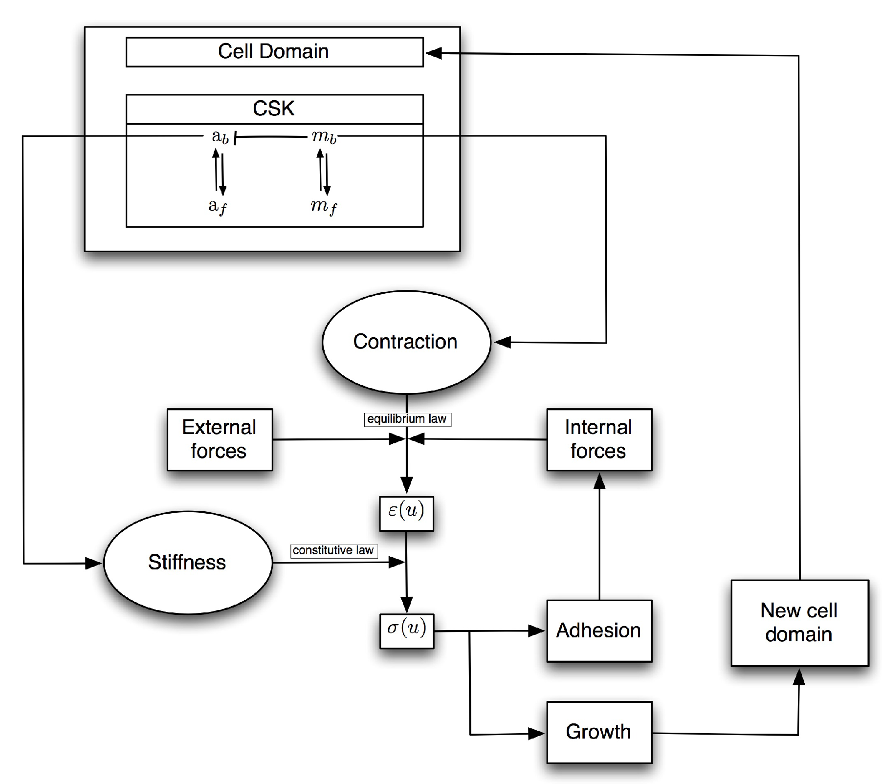
2.1. Mathematical Model

We assume that the cell movement is regulated by the CSK dynamics, the actin and myosin concentrations and the deformations and stresses undergone by the cell.

Figure 1 shows a scheme of the different interactions considered in the model: the evolution of the actin and myosin concentrations is governed by means of reaction–diffusion equations; the cellular deformations and stresses are related by means of an elastic constitutive law, where the cell stiffness depends on the actin concentration; the force contraction generated by the cell is due to the myosin bound to the actin; the cell growth during the process is due to the stress generated at the ends of the cell body; and the adhesion/failure is also regulated by the existent stress at the ends, increasing/decreasing the friction with the substrate.

Let ${\Omega }_0=(0,L_0)$ be the initial one-dimensional domain corresponding to the cell geometry with $L_0$ the cell length (see Figure 2). We assume that the cell occupies the region $\left(r\right(t),f(t\left)\right)$ at each time instant t, where $r\left(t\right)$ and $f\left(t\right)$ denote the rear and front ends, respectively; thus, $r\left(0\right)=0,f\left(0\right)=L_0$ and $\Omega \left(t\right)=\left(r\right(t),f(t\left)\right)$.

The problem we aim to solve is to compute the displacement $u=u(x,t)$ and the stress $\sigma =\sigma (x,t)$, suffered by the cell body $\Omega \left(t\right)$ during the time interval of interest $(0,T)$. Note that u and $\sigma$ are scalar variables since we focus on the one-dimensional problem. In order to compute these unknowns, the actin $(a_b,a_f)$ and myosin $(m_b,m_f)$ concentrations are also considered, distinguishing between the active and inactive (bound and free) behaviors.

2.1.1. Mechanical Equilibrium

The quasi-static equilibrium of the cell is governed by the mechanical equilibrium equation

$${\displaystyle \frac{\partial \sigma }{\partial x}}(x,t)+g=0\mathrm{in}\Omega \left(t\right)\times (0,T),$$

where g denotes the internal volume forces acting on the cell body. We assume that these volume forces are only due to the adhesion of the cell with the substrate, that is, $g=g(x,t)=\beta v(x,t)$, and

$${\displaystyle \frac{\partial \sigma }{\partial x}}(x,t)=\beta v(x,t)=\beta {\displaystyle \frac{\partial u}{\partial t}}(x,t)\mathrm{in}\Omega \left(t\right)\times (0,T),$$

(1)

where $v(x,t)$ denotes the velocity of the cell body and $\beta$ is the friction coefficient, which measures the strength of adhesion between the cell and the substrate. The larger this coefficient is, the larger the friction that is produced.

2.1.2. Constitutive Law

We consider that the cell is an elastic material; therefore, following [8], we can relate the stress with the resulting deformation through an elastic passive stress and a contractile active stress:

$$\sigma (x,t)={\sigma }_{el}(x,t)+\tau (x,t)=E(x,t){\displaystyle \frac{\partial u}{\partial x}}(x,t)+\tau (x,t).$$

The contractile stress is due to the myosin proteins bound to the actin filaments in the cytoskeleton of the cell; therefore, we assume that

$$\tau (x,t)={\eta }_m{m}_b(x,t),$$

where $m_b$ denotes the concentration of bound myosin proteins and ${\eta }_m$ is a characteristic myosin stress parameter. The elastic passive stress is described through a proportionality relation between this stress and the cell strain. The elastic modulus $E(x,t)$ is considered depending on the position and time since the mechanical properties of the cell change also with position and time, with a dependence on the actin density. Due to this, the elastic modulus $E(x,t)$ depends on the number of bound actin monomers in the cytoskeleton, that is,

$$E(x,t)=E_0{a}_b(x,t),$$

where $E_0$ is a constant value.

Summing up, the mechanical behavior law remains:

$$\sigma (x,t)=E_0{a}_b(x,t){\displaystyle \frac{\partial u}{\partial x}}(x,t)+{\eta }_m{m}_b(x,t).$$

(2)

Gathering Equations (1) and (2), the proposed differential equation to solve the displacement of a cell is the following:

$$\beta {\displaystyle \frac{\partial u}{\partial t}}(x,t)-{\displaystyle \frac{\partial }{\partial x}}\left(E_0{a}_b(x,t){\displaystyle \frac{\partial u}{\partial x}}(x,t)\right)={\eta }_m{\displaystyle \frac{\partial m_b}{\partial x}}(x,t)\mathrm{in}\Omega \left(t\right)\times (0,T).$$

(3)

2.1.3. Reaction–Diffusion Equations

The myosin behavior is described by two variables: the active and inactive myosin $(m_b,m_f)$. The active myosin concentration corresponds to the density of myosin proteins bound to the actin filaments and the inactive myosin concentration is due to the free myosin proteins. Analogously, the actin behavior is divided into the active and inactive concentrations $(a_b,a_f)$. The active concentration corresponds to the bound actin monomers conforming the filaments found in the cytoskeleton, and the inactive concentration is the free actin monomers flowing in the cell. In order to compute their concentrations, we propose the following reaction–diffusion equations that describe the behavior of the different densities including the diffusion and advection terms:

$$\begin{array}{c}{\displaystyle \frac{\partial a_b}{\partial t}}=D_{ab}\frac{{\partial }^2{a}_b}{\partial x^2}-\frac{\partial }{\partial x}\left(a_{b}v\right)+F_a(a_b,a_f,m_b),\hfill \end{array}$$

(4)

$$\begin{array}{c}{\displaystyle \frac{\partial a_f}{\partial t}}=D_{af}\frac{{\partial }^2{a}_f}{\partial x^2}-\frac{\partial }{\partial x}\left(a_{f}v\right)-F_a(a_b,a_f,m_b),\hfill \end{array}$$

(5)

$$\begin{array}{c}{\displaystyle \frac{\partial m_b}{\partial t}}=D_{mb}\frac{{\partial }^2{m}_b}{\partial x^2}-\frac{\partial }{\partial x}\left(m_{b}v\right)+F_m\left(m_f\right),\hfill \end{array}$$

(6)

$$\begin{array}{c}{\displaystyle \frac{\partial m_f}{\partial t}}=D_{mf}\frac{{\partial }^2{m}_f}{\partial x^2}-\frac{\partial }{\partial x}\left(m_{f}v\right)-F_m\left(m_f\right).\hfill \end{array}$$

(7)

Here, $D_{ab}$, $D_{af}$, $D_{mb}$ and $D_{mf}$ are diffusion coefficients and $F_a$ and $F_m$ are reaction functions that define the behavior of the specific concentrations. The advection terms in the equations model the transport of the different species in the cell. In this work, we consider the following reaction functions:

$$\begin{array}{c}{F}_a(a_b,a_f,m_b)=k_a{\displaystyle \frac{a_f}{m_b}}+\gamma {\displaystyle \frac{a_b^2}{K^2+a_b^2}}{\displaystyle \frac{a_f}{m_b}}-\delta a_b,\hfill \end{array}$$

(8)

$$\begin{array}{c}{F}_m(m_b,m_f)=k_{mp}{m}_f-k_{mdp}{m}_b.\hfill \end{array}$$

(9)

The reaction functions $F_a$ and $F_m$ are chosen in order to reproduce the behavior of actin monomers and myosin molecules in the cell cytoskeleton (see, for example, [21]). In these reaction terms, the bound actin $a_b$ plays the role of an active protein, whereas the free actin $a_f$ acts as an inactive protein. Moreover, with these forces, free actin $a_f$ is an activator of bound actin $a_b$, bound myosin $m_b$ is an inhibitor of bound actin $a_b$ and free myosin $m_f$ is an activator of bound myosin $m_b$. In Equation (8), $k_a$ and $\delta$ are the rates of activation and inactivation of actin, respectively, $\gamma$ is the rate of maximal feedback strength and K is its saturation parameter, whereas, in Equation (9) $k_{mp}$ and $k_{mdp}$ are the activation rate and the depolymerization rate of myosin molecules, respectively.

Finally, we need to complete our mathematical model with adequate boundary conditions. We assume conditions of null flux for actin and myosin concentrations (either free or bound), that is:

$$\begin{array}{c}{\displaystyle \frac{\partial a_b}{\partial x}}(r\left(t\right),t)=0,{\displaystyle \frac{\partial a_b}{\partial x}}(f\left(t\right),t)=0,\hfill \end{array}$$

(10)

$$\begin{array}{c}{\displaystyle \frac{\partial a_f}{\partial x}}(r\left(t\right),t)=0,{\displaystyle \frac{\partial a_f}{\partial x}}(f\left(t\right),t)=0,\hfill \end{array}$$

(11)

$$\begin{array}{c}{\displaystyle \frac{\partial m_b}{\partial x}}(r\left(t\right),t)=0,{\displaystyle \frac{\partial m_b}{\partial x}}(f\left(t\right),t)=0,\hfill \end{array}$$

(12)

$$\begin{array}{c}{\displaystyle \frac{\partial m_f}{\partial x}}(r\left(t\right),t)=0,{\displaystyle \frac{\partial m_f}{\partial x}}(f\left(t\right),t)=0.\hfill \end{array}$$

(13)

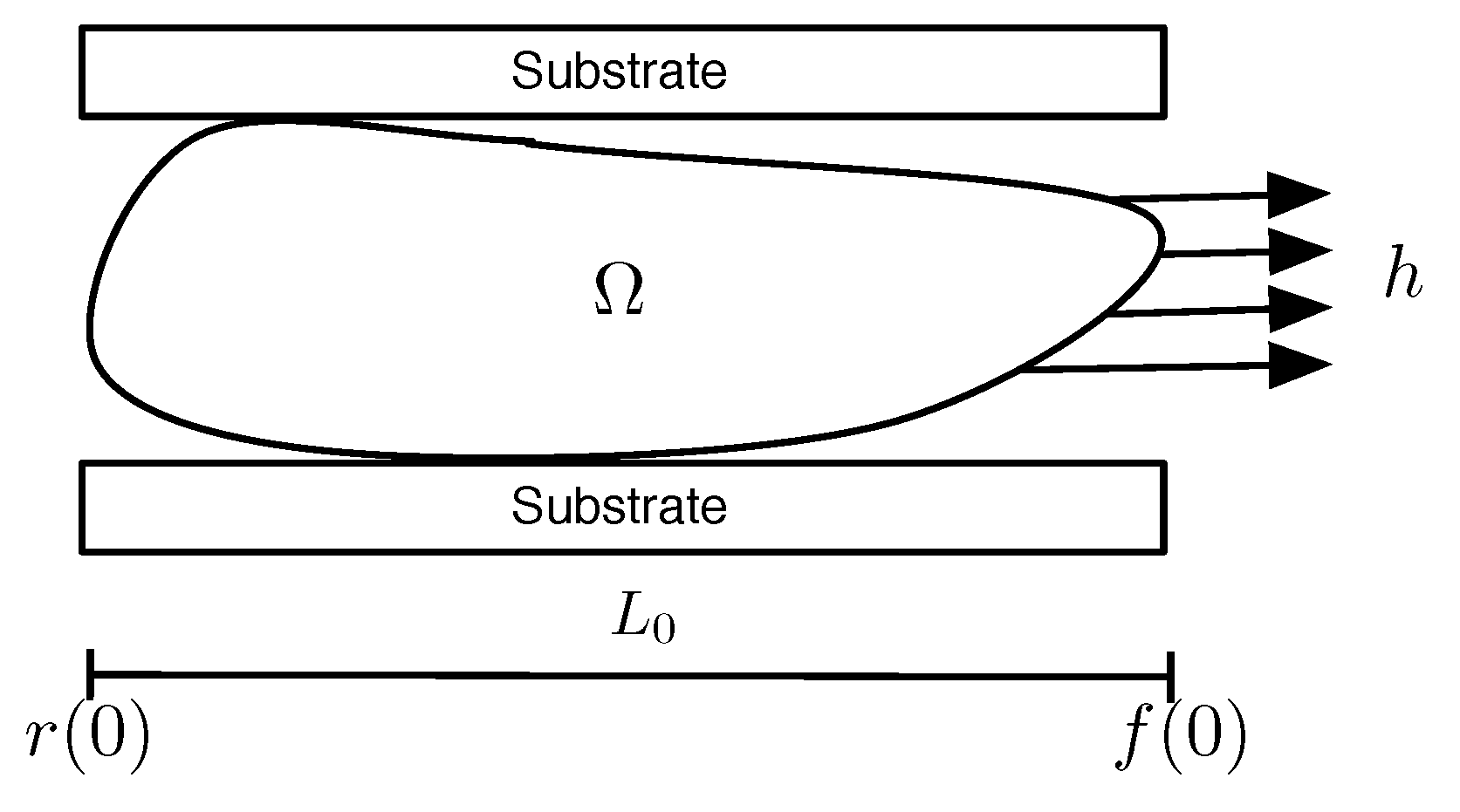
2.1.4. External Forces

In order to model the cell movement through microfluidic channels, we consider that the cell body is free of forces in the rear end ($r\left(t\right)$) and a surface force is temporarily applied to the cell membrane in the front end ($f\left(t\right)$) during a determined time interval $[t_a,t_d]$. We assume that this load is similar to that produced during an aspiration experiment. The expression for this boundary condition is the following:

$$\sigma \left(r\right(t),t)=0,\sigma \left(f\right(t),t)=h\left(t\right),$$

(14)

where h is given by:

$$h\left(t\right)=\left\{\begin{array}{cc}0,\hfill & \mathrm{if}t<t_a,\hfill \\ h_a\left(t\right),\hfill & \mathrm{if}{t}_a\le t\le t_d,\hfill \\ 0,\hfill & \mathrm{if}{t}_d<t\hfill \end{array}\right.,$$

(15)

being $h_a\left(t\right)$ a linear pressure function such that $h_a\left(t_a\right)={\sigma }_a$ and $h_a\left(t_d\right)={\sigma }_d$, with ${\sigma }_a$ and ${\sigma }_d$ the activation and deactivation pressure values and $t_a$ and $t_d$ the activation and deactivation time steps.

2.1.5. Cell Domain Growth

When external stress is applied, a growth in the cell length could happen. The model presented here assumes that this growth occurs only if the cell is mechanically deformed up to a suitable stress threshold, denoted by ${\sigma }_g$, that is:

$$\sigma (f\left(t\right),t)=h\left(t\right)\Rightarrow \begin{array}{c}\sigma (f\left(t\right),t)<{\sigma }_g\Rightarrow “\text{stable domain}”\hfill \\ \sigma (f\left(t\right),t)>{\sigma }_g\Rightarrow “\text{space to expand}”.\hfill \end{array}$$

In the second case, the cell membrane detaches from the actin cortex, creating a new space where the actin filaments in the cytoskeleton can expand and, therefore, the cell domain grows (see Figure 3). This new space is determined by using the one-dimensional relationship between strain and stress in an elastic material.

To describe the behavior of the different species in the cell when this new space is generated (that is, $\sigma (f\left(t\right),t)>{\sigma }_g$), we propose simplifying the equations of the problem, neglecting the convection terms and distinguishing between global variables in the former cell domain, denoted with the superscript g (e.g., $a_b^g$) and local variables in the new domain, denoted with the superscript l (e.g., $a_b^l$). Since bound actin and bound myosin have a low rate of diffusion, we can consider bound actin and local bound myosin as purely local variables, that is, we assume that the evolution of these proteins in the new domain is independent of the former cell domain. Moreover, since free actin and free myosin diffuse quickly, we can consider that their local concentration is adjusted immediately to the global value and free actin and free myosin are considered purely global variables. A similar technique was presented in the work of Walther et al. [22] in order to study the stability of a partial differential equations (PDE) problem when a local pulse is perturbing a uniform steady state. Actually, this condition is similar to what occurs in the border of a cell when a membrane perturbation occurs, leading to a change in the cell body.

Therefore, we propose the following simplified equations:

$$\begin{array}{c}{\displaystyle \frac{d{a}_b^g}{dt}}=F_a(a_b^g,a_f,m_b^g),{\displaystyle \frac{d{a}_b^l}{dt}}={\tilde{F}}_a(a_b^l,a_f),{\displaystyle \frac{d{a}_f}{dt}}=-F_a(a_b^g,a_f,m_b^g),\\ {\displaystyle \frac{d{m}_b^g}{dt}}=F_m(m_b^g,m_f),{\displaystyle \frac{d{m}_b^l}{dt}}=F_m(m_b^l,m_f),{\displaystyle \frac{d{m}_f}{dt}}=-F_m(m_b^g,m_f),\end{array}$$

where ${\tilde{F}}_a$ is an adapted reaction function to take into account that bound myosin is almost null in the new cell domain:

$${\tilde{F}}_a(a_b,a_f)=k_a{a}_f+\gamma {\displaystyle \frac{a_b^2}{K^2+a_b^2}}{a}_f-\delta a_b.$$

Finally, it is reasonable to consider only a narrow growth in the domain that has almost null influence on the former cell domain; thus, we can consider that the total quantity of actin (free and bound)—respectively, myosin (free and bound)—is constant, and we can express $a_f$ in terms of $a_b^g$ respectively, $m_f$ in terms of $m_b^g$. Thus, we obtain the following four ordinary differential equations:

$$\begin{array}{c}{\displaystyle \frac{d{a}_b^g}{dt}}=F_a(a_b^g,a_f,m_b^g),{\displaystyle \frac{d{a}_b^l}{dt}}={\tilde{F}}_a(a_b^l,a_f),\end{array}$$

(16)

$$\begin{array}{c}{\displaystyle \frac{d{m}_b^g}{dt}}=F_m(m_b^g,m_f),{\displaystyle \frac{d{m}_b^l}{dt}}=F_m(m_b^l,m_f).\end{array}$$

(17)

Therefore, when an external force is applied, we solve these equations instead of Equations (4)–(7).

2.1.6. Adhesion Process

In order to simulate the adhesion process, if the passive stress due to the elastic response reaches a compression stress threshold ${\sigma }_c$, the friction coefficient with the substrate, $\beta$, is widely reduced to allow the de-adhesion movement, that is:

$$\begin{array}{c}{\sigma }_{el}(x,t)<{\sigma }_c\Rightarrow \beta ={\beta }_0>0,\hfill \\ {\sigma }_{el}(x,t)>{\sigma }_c\Rightarrow \beta ={\beta }_c\approx 0.\hfill \end{array}$$

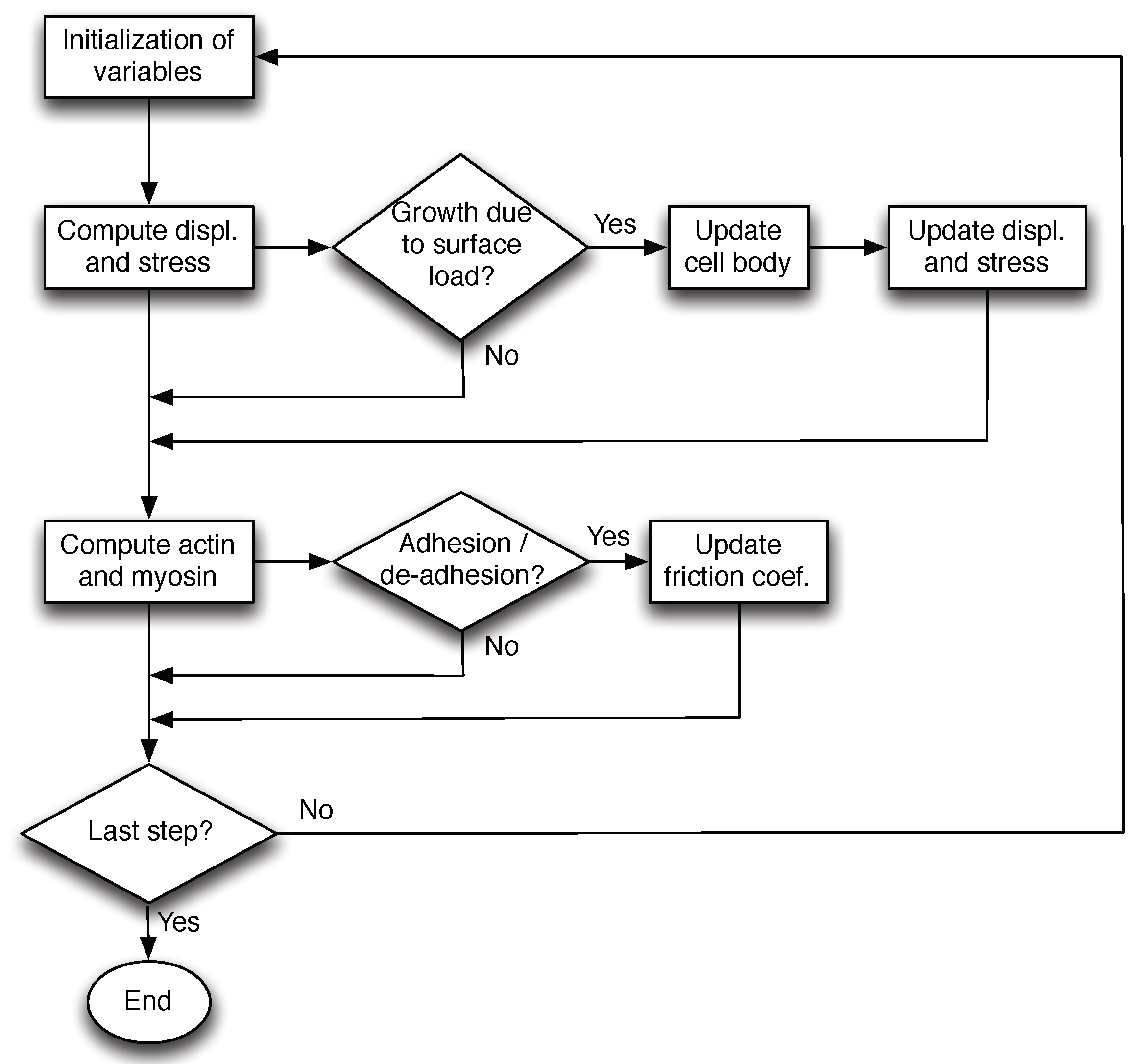
2.2. Numerical Method

In order to solve Equations (3)–(14), we use a suitable finite difference scheme to discretize and numerically compute the solution of the considered problem.

Given initial conditions and choosing uniform space and time discretization, we solve the system at each time step following four steps:

• Firstly, we use the stable Crank–Nicholson scheme to compute the displacement u, and consequently the stress tensor $\sigma$ at each time step through the corresponding constitutive law.
• Secondly, we update the actin and myosin concentrations (bound and free) using a similar scheme.
• If an external stress is applied, the cell is deformed mechanically. If the growth stress threshold ${\sigma }_g$ is reached, the membrane is detached from the actin creating new space and Equations (16) and (17) are solved.
• Finally, after updating the variables, we check if the compression stress threshold ${\sigma }_c$ is reached in order to update the friction coefficient with the substrate $\beta$.

Figure 4 shows a sketch of the numerical method. At each time step, we compute the cell displacement and stress together with the actin and myosin concentrations and we check if some threshold is reached in order to update the corresponding parameters.

3. Results

In this section, we present some numerical results for a cell migration process by solving the model proposed above. Moreover, we carry out a sensitivity analysis in order to justify its applicability.

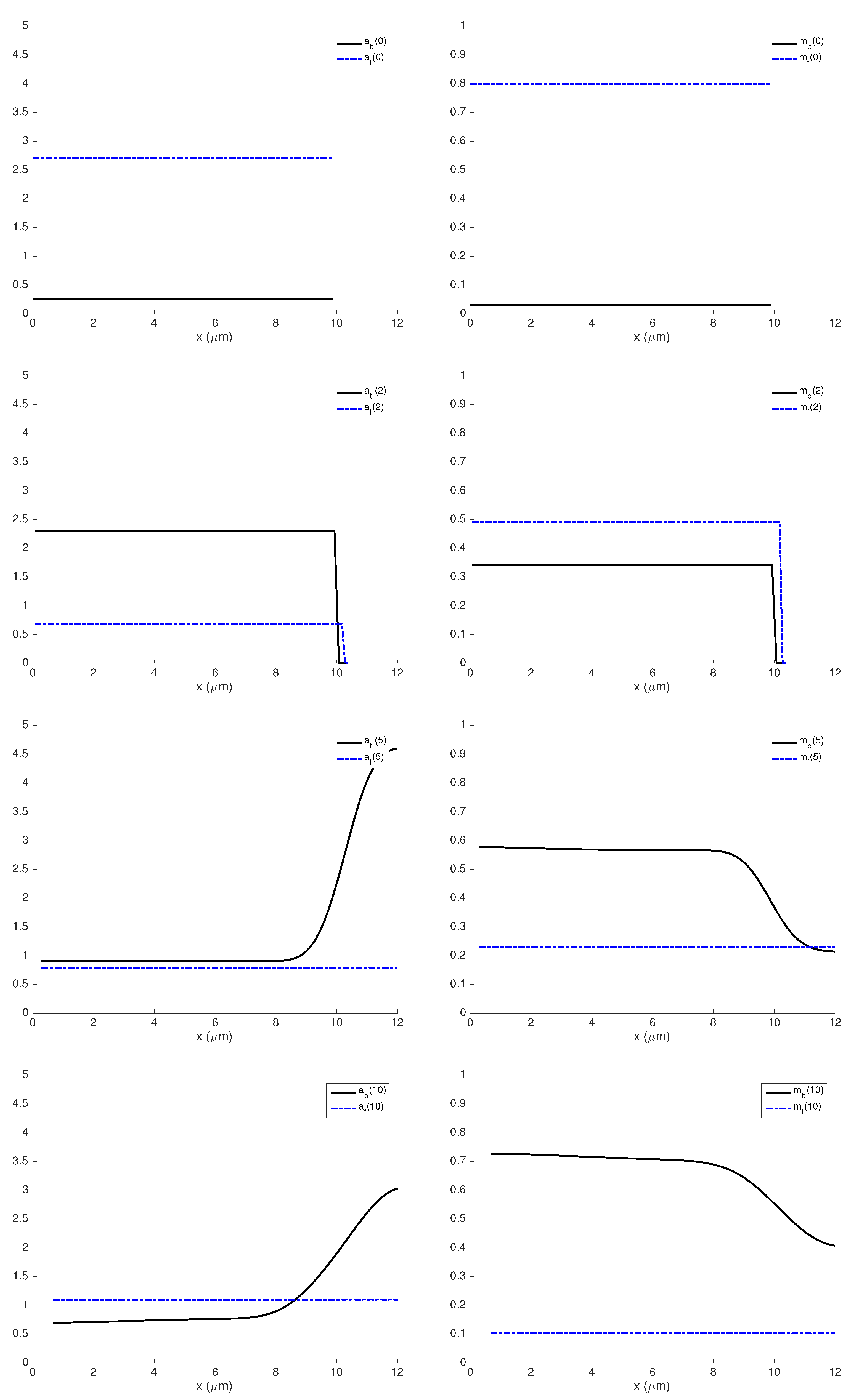
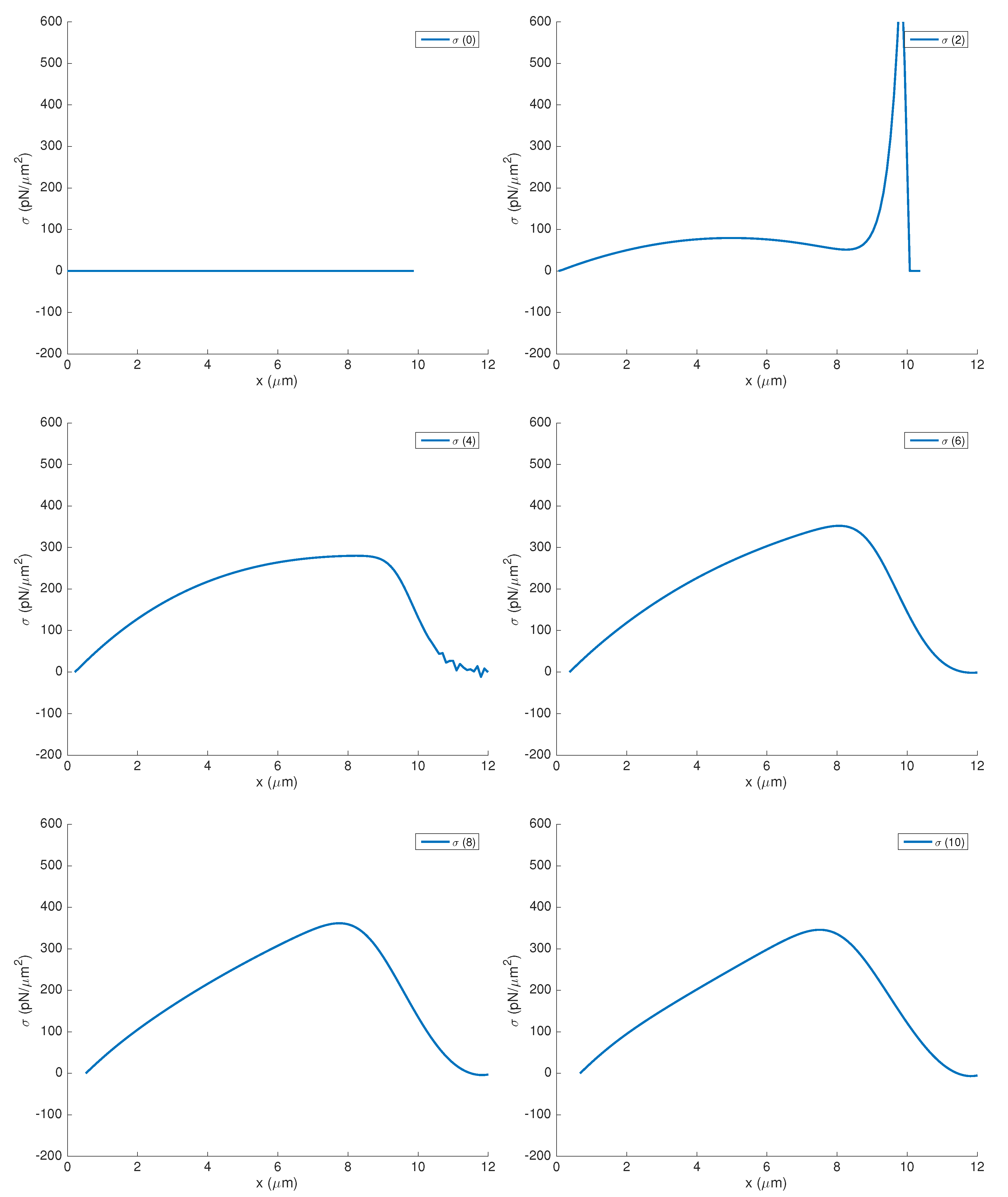
3.1. Influence of Actin and Myosin Densities on Cell Mechanics

In order to evaluate the model, numerical simulations are conducted. The aim of these simulations is to determine the influence of the actin and myosin concentrations on the cell movement and deformation. The values of the parameters used in the model are gathered in

Table 1. Numerical values for the mechanical data and phenomena parameters.

Parameter	Symbol	Value	Source
Substrate friction	$\beta$	103 pNs/µm3	[4]
Reduced substrate friction	${\beta }_c$	10−3 pNs/µm3	Estimated
Initial Young modulus	$E_0$	104 pNs/µm2	[4]
Myosin stress	${\eta }_m$	103 pNs/µm2	[4]
Bound actin and myosin diffusion coefficient	$D_{ab},D_{mb}$	0.1 µm2/s	[4]
Free actin and myosin diffusion coefficient	$D_{af},D_{mf}$	104 µm2/s	Estimated
Activation rate for bound actin	$k_a$	0.067 s−1	[22]
Inactivation rate for bound actin	$\delta$	0.9 s−1	[22]
Bound actin maximal rate	$\gamma$	1 s−1	[22]
Bound actin saturation parameter	K	1 µM	[22]
Activation rate for bound myosin	$k_{mp}$	0.25 s−1	Estimated
Depolymerization rate for bound myosin	$k_{mdp}$	0.02 s−1	Estimated

and

Table 2. Numerical values for the parameters of the simulation.

Parameter	Symbol	Value
Initial length of the cell body	$L_0$	10 µm
Simulation spatial step	$\Delta x$	0.1 µm
Total time of the simulation	T	10 s
Simulation time step	$\Delta t$	0.01 s
Stress threshold for growth	${\sigma }_g$	500 pN
Stress threshold for contraction	${\sigma }_c$	750 pN
Activation time	$t_a$	2 s
Activation stress	${\sigma }_a$	25,000 pN
Deactivation time	$t_d$	2.1 s
Deactivation stress	${\sigma }_d$	500 pN

.

We consider the following initial conditions for displacements and stresses together with actin and myosin concentrations:

$$\begin{array}{c}u(x,0)=u_0=0,\sigma (x,0)={\sigma }_0=0,\mathrm{in}{\Omega }_0,\hfill \\ a_b(x,0)=0.25,a_f(x,0)={\displaystyle \frac{\delta a_b(x,0)}{k_a+\gamma {\displaystyle \frac{a_b{(x,0)}^2}{K^2+a_b{(x,0)}^2}}}},\mathrm{in}{\Omega }_0,\hfill \\ m_f=0.8,m_b=0.03,\mathrm{in}{\Omega }_0.\hfill \end{array}$$

These initial conditions are chosen to start the simulation from an equilibrium state for the different densities at the beginning of the process.

The results obtained for 10 s of simulation are shown in Figure 5 and Figure 6.

Figure 5 shows the time evolution of the actin and myosin concentrations. The bound actin concentration grows with time until the application of the external force $h_a\left(t\right)$. Once this force is applied, the actin density accumulates in the front end of the cell, due to the generation of new space to polymerize, and after it starts to decrease to recover a more uniform concentration. Contrarily, the free actin concentration decreases with time until the application of the external force. In addition, the bound and free myosin shows an opposite behavior. The bound myosin grows with time far from the front end and the free myosin decreases with time during the whole simulation.

Finally, Figure 6 shows the displacement together with the stress undergone by the cell body during the simulation. Note that the deformation of the cell body is due to the myosin contraction effect during the interval $(0,t_a)$; after applying the surface load $h\left(t\right)$, an increase in the deformation is suffered and, consequently, a growth in the cell domain is produced; finally, during the interval $(t_d,T),$ the contraction effect is the responsible for less increase in the cell body length. The final length of the cell body is 10.711 µm, which generates an increase of 0.711 µm in 10 s of simulation.

Moreover, Figure 7 shows the evolution with time of the rear and front ends of the cell body. Note that the migration process continues after the deactivation of the external forces but with a slower speed.

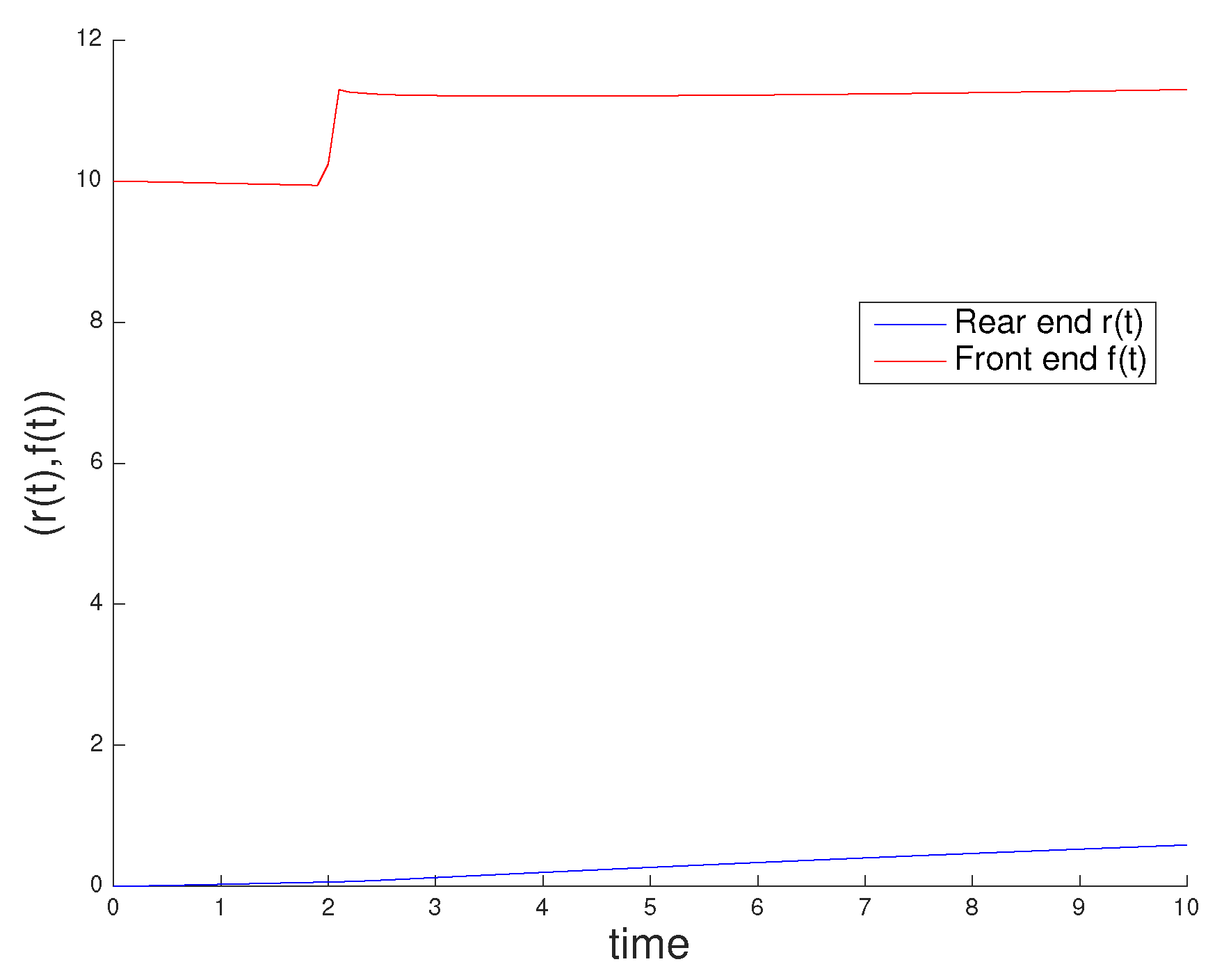
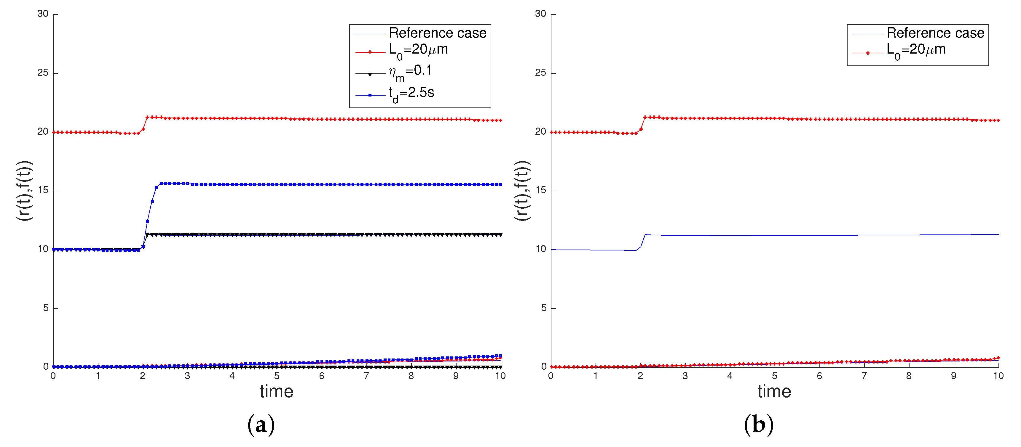
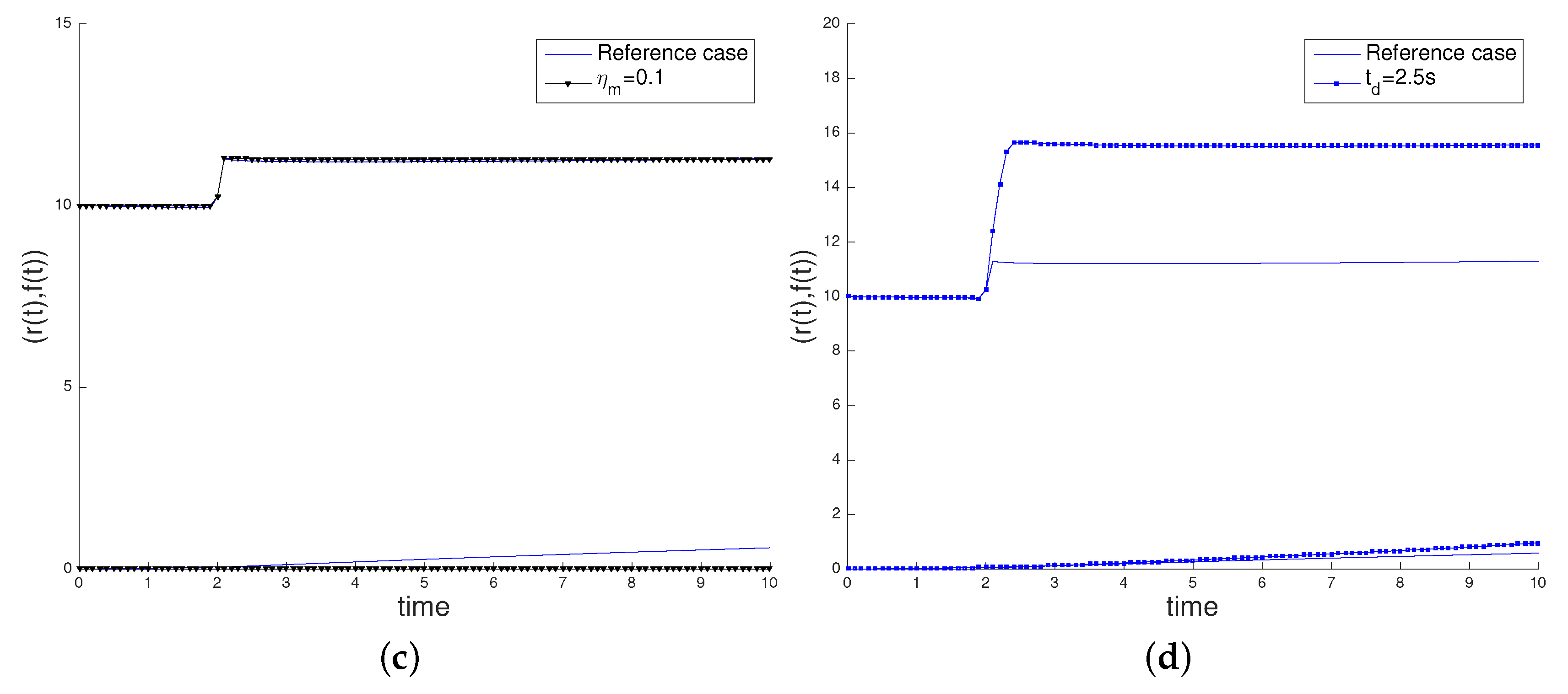
3.2. Sensitivity Analysis

In order to justify the applicability of the model presented here, it is important to analyze the influence of the main phenomena involved in the cell migration process. Due to this, a sensitivity analysis has been carried out, varying some basic parameters in order to better understand the process. We consider the numerical simulation presented in the previous section as the reference case and we analyze the response of the method when varying the following parameters:

• the initial cell length $L_0$, increasing its value to 20 µm,
• the characteristic myosin stress ${\eta }_m$, decreasing its value to 0.1 pN/µm², in order to study the influence of the cell contractility in its movement,
• the time interval of application of the surface load, deactivating the load at $t_d$ = 2.5 s.

Figure 8 shows the results obtained in these three scenarios, comparing them with the results obtained with the reference case. When increasing the initial cell length, the obtained deformation is analogous to the reference case (the cell contracts up to 2 s, then it grows when the surface load is applied, and finally it suffers from a lower increase due to the contraction effect). When the myosin stress ${\eta }_m$ is reduced, the cell barely contracts and the growth in the cell length is greater (1.274 µm in 10 s of simulation). Finally, when delaying the deactivation time from $t_d=2.1$ s to $t_d=2.5$ s, we obtain similar results to the reference case, but the contraction effect is lower and a growth of 4.658 µm is produced.

4. Discussion and Conclusions

In this work, we introduce a one-dimensional mathematical model to simulate the cell deformation and movement during interstitial migration, that is, when the cell is confined in a microfluidic channel. This model allows for studying the behavior of the cell and the proteins involved in the process: free and bound actin and free and bound myosin. It takes into account not only the mechanical deformation undergone by the cell body, but also the evolution of the protein concentrations during the migration process.

Nevertheless, some hypothesis and simplifications are needed in order to reproduce the cell migration process. As a first approach, we consider that this process can be simulated by a one-dimensional mathematical model. Moreover, this model does not take into account the interaction between the cell cytoskeleton and the surrounding fluid in the microfluidic channel (see, for example, [23]). In this work, we focus on the mechanical response of the cell body with respect to the walls and we neglect the effect of the surrounding fluid during the whole process. Finally, the cell body is considered as a unique entity, without distinguishing between the nucleus and the cytosol. Some authors [19,24,25] simulate the cell nucleus separately during the migration process in microfluidics, highlighting the key role of the nucleus deformability in order to generate adhesions and, therefore, to migrate. More recently, some studies show that cell migration also happens in confined environments with limited adhesion, not only with low adhesiveness (see [26,27]), but also in the absence of adhesion complexes (see [28]). Nevertheless, the effect of adhesion and friction with the walls of the device is considered a surface load in the model presented here.

Regarding the numerical results obtained with this model, as expected, we observe that the larger concentration of bound actin monomers is placed in the front end, where traction forces are applied. Contrarily, the bound myosin is mainly located at the rear extreme of the body cell. Regarding the mechanical behavior of the cell, we notice that the maximum stress is reached when the surface force is applied, and, next, the cell attains a more relaxed state. Taking into account the experimental results obtained for interstitial migration in microfluidic devices in [2,29], the obtained results prove that the proposed model reproduce qualitatively the expected behavior of a cell in interstitial migration.

The next step in this model will be the inclusion of the fluid–structure interaction between the cell and the surrounding fluid in the microfluidic devices in order to simulate the process of directional choice when a cell migrates in these types of confined channels.

References