Article

An Energy Landscape Treatment of Decoy Selection in Template-Free Protein Structure Prediction

1
Department of Computer Science, George Mason University, 4400 University Drive, MS 4A5, Fairfax, VA 22030, USA
2
Department of Statistics, George Mason University, 4400 University Drive, MS 4A5, Fairfax, VA 22030, USA
3
Department of Bioengineering, George Mason University, 4400 University Drive, MS 4A5, Fairfax, VA 22030, USA
4
School of Systems Biology, George Mason University, 4400 University Drive, MS 4A5, Manassas, VA 20110, USA
*
Author to whom correspondence should be addressed.
Computation 2018, 6(2), 39; https://doi.org/10.3390/computation6020039
Submission received: 22 April 2018 / Revised: 11 June 2018 / Accepted: 14 June 2018 / Published: 19 June 2018
(This article belongs to the Special Issue Computation in Molecular Modeling)

Abstract

:
The energy landscape, which organizes microstates by energies, has shed light on many cellular processes governed by dynamic biological macromolecules leveraging their structural dynamics to regulate interactions with molecular partners. In particular, the protein energy landscape has been central to understanding the relationship between protein structure, dynamics, and function. The landscape view, however, remains underutilized in an important problem in protein modeling, decoy selection in template-free protein structure prediction. Given the amino-acid sequence of a protein, template-free methods compute thousands of structures, known as decoys, as part of an optimization process that seeks minima of an energy function. Selecting biologically-active/native structures from the computed decoys remains challenging. Research has shown that energy is an unreliable indicator of nativeness. In this paper, we advocate that, while comparison of energies is not informative for structures that already populate minima of an energy function, the landscape view exposes the overall organization of generated decoys. As we demonstrate, such organization highlights macrostates that contain native decoys. We present two different computational approaches to extracting such organization and demonstrate through the presented findings that a landscape-driven treatment is promising in furthering research on decoy selection.

1. Introduction

Increasingly faster and cheaper high-throughput gene sequencing technologies have contributed millions of uncharacterized protein-encoding gene sequences in genomic databases [1]. As of April 2017, the Protein Data Bank (PDB: http://www.rcsb.org/pdb) [2], where wet laboratories deposit resolved biologically-active structures, contains 129 , 553 such structures for slightly over 40 , 000 distinct protein sequences. This disparity highlights the high labor and cost demands of wet-laboratory efforts and motivates the development of complementary, computational approaches to protein structure determination.
Template-free methods, which focus on the most challenging setting of obtaining biologically-active structures of a protein from knowledge of its amino-acid sequence (in absence of a structural template from a close or remote homologous sequence), are improving their capabilities [3]. Popular, representative methods include Rosetta [4] and Quark [5]. These methods operate under the umbrella of stochastic optimization, as they compute structures, also referred to as decoys, by probing local minima of a selected energy/scoring function that sums atomic interactions [6].
Template-free protein structure prediction is a challenging task for various reasons. The protein structure space is vast and continuous; the number of structures in which a sequence of amino acids can fold grows exponentially with the number of amino acids. Any discretization, however, may miss important structures, as the space is continuous; the actual variables selected to represent a structure take values in a continuous range. A distinction is often made between a structure and a conformation to denote the fact that a structure, typically thought of as a placement of atoms in three-dimensional space, may be computationally represented by variables that are not Cartesian coordinates of the constitutive atoms. Such variables can be angles (defined over bonds connecting atoms), or collective variables encoding concerted motions of groups of atoms in three-dimensional space. An instantiation of variables is referred to as a conformation, and kinematics processes (forward versus inverse) are defined to extract a structure from a conformation and vice-versa. We point the interested reader to the review in Ref. [6] for a detailed treatment of variable selection and its importance in protein structure modeling. In protein structure prediction, the variables of choice are the dihedral angles defined over three consecutive bonds. These number in the hundreds or more for small-to-medium proteins (no more than 300 amino acids), and give rise to a high-dimensional conformation space that template-free methods have to explore in their search for biologically-active conformations of an amino-acid sequence.
In addition to challenges related to the size and dimensionality of the search space, it remains unclear what makes a conformation biologically-active/native. Research has shown that energy functions designed and optimized to obtain conformations of a protein sequence are unreliable indicators of nativeness, as it is observed that low energy does not correlate with nativeness; that is, a lower-energy conformation is often not closer to a (known but withheld) native structure [7]. Identifying one or more native conformations from the set of (decoy) conformations computed by a template-free method, a problem also known as decoy selection, remains open in protein structure prediction [8,9].
Decoy selection has garnered its own evaluation category in the Critical Assessment of protein Structure Prediction (CASP) series of community wide experiments [10]. The latest CASP assessment [11] shows that decoy selection remains a bottleneck. Setting an energy threshold either misses native structures or allows the inclusion of too many non-native ones. In light of these findings, a popular approach to decoy selection has been to ignore energy and cluster decoys by their structural similarity [10,12,13]. Once clustering has been performed, the k highest-populated clusters (k varying from 1 to 10), are typically offered as prediction [14].
The utility of an energy-ignoring, clustering-based strategy is tightly related to the quality of the generated decoys, and the strategy has varied success [14]. Specifically, the premise in cluster-based decoy selection is that decoys are randomly distributed around the “true answer”, which a consensus-seeking method should be able to reveal. This premise is flawed for two primary reasons. First, due to the size and dimensionality of the conformation space, the decoy generation process in template-free methods employs heuristics and biases that decidedly steer decoy generation away from a uniformly-sampled view of the conformation space. In addition, energy functions designed for template-free methods contain in them inherent biases that often invalidate entire regions of the conformation space, though such regions may contain native structures. It should be noted that there is often no single true answer, as proteins are intrinsically-dynamic molecules capable of populating distinct structures with which they bind to other molecules. Though in CASP the assessment is with respect to one native structure determined in the wet laboratory, there is a growing consensus that the multiplicity of native structures cannot be ignored [15,16,17,18].
Cluster-based methods fail to pick up exceptionally-good decoys and are especially weak when applied to hard targets, where decoys are typically highly dissimilar (and sparsely sampled) [10]. In response to these findings, two growing thrusts of research focus on designing new, statistical scoring functions that can assess the quality of a single decoy [19,20] and machine learning (ML) methods (often in combination with statistical scoring functions) trained on labeled decoys [21]. These methods have to overcome many challenges, including model generalization and transferability; that is, the ability to be applicable to different decoy data sets. Though in their infancy, these directions are showing promise, and we summarize them in Section 1.1 that reviews related work in decoy selection.
In this paper, in light of outstanding challenges in decoy selection, we highlight a complementary treatment that brings the focus back to the energy landscape view of structural dynamics for intrinsically-dynamic molecules, such as proteins. The energy landscape relates biologically-active conformations of a molecule to thermodynamic stability (and function) [22,23,24,25], and has been central to a better understanding of the relationship between protein structure, dynamics, and function [18,26]. We propose an energy landscape-driven treatment of decoy selection, building on the recognition that in their decoy generation/sampling process template-free methods probe an underlying energy landscape. Specifically, utilizing recent spatial data analytics techniques, we seek and extract local components from the energy landscape sampled/probed during decoy generation by a template-free method. These landscape components, referred to as basins, correspond to the stable and semi-stable conformational states (to the extent that such states are sampled by a template-free method) utilized by a protein to carry out biological activities. Once the decoys are organized into basins, characteristics of basins can then be leveraged for decoy selection via basin selection.
We report on two computational methods and their ability to extract the organization of generated decoys via analysis of the probed energy landscape. The first method has been recently published, and we summarize it here to showcase the ability of an energy landscape-driven treatment to highlight basins containing native conformations. The second method constitutes a novel approach to analysis of generated decoys, and we showcase its ability to provide visual representations of probed landscapes that highlight basins and their relationship with known native structures. These methods are described in Section 4, and their evaluation is presented in Section 2. The paper concludes with a discussion in Section 3, which places the presented findings in context and suggests that a landscape-driven treatment is promising in furthering research on decoy selection.
We first proceed with a more detailed (but by no means exhaustive) overview of related work in decoy selection in Section 1.1 for the interested reader.

1.1. Related Work

Decoy selection literature is rich and features diverse methods that can be grouped into single-model, bag-of-models, quasi-single, and machine learning (ML) methods.
Single-model methods assess the quality of one structure at a time [27,28,29,30] via a scoring that can be physics-based, or knowledge-based. Physics-based scoring functions model specific atomic interactions (e.g., electrostatic, hydrogen bonding, Van Der Waals interactions, and others) [31,32,33]. Knowledge-based functions (also referred to as statistical functions) rely on statistical analysis of known native structures [34,35,36,37,38,39,40,41] and penalize decoy structures where measurements deviate from values observed over known native structures.
Although decoy selection methods utilizing statistical scoring functions have been quite successful and are generally recognized as better able to distinguish native structures from non-natives ones [42,43], some physics-based functions have also been shown effective [44]. However, while both physics-based and statistical scoring functions achieve varied degree of success, none are shown consistent in selecting native structures over non-native ones [45,46,47]. Studies report that the underlying reason behind the apparent ineffectiveness is partially due to the decoy generation process itself not providing enough decoys close to the native structure [48].
Cluster-based decoy selection is the most popular operationalization of the bag-of-models approach for decoy selection. As summarized in Section 1, the basis of cluster-based methods [12,13,49,50,51,52] is the principle of consensus on structural similarity among generated decoys. Although cluster-based methods offer significant improvements over single model-based methods, these strategies encounter a major bottleneck for large decoy sets [53]. If the decoy set includes 100 or more structures, 10 , 000 or more pair-wise distance comparisons would be needed. Several alternative approaches to distance calculations and auxiliary techniques have been proposed to speed up the clustering process [54,55]. Some of these alternative techniques include the concept of partial clustering [56] and geometric constraint propagation [57]. These techniques are able to accelerate the clustering process with or without marginal sacrifice of clustering quality [53,54]. However, cluster-based decoy selection performs poorly when most of the decoys are very different from the known native structure(s), which stems from the basis of a consensus-seeking approach.
Quasi single-model methods adopt strategies from both single-model and bag-of-models methods. These methods first select some high-quality structures as references and then compare the rest of the decoys with the reference structures [29]. Quasi single-model methods are shown to improve decoy selection over single-model and consensus-seeking methods [58,59].
A complementary and rather recent approach in decoy selection makes use of ML models and follows either a single-model or a bag-of-model strategy. These supervised learning models are a-priori trained on expert-constructed structural features [21,60,61] or discriminate by statistical scoring functions [20,62], utilizing models, such as Support Vector Machines [63,64], Neural Network [65,66], Random Forest (RF) [67], and even ensemble methods [21]. Though in their infancy, these methods are showing promise and warrant further evaluation.

2. Results

We present here findings on a test dataset of 10 proteins of different folds and lengths (number of amino acids), as shown in Table 1. For each of these proteins, the amino-acid sequence is used as input for the Rosetta ab-initio protocol [4], and the protocol is executed around 50,000 times in the Mason Argo supercomputing cluster to obtain around 50,000 decoys per protein. Table 1 shows a known native structure (its PDB identifier) for each protein. The native structure is used to evaluate the quality of the basins identified by each of the presented methods. The test cases listed in Table 1 feature easy, medium, and difficult cases for Rosetta. This is a categorization that is made evident by findings reported later in the paper, but that also emerges from expedient analysis in terms of the lRMSD over all decoys from the corresponding native structure; RMSD refers to root-mean-squared-deviation, and lRMSD refers to least RMSD, which is obtained after removing differences due to rigid-body motions (translations and rotations in space). Specifically, the boundaries between the three difficulty levels (easy, medium, hard) are guided by the performance of a cluster-based decoy selection method selected as baseline in this paper.

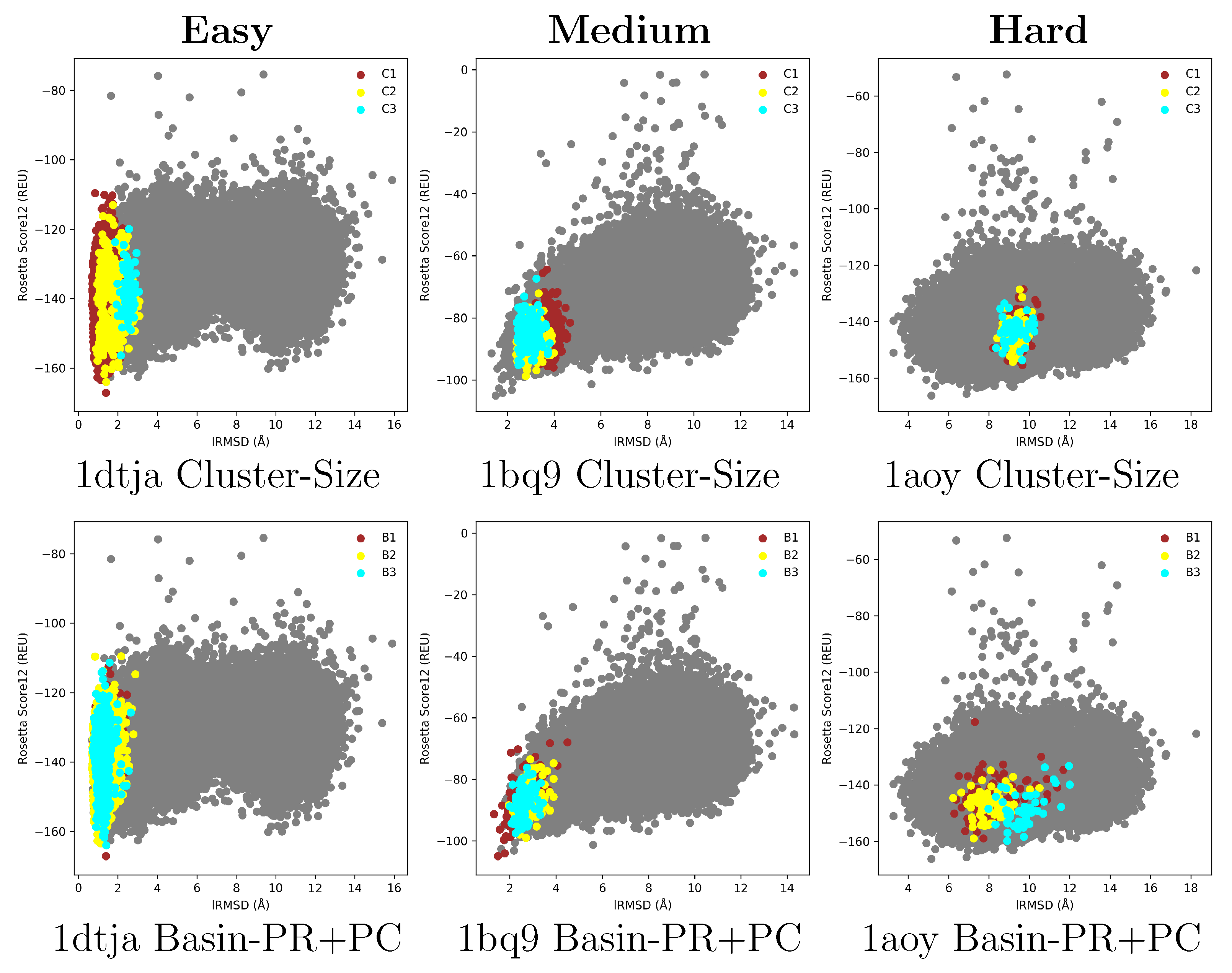
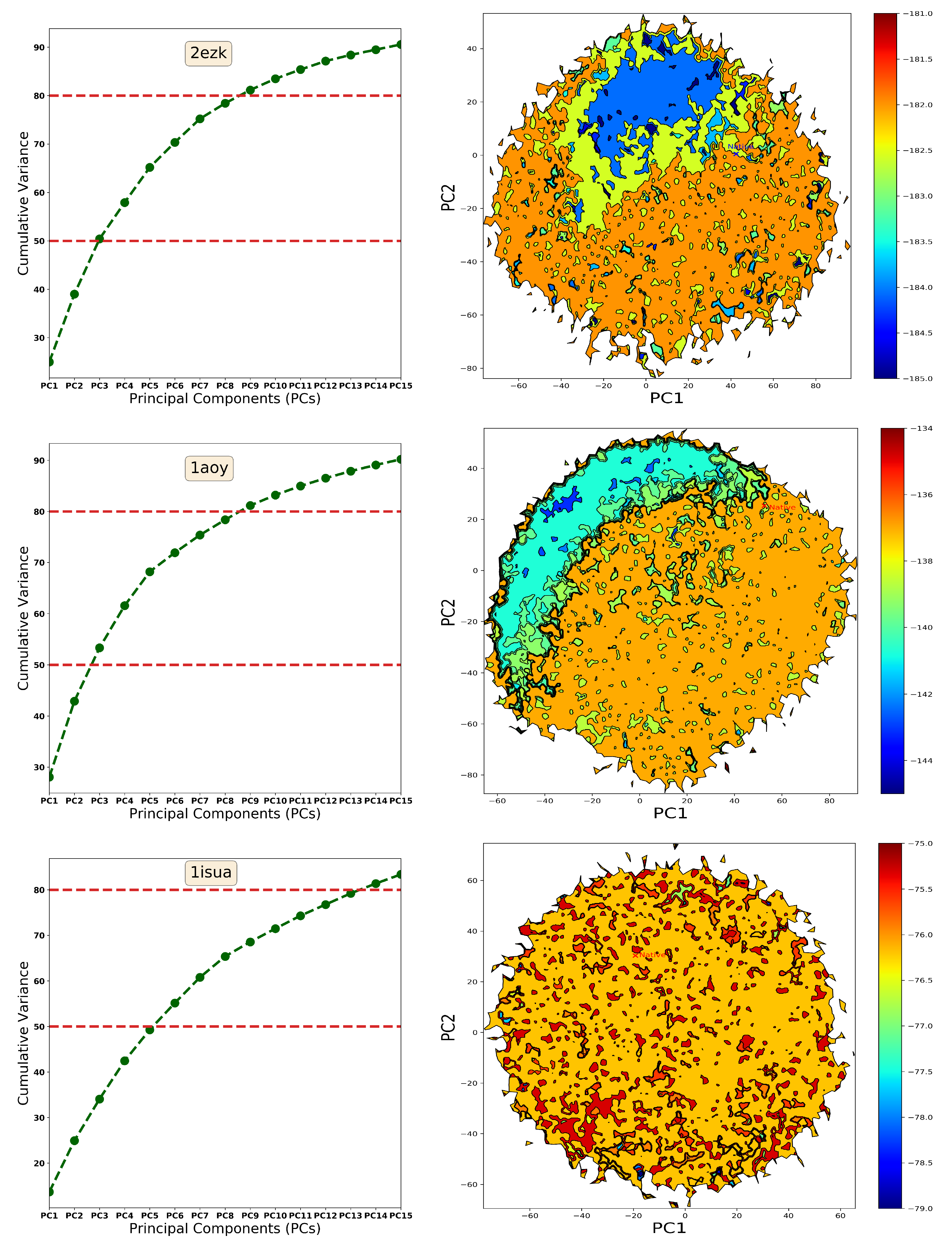
2.1. Summary of Evaluation of Basin Selection for Decoy Selection

Detailed results evaluating the performance of the first method (which identifies and selects basins without reconstructing the landscape) have been recently presented in [68]. Here, we summarize these results to place the contribution of an energy landscape treatment of decoy selection in context. We showcase the best-performing basin selection technique among four techniques investigated in [68]. After identifying basins, various features/measurements can be obtained from the basins and can be employed to rank basins for a selection strategy. Size, the number of decoys mapped to a basin, can be used as a feature to rank basins from the largest to the smallest, and this simple, basin-size strategy, can be used to select the top k basins (k varying from 1 to 3) and compare their quality to the top/largest k clusters picked by a baseline cluster-based method for decoy selection. Other basin selection strategies additionally consider the depth of a basin (the energy of its focal minimum), and even treat basin depth and size as a conflicting optimization objectives in a Pareto-based selection strategy. The latter is referred to as Basin-PR+PC, to indicate that first basins are sorted by their Pareto rank (PR), and then by their Pareto count (PC) to obtain a ranking for selection of the top k basins. The PR and PC measures are often employed in multi-objective optimization in evolutionary computation, and the interested reader is referred to work in [68] for a detailed description and background.
Figure 1 provides a visual comparison of three representative test cases (from easy, medium, and hard targets). Decoys in each of the top 3 groups (clusters or basins) are plotted as dots; the 3 groups are plotted in different clusters. Row 1 in Figure 1 shows results for a baseline, cluster-based method that implements leader clustering, plotting the decoys mapped to the largest 3 clusters. The top 3 basins selected by the Basin-PR+PC basin selection technique are shown in the second row in Figure 1.
Figure 1 provides visual feedback on the ability of basin selection to detect basins closer to the native structure than clusters. This can be quantified via metrics, such as the percentage of near-native conformations (n) in a basin (over the total number of native conformations ), and purity (p), measured as the proportion of native conformations relative to the size of a group (basin or cluster). This metric penalizes a group with a high percentage of true positives (near-native conformations) which also contains a large number of false positives (non-native conformations). The notion of “near-native” indicates that a distance threshold (based on the RMSD metric) is used to determine whether a decoy is close/similar to the native structures (hence, near-native). Analysis in [68] investigates the effect of the distance threshold on the quality of the clusters and basins per these two metrics. In summary, if the lowest lRMSD (over all decoys) min_dist 0.7 (these are the easy cases in Table 1), dist_thresh is set to 2 Å. For medium-difficulty targets ( 0.7 Å <min_dist < 2 Å), dist_thresh varies in 2– 4.5 Å. For the hard cases, where min_dist 2 Å, dist_thresh is set to 6 Å.
Table 2 shows these metrics for the top cluster/basin and the 3 top cluster/basins. Detailed analysis of these results can be found in [68]. In summary, on easy cases, even selecting clusters by size results in high-purity clusters, though basin selection has a more consistent performance over the easy targets. Noticeable improvements in purity are observed for basin selection over clustering on medium and hard targets. For instance, on a medium target, the protein with native structure under PDB entry 1bq9, the top three clusters do not have any decoys with lRMSD < 2 Å (see Figure 1), which in turn results in low purity (p ranges from 1.5 % to 24%). In contrast, Basin-PR+PC achieves improved purity along with decoys with comparatively lower lRMSDs from the native (<2 Å, p ranges from 49.2 % to 80.4 %). The utility of an energy landscape treatment via basin selection is more prominent on the hard targets. For instance, consider the protein with a known native structure under PDB entry 1aoy. Clustering is clearly outperformed by Basin-PR+PC, as the top clusters fail to detect any decoys with lRMSD 8 Å (see Figure 1). In contrast, the top two basins have decoys with lRMSD as low as 6 Å. This visual results conform with the quantitative summary. The purity for the cluster-size-based technique is 0%, whereas Basin-PR+PC achieves purity as high as 43.5 % ( 9.8 % and 5.5 % for 1aoy). As can be seen from the results related in Table 2, purity is higher (indicated in bold) on all test cases in the medium and hard categories for the selected basins than the clusters; we note that purity is expected to decrease when more basins (or clusters) are selected and analyzed together, as the collective number of non-native decoys grows, thus diluting purity. A detailed analysis (not shown here) demonstrates that the results obtained by the basin selection strategies are statistically significantly better in comparison to the results obtained by clustering. In summary, Fisher’s one-sided test [69] is performed on 2 × 2 contigency tables that compare the number of near-native decoys versus the number of non-native decoys in each group (we investigate all three settings, comparing the top basin versus the top cluster, the top two basins versus the top two clusters, and the top three basins versus the top three clusters), in each protein, and in each basin selection strategy in comparison to clustering. The results (of at least one basin selection strategy) are statistically significantly better (p-values < 0.05 ) than clustering at the 95% confidence values for all 9 / 10 targets (the exception being the target with native structure under PDB entry 1isua). On the 9 / 10 targets, where the performance of at least one basin selection strategy is statistically significantly better than the performance of clustering, the obtained p-values range from less than 2.2 × 10 16 to 0.01108 .

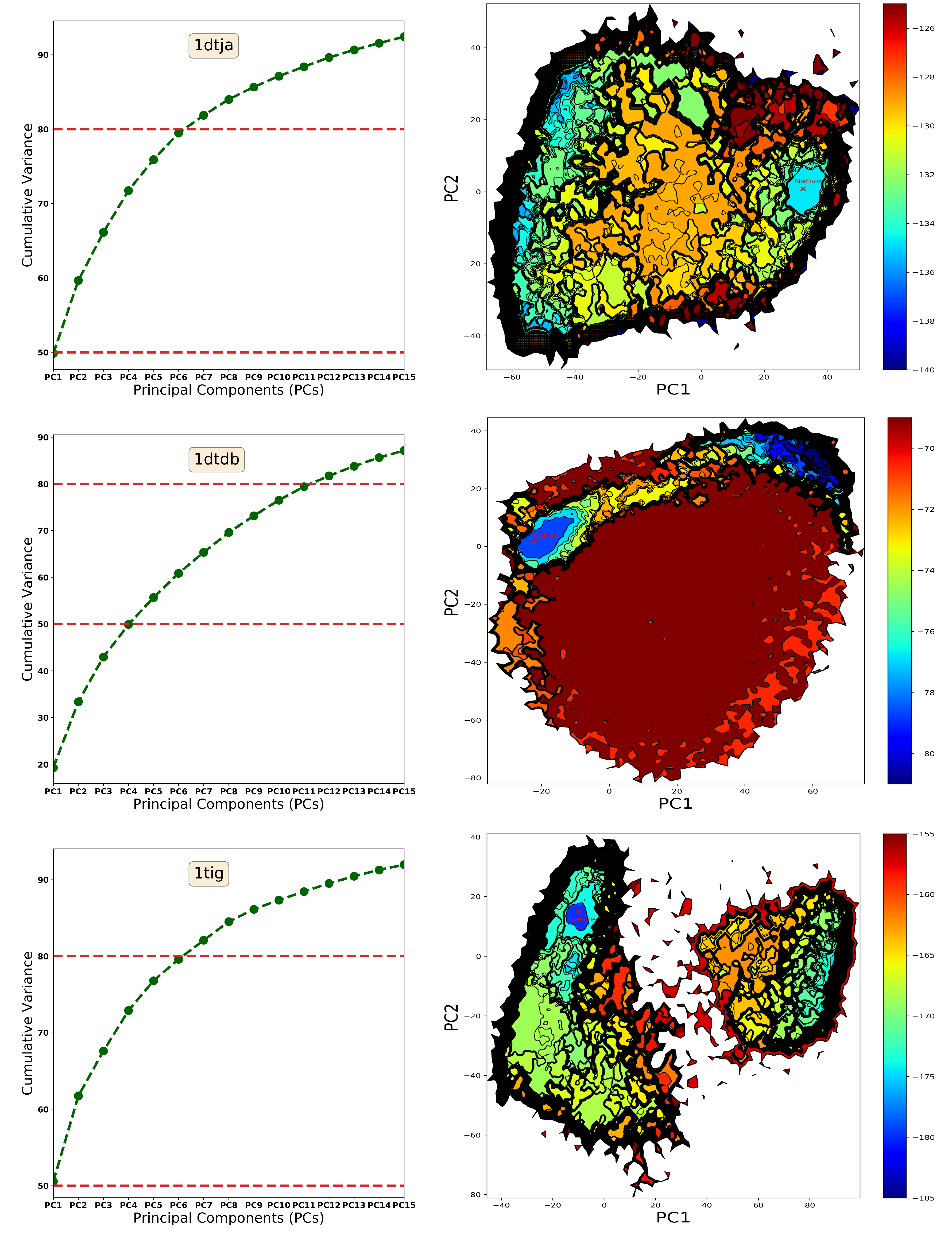
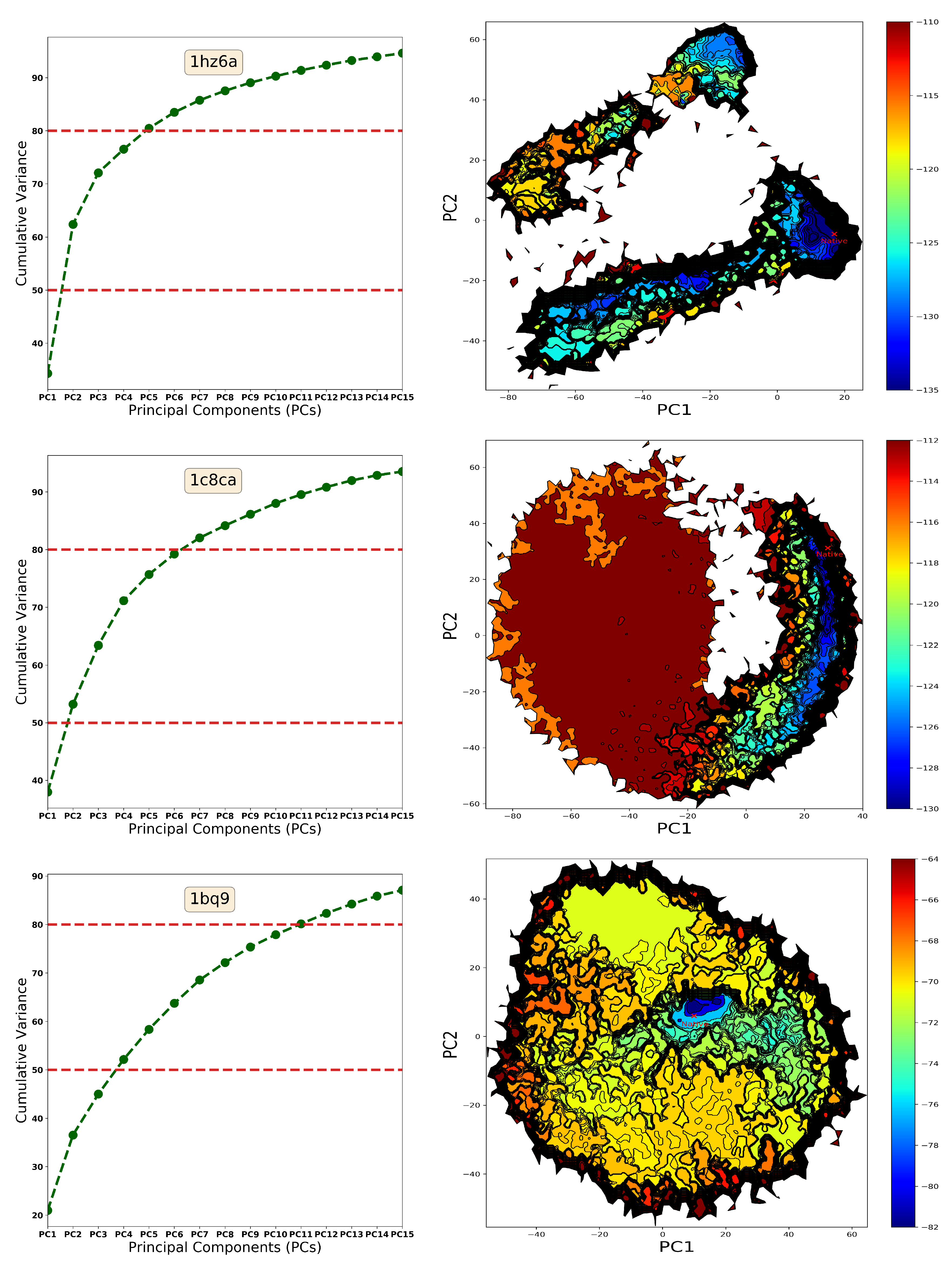
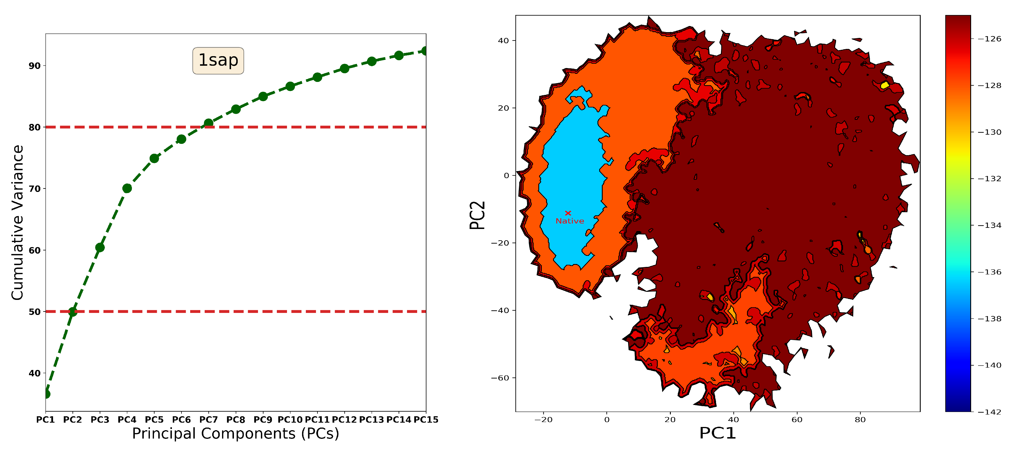
2.2. Summary of Evaluation of Landscape Reconstruction for Decoy Selection

We now show the landscapes reconstructed for each of the 10 protein targets with the method described in Section 4. Figure 2, Figure 3, Figure 4 and Figure 5 show two plots for each protein, the accumulation of variance plot and the actual 2D landscapes (on the PC1-PC2 grid). The accumulation of variance plot shows the cumulative variance obtained by considering more PCs; these plots are limited to the top 15 PCs. Lines are drawn at the 50% threshold to easily indicate how many PCs are needed to achieve this variance, as a way of determining whether the landscapes visualized on two dimensions, PC1 and PC2, capture a major portion of the structural diversity. The landscapes drawn for each target are over the PC1-PC2 grid, with contour lines showing boundaries of basins detected by the landscape reconstruction method. The color coding shows deeper (lower-energy) regions in blue, and higher-energy regions in red. The known native structure for each target is also indicated, based on its projection over PC1 and PC2. The location is marked by a red X.
Figure 2 shows that the native structure available from the PDB for each of the easy protein targets falls on a deep and wide basin. In the case of the protein with a known native structure under PDB entry 1tig, the native structure falls on the deepest basin (row 3 in Figure 2); a large portion of the conformation space is not sampled by the Rosetta decoy generation protocol, as indicated by the white region, perhaps due to the Rosetta energy function steering decoy generation away from that region during optimization. On the other two targets, the basin that colocates in PC1-PC2 space with the known native structure is not the deepest, but it is both low in energy and large in size. This is particularly evident for the protein with a known native structure under PDB entry 1dtja (row 1 in Figure 2). These results explain why basin selection strategies (presented above) have an easy time on these two proteins, particularly when selecting based on both objectives of (large) size and (low energy) per a Pareto-based analysis. On these two targets, the top two PCs capture around 60% of the variance, which confers confidence to conclusions made from visualizations of the reconstructed 2D landscape embeddings.
Row 2 in Figure 2 presents an interesting case. The majority of the space (dark red) is undersampled by the Rosetta decoy generation protocol (few, interspersed conformations with high energies percolate their energies to nearest neighbors on the grid via kernel regression). Moreover, the basin housing the known native structure (PDB entry 1dtdb) is not the deepest. Another region of the landscape (top right) is low in energy and contains many decoys. Visualization of the landscape directly informs on how inherent biases in the Rosetta energy function prefer regions (and so turn them into basins) that may not contain native decoys. The landscape also illustrates why basin selection strategies would have a hard time on this protein, as such strategies may be drawn towards the regions on the top right of the 2D embedding shown in Figure 2).
The cumulative variance captured by the top two PCs varies from 40–60% for the medium targets, as shown in column 1 in Figure 3 and Figure 4. The landscapes also become richer in features. For instance, row 1 in Figure 3 shows (for the protein with a known native structure under PDB entry 1hz6a) a large unsampled region of the conformation space and many small, deep basins, one of which colocates with the known native structure; the latter is not the deepest but is both deep and large, which helps explain why the Pareto-based basin selection strategy presented above, which selects by considering both size and focal energy, does well on this target (high purity in the top basin it selects). Large non- or under-sampled regions can also be seen in row 2 for the protein with a known native structure under PDB entry 1c8ca. There is one region of the conformation space that houses very low-energy structures (see elongated deep/blue basin with many smaller basins inside), and the native structure projects on this region. This is in agreement with the good performance of the Pareto-based basin selection strategy. Similar observations regarding the location of the native structure and the ability of a basin selection strategy to obtain native decoys can be drawn on the protein with a known native structure under PDB entry 1bq9 (row 3 in Figure 3) and the protein with a known native structure under PDB id 1sap. On the latter, the majority of the conformation space is undersampled by Rosetta, with the exception of a well-defined, large, but shallow basin housing the known native structure.
As expected, due to the low quality of decoys generated by Rosetta for the hard cases, results for these proteins decidedly degrade. As can be seen in column 1 in Figure 5, the cumulative variance captured by the top two PCs ranges from the lower 30% to 50%. The location of the native structure does not align with the largest or deepest basin. Though on two of the proteins (rows 1 and 2) Rosetta does prefer specific regions (turning them into basins), on one of them no deep basins can be detected (row 3). On the protein with a known native structure under PDB entry 2ezk, the landscape contains a large and deep basin, but the native structure does not fall in that basin. On the protein with a known native structure under PDB entry 1aoy, basins are shallow, and narrow deep basins exist, again with the native structure very far away. On the protein with a known native structure under PDB entry 1isua, the landscape is overall flat, with no appreciable modularity to indicate the presence of basins.
Overall, the reconstructed landscapes show that a landscape treatment is beneficial in exposing native and near-native basins, particularly on easy and medium targets. On hard targets, the quality of the decoys may limit the ability to detect basins at all, or the captured basins are manifestations of biases in the energy function that steers generated decoys away from native ones. In addition to holding promise for decoy selection, these results also suggest that reconstructions of landscapes is informative to expose under-sampled regions of the conformation space and provide feedback that can be operationalized by decoy generation methods to improve their sampling and, possibly more importantly, their energy functions.

3. Discussion

The findings presented in this paper suggest that an energy landscape treatment of decoy selection is promising and warrants further investigation. Specifically, the study presented in this paper focuses on basins of energy landscapes probed by the decoy generation stage in template-free methods for protein structure prediction. The focus on basins is warranted due to the theoretical, computational, and experimental research that demonstrates that biologically-active structures of a protein, even when diverse, populate basins at the lower-energy regions of the energy landscape.
Specifically, this paper has presented two complementary methods, one where the basins are extracted without reconstruction of the energy landscape, and another where the reconstruction process facilitates extracting the hierarchical organization of basins within basins in protein energy landscapes. While energy is often ignored in favor of structural similarity in cluster-based methods for decoy selection, the presented work indicates that energy can be employed reliably to improve decoy selection. The selection of basins is more effective than the selection of clusters for decoy selection. In particular, considering not just the size but also the energy of a basin in selection is more effective in yielding high-purity basins containing a low number of false positives. The showcased Pareto-based selection strategies demonstrate better performance on a variety of targets that include hard cases with conformation spaces poorly sampled by the Rosetta decoy generation method. Specifically, the improved performance of these strategies suggests that a landscape-based treatment of selecting decoys can lower the number of false positives (non-native decoys) reported.
The findings presented here demonstrate that the improved sampling capability of template-free methods, such as Rosetta, which is utilized here to obtain decoy datasets for diverse protein targets, allows identifying basins that contain native structures for many proteins. As the evaluation in Section 2 highlights, challenging protein targets remain, where the generated decoys are very far away from the native structure.
In cases where the quality of decoys suffers greatly due to shortcomings of the decoy generation stage, the second method described in this paper, provides valuable feedback. By reconstructing the probed energy landscape and providing visual representations of the probed landscape, the method allows visualizing the regions where the decoy generation stage has spent its computational resources. The method exposes directly either under-sampled regions, or overly-sampled regions where the energy function has steered the sampling of decoys. Comparison of such regions with the region that would house a known native structure provides information that can be utilized by decoy generation methods to identify biases in the employed energy function.
The presented work is a first step and opens many lines of future enquiry. While cluster- and basin-based selection strategies are useful for ranking, they do not assess the quality of a single decoy. However, by considering the energy landscape as a whole, the decoys in selected basins provide an informative set that can be assessed by scoring functions to reveal indicators of nativeness. Finally, it is worth noting that the methods described in this paper are general. While the evaluation presented in the paper focuses on the Rosetta all-atom energy landscape, in principle, all the described concepts and techniques extend to landscapes of any scoring function, including statistical scoring functions, including landscapes obtained by other studies beyond the setting of template-free protein structure prediction.

4. Materials and Methods

We first relate concepts regarding energy landscapes that are leveraged in the methods we describe here for extracting the organization of decoys and highlighting native decoys.

4.1. The Energy Landscape

The energy landscape of a protein describes its potential energy as a function of the variables selected to represent protein structures (also referred to as conformational variables) [70]. Conceptually, a point of the landscape corresponds to an energy-evaluated conformation, or a conformation-and-energy pair. The concept of the energy landscape is central to enquiry in diverse scientific disciplines, from the physics of disordered systems such as spin-glasses, to molecular biology [22], to characterization of hard search and optimization problems in Artificial Intelligence [3], and even the broader study of complex systems [71]. In these disciplines, the landscape is referred to as the fitness or the height landscape.
A fitness landscape consists of a set X of points, a neighborhood N ( X ) defined on X, a distance metric on X, and a fitness function f : X R 0 that assigns a fitness to every point x X . Every point in X is assigned a neighborhood by the neighborhood function N. The neighborhood organization of energy landscape unravels the accessibility of one conformation from another. In the context of decoy selection, points x X are decoy conformations, and the fitness function scores the decoys.
Protein energy landscapes are complex. They are multi-dimensional and multimodal. An energy landscape may contain many components or elements, such as basins (or wells) and barriers that separate the basins. The concept of a basin is tied to a local/focal minimum. Specifically, a focal minimum in the landscape is surrounded by a basin of attraction, which is the set of points on the landscape from which steepest descent/ascent converges to that focal optimum. Barriers separate basins and regulate transitions of a system between different conformational states corresponding to basins in the landscape.
In light of the energy landscape, the decoy generation phase in template-free structure prediction methods can be conceptualized as sampling points from an unknown, underlying landscape. That is, at the end of the decoy generation stage, a template-free method has obtained a discrete, sample-based view of the landscape as a set or collection of points on the landscape. It is highly desirable for the decoy generation stage to obtain an unbiased and uniformly-dense view of the landscape, so that obtained decoys cover the multitude of basins possibly present in a protein energy landscape and not miss basins containing native conformations. Please note that we are explicitly stating that there may be many basins containing native conformations, rather than one unique basin. Typically, in protein structure prediction, it is assumed that the native conformational state of a protein is homogeneous and contains similar conformations (corresponding to one basin) [72]. However, there is a growing realization in protein structure modeling and CASP, stemming from many biological studies [73], that one needs to consider the multiplicity of native conformations; that is, a protein may utilize different, biologically-active conformational states that correspond to different basins in the landscape [16]. Despite this realization, the assessment in CASP of template-free methods is conducted with respect to one native structure withheld from the modelers.
Under the energy landscape treatment, one can then in principle identify the possibly different native conformational states by identifying the corresponding basins in the landscape. This presents several challenges. One has to extract the underlying organization of decoys to identify basins in the landscape. We present here two approaches. The first approach embeds the decoys in a connectivity data structure and utilizes energies to identify basins. The second approach explicitly reconstructs the landscape first and provides a visualization that highlights the present basins and the hierarchical organization of basins within basins.
Even if one is able to extract basins with or without reconstructing the underlying energy landscape, there is no guarantee that the present basins contain among them the basin(s) containing native conformations. Ideally, the decoy generation has obtained an unbiased and uniformly-dense view of the landscape; in other words, the decoys cover the different basins. This is often not the case. As summarized in Section 1, because decoy generation proceeds under the umbrella of optimization, it is inherently biased away from high-energy regions in the landscape; more importantly, specific biases in employed energy functions often manifest themselves by steering the decoy generation away from basins that contain native conformations. The second approach that we present in this paper, due to its reconstruction and visualization of the underlying landscape, directly exposes both regions not sampled by decoy generation and non-native basins preferred by decoy generation. We now present each method.

4.1.1. From Decoy Embedding to Basins

Consider an Ω set of decoys generated by a template-free structure prediction method. Research in [74] embeds Ω in a nearest-neighbor graph (nngraph) G = ( V , E ) . The vertex set V is populated with the decoys. The edge set E is populated by inferring the neighborhood structure of the landscape. The distance between two decoys is measured via lRMSD (RMSD after superimposing all decoys to some reference decoy to remove differences due to rigid-body motions). Each vertex u V is connected to vertices v V if d ( u , v ) ϵ , with ϵ being a user-defined parameter. A small ϵ may result in a disconnected graph, which is the result of a sparse, non-uniform sampling of the landscape. This can be remedied by increasing ϵ or the number of nearest neighbors of u.
The vertices of the nngraph G can then be grouped into distinct basins. Because the concept of a basin is tied to its focal minimum, research in [74] first identifies local minima. A vertex u V is a local minimum if v V f ( u ) f ( v ) , where v N ( u ) ( N ( u ) denotes the neighborhood of u). The remaining vertices are then assigned to basins as follows. Each vertex u is associated a negative gradient estimated by selecting the edge ( u , v ) that maximizes the ratio [ f ( u ) f ( v ) ] / d ( u , v ) . From each vertex u that is not a local minimum, the negative gradient is iteratively followed (i.e., the edge that maximizes the above ratio is followed) until a local minimum is reached. Vertices that via this process reach the same local minimum are assigned to the basin associated with that minimum.
This approach, presented first in [74] can be considered an on-graph clustering approach that extracts the basins without reconstructing the underlying landscape. The basins are mutually-exclusive sets of decoys. In [68], we show that the basins extracted in this manner can be useful for decoy selection. Namely, we propose different basin selection strategies (such as, selecting the largest, or the deepest basin, and other selection strategies) and show that the basins selected in this manner are more pure (contain more native than non-native conformations) and outperform methods that cluster decoys based on structural similarity. In addition, in [68], we show that a Pareto-based selection that considers both basin size and depth as conflicting objectives is a superior strategy that selects pure (with more native than non-native decoys) basins even on challenging proteins with low quality of generated decoys. We summarize some of these findings in Section 2, but focus primarily on novel results obtained with a complementary method that reconstructs the landscape to visually expose hierarchical basins, as we describe below.

4.1.2. From Landscape Reconstruction to Basins

A complementary method to exposing basins in the landscape relies on explicitly reconstructing the landscape. Conceptually, the method “fills in” regions of the landscape via kernel regression, which infers energies of points on the landscape based on energies of sampled points (decoys) that are nearest neighbors. Because landscapes are multi-dimensional and continuous, this filling in is limited to points on a grid, which in our preliminary investigation presented in this paper we limit to a grid of two dimensions. That is, the method seeks to reconstruct a lower-dimensional representation of the landscape that utilizes two conformational “coordinates” and the height/fitness coordinate (which tracks energies/scores).
The method extracts the reduced conformational coordinates from statistical analysis of the decoys generated by a template-free structure prediction method. Specifically, for the evaluation presented in this paper, the method utilizes Principal Component Analysis (PCA) [75] to extract collective, variance-preserving coordinates from decoy structures. PCA and other linear dimensionality reduction techniques are shown effective for analysis of protein structures in various applications of interest in computational biology [16,76,77].
The method leverages an analysis of the cumulative variance to assess when the top two Principal Components (PCs) provide effective, reduced conformational coordinates; as we relate in Section 2, this is the case on many of the protein targets studied in this paper. Via this mechanism, generated decoys are reduced to two-dimensional points on a PC1-PC2 space.
Given a representation of each decoy as a two-dimensional point, the method then computes the alpha convex hull containing the points (corresponding to decoys) via the method described in [78,79]. A grid (over PC1 and PC2) is then defined over points in the hull. Energies of grid points are estimated via a bounded-support Gaussian kernel that sums energy contributions from decoys that are nearest neighbors of a grid point. The kernel effectively smooths the landscape and addresses, albeit locally, the non-uniform sampling density of decoys by decoy generation.
Once energies of grid points have been estimated, a recursive process then follows to find basins and exposes the hierarchical organization of basins in the landscape. A horizontal line is swept, starting from the maximum energy (over grid points), over levels d E apart, till the minimum energy (over grid points) is reached. At every level, the set of decoys with energies at or below that level are passed on to the alpha convex hull reconstruction technique, which recognizes when boundaries have been split, thus recognizing large basins splitting into new ones. When basin splitting occurs, the method recursively proceeds to analyze those basins in the same fashion, sweeping a line until no points remain, and detecting further basin splitting when separate hull boundaries emerge.
This process captures the hierarchical organization of basins in an energy landscape; that is, that smaller, deeper basins may be contained in larger, shallower basins. This hierarchical organization can be easily visualized, directly relating the basins and the barriers separating them, as related in Section 2. The visualization elucidates regions undersampled or oversampled by a decoy generation technique, providing direct information in inherent biases of a decoy generation technique and/or the energy function utilized by the technique. As we show in Section 2, for many proteins, a native structure available from a wet-laboratory technique is located in a deep and wide basin, providing evidence of the great strides made by decoy generation techniques and thus the premise for the presented method. For other proteins, however, the basin preferred by a decoy generation technique is shown to be far away from available native structures. Even in such cases, the results obtained by the proposed method are informative, as they provide direct feedback on the bias of the energy function employed in decoy generation that can be leveraged to further improve the decoy generation process itself.

4.2. Implementation Details

The Structural Biology Library (SBL) [74] is used to obtain basins in the first method, with all parameters set to default values. In the second method, the parameter for the α -convex shape is set to 0.15 , the distance between adjacent grid points varies from 0.1 to 0.3 (based on the density of sampling by the Rosetta decoy generation protocol), and the sweeping line sweeps over energy levels δ 2 = 0.3 units apart. The basin selection techniques operating over basins obtained with SBL and the landscape reconstruction method have been implemented in Python. Each method, using 4 cores and 8 GB memory per core, takes between 26 min and up to 2.5 h over decoy data sets of around 50,000 decoys for proteins ranging in length from 53 to 93 amino acids.

Author Contributions

All authors contributed equally to the conceptualization and design of the methodologies presented here. N.A. led method implementation and evaluation. A.S. and N.A. wrote the manuscript with assistance from W.Q.

Funding

This research was funded by the National Science Foundation Grant No. 1421001 to A.S. and a Jeffress Memorial Trust Award to W.Q. and A.S.

Acknowledgments

Computations were run on ARGO, a research computing cluster provided by the Office of Research Computing at George Mason University.

Conflicts of Interest

The authors declare no conflict of interest.

Abbreviations

The following abbreviations are used in this manuscript:
PDBProtein Data Bank
CASPCritical Assessment of protein Structure Prediction
lRMSDleast root-mean-squared-deviation
MLMachine Learning
NNNeural Network
Random ForestRF
PCPareto Count
PRPareto Rank
SVMSupport Vector Machines

References

  1. Blaby-Haas, C.E.; de Crécy-Lagard, V. Mining high-throughput experimental data to link gene and function. Trends Biotechnol. 2013, 29, 174–182. [Google Scholar] [CrossRef] [PubMed]
  2. Berman, H.M.; Henrick, K.; Nakamura, H. Announcing the worldwide Protein Data Bank. Nat. Struct. Biol. 2003, 10, 980. [Google Scholar] [CrossRef] [PubMed]
  3. Shehu, A. A Review of Evolutionary Algorithms for Computing Functional Conformations of Protein Molecules. In Computer-Aided Drug Discovery; Zhang, W., Ed.; Springer: New York, NY, USA, 2015. [Google Scholar]
  4. Leaver-Fay, A.; Tyka, M.; Lewis, S.M.; Lange, O.F.; Thompson, J.; Jacak, R.; Kaufman, K.W.; Renfrew, P.D.; Smith, C.A.; Sheffler, W.; et al. ROSETTA3: An object-oriented software suite for the simulation and design of macromolecules. Methods Enzymol. 2011, 487, 545–574. [Google Scholar] [PubMed]
  5. Xu, D.; Zhang, Y. Ab initio protein structure assembly using continuous structure fragments and optimized knowledge-based force field. Proteins Struct. Funct. Bioinform. 2012, 80, 1715–1735. [Google Scholar] [CrossRef] [PubMed]
  6. Shehu, A. Probabilistic Search and Optimization for Protein Energy Landscapes. In Handbook of Computational Molecular Biology; Chapman & Hall/CRC Computer & Information Science Series; Aluru, S., Singh, A., Eds.; CRC Press: London, UK, 2013. [Google Scholar]
  7. Verma, A.; Schug, A.; Lee, K.H.; Wenzel, W. Basin hopping simulations for all-atom protein folding. J. Chem. Phys. 2006, 124, 044515. [Google Scholar] [CrossRef] [PubMed]
  8. Kryshtafovych, A.; Fidelis, K.; Tramontano, A. Evaluation of model quality predictions in CASP9. Proteins 2011, 79, 91–106. [Google Scholar] [CrossRef] [PubMed] [Green Version]
  9. Kryshtafovych, A.; Barbato, A.; Fidelis, K.; Monastyrskyy, B.; Schwede, T.; Tramontano, A. Assessment of the assessment: Evaluation of the model quality estimates in CASP10. Proteins 2014, 82, 112–126. [Google Scholar] [CrossRef] [PubMed]
  10. Moult, J.; Fidelis, K.; Kryshtafovych, A.; Schwede, T.; Tramontano, A. Critical assessment of methods of protein structure prediction (CASP)—Round X. Proteins Struct. Funct. Bioinform. 2014, 82, 109–115. [Google Scholar] [CrossRef] [PubMed]
  11. Moult, J.; Fidelis, K.; Kryshtafovych, A.; Schwede, T.; Tramontano, A. Critical Assessment of Methods of Protein Structure Prediction (CASP)—Round XII. Proteins 2017. [Google Scholar] [CrossRef] [PubMed]
  12. Ginalski, K.; Elofsson, A.; Fischer, D.; Rychlewski, L. 3D-Jury: A simple approach to improve protein structure predictions. Bioinformatics 2003, 19, 1015–1018. [Google Scholar] [CrossRef] [PubMed]
  13. Wallner, B.; Elofsson, A. Identification of correct regions in protein models using structural, alignment, and consensus information. Protein Sci. 2006, 15, 900–913. [Google Scholar] [CrossRef] [PubMed] [Green Version]
  14. Molloy, K.; Saleh, S.; Shehu, A. Probabilistic Search and Energy Guidance for Biased Decoy Sampling in Ab-initio Protein Structure Prediction. IEEE/ACM Trans. Bioinform. Comp. Biol. 2013, 10, 1162–1175. [Google Scholar] [CrossRef] [PubMed]
  15. Shehu, A.; Plaku, E. A Survey of omputational Treatments of Biomolecules by Robotics-inspired Methods Modeling Equilibrium Structure and Dynamics. J. Artif. Intell. Res. 2016, 597, 509–572. [Google Scholar]
  16. Maximova, T.; Moffatt, R.; Ma, B.; Nussinov, R.; Shehu, A. Principles and Overview of Sampling Methods for Modeling Macromolecular Structure and Dynamics. PLoS Comp. Biol. 2016, 12, e1004619. [Google Scholar] [CrossRef] [PubMed]
  17. Shehu, A.; Clementi, C.; Kavraki, L.E. Sampling Conformation Space to Model Equilibrium Fluctuations in Proteins. Algorithmica 2007, 48, 303–327. [Google Scholar] [CrossRef]
  18. Okazaki, K.; Koga, N.; Takada, S.; Onuchic, J.N.; Wolynes, P.G. Multiple-basin energy landscapes for large-amplitude conformational motions of proteins: Structure-based molecular dynamics simulations. Proc. Natl. Acad. Sci. USA 2006, 103, 11844–11849. [Google Scholar] [CrossRef] [PubMed] [Green Version]
  19. Zhao, F.; Xu, J. A position-specific distance-dependent statistical potential for protein structure and functional study. Structure 2012, 20, 1118–1126. [Google Scholar] [CrossRef] [PubMed]
  20. He, J.; Zhang, J.; Xu, Y.; Shang, Y.; Xu, D. Protein structural model selection based on protein-dependent scoring function. Stat. Interface 2012, 5, 109–115. [Google Scholar] [CrossRef]
  21. Mirzaei, S.; Sidi, T.; Keasar, C.; Crivelli, S. Purely Structural Protein Scoring Functions Using Support Vector Machine and Ensemble Learning. IEEE/ACM Trans. Comput. Biol. Bioinform. 2016, 1–14. [Google Scholar] [CrossRef] [PubMed]
  22. Bryngelson, J.D.; Onuchic, J.N.; Socci, N.D.; Wolynes, P.G. Funnels, pathways, and the energy landscape of protein folding: A synthesis. Proteins Struct. Funct. Bioinform. 1995, 21, 167–195. [Google Scholar] [CrossRef] [PubMed] [Green Version]
  23. Ma, B.; Kumar, S.; Tsai, C.; Nussinov, R. Folding funnels and binding mechanisms. Protein Eng. 1999, 12, 713–720. [Google Scholar] [CrossRef] [PubMed] [Green Version]
  24. Tsai, C.; Kumar, S.; Ma, B.; Nussinov, R. Folding funnels, binding funnels, and protein function. Protein Sci. 1999, 8, 1181–1190. [Google Scholar] [CrossRef] [PubMed] [Green Version]
  25. Tsai, C.; Ma, B.; Nussinov, R. Folding and binding cascades: Shifts in energy landscapes. Proc. Natl. Acad. Sci. USA 1999, 96, 9970–9972. [Google Scholar] [CrossRef] [PubMed] [Green Version]
  26. Nussinov, R.; Wolynes, P.G. A second molecular biology revolution? The energy landscapes of biomolecular function. Phys. Chem. Chem. Phys. 2014, 16, 6321–6322. [Google Scholar] [CrossRef] [PubMed]
  27. Uziela, K.; Wallner, B. ProQ2: Estimation of model accuracy implemented in Rosetta. Bioinformatics 2016, 32, 1411–1413. [Google Scholar] [CrossRef] [PubMed]
  28. Liu, T.; Wang, Y.; Eickholt, J.; Wang, Z. Benchmarking deep networks for predicting residue-specific quality of individual protein models in CASP11. Sci. Rep. 2016, 6, 19301. [Google Scholar] [CrossRef] [PubMed]
  29. Jing, X.; Wang, K.; Lu, R.; Dong, Q. Sorting protein decoys by machine-learning-to-rank. Sci. Rep. 2016, 6, 31571. [Google Scholar] [CrossRef] [PubMed] [Green Version]
  30. Wallner, B.; Elofsson, A. Can correct protein models be identified? Protein Sci. 2003, 12, 1073–1086. [Google Scholar] [CrossRef] [PubMed] [Green Version]
  31. Brooks, B.R.; Bruccoleri, R.E.; Olafson, B.D.; States, D.J.; Swaminathan, S.; Karplus, M. CHARMM: A program for macromolecular energy, minimization, and dynamics calculations. J. Comput. Chem. 1983, 4, 187–217. [Google Scholar] [CrossRef]
  32. Cornell, W.D.; Cieplak, P.; Bayly, C.I.; Gould, I.R.; Merz, K.M.; Ferguson, D.M.; Spellmeyer, D.C.; Fox, T.; Caldwell, J.W.; Kollman, P.A. A second generation force field for the simulation of proteins, nucleic acids, and organic molecules. J. Am. Chem. Soc. 1995, 117, 5179–5197. [Google Scholar] [CrossRef]
  33. Jorgensen, W.L.; Tirado-Rives, J. The OPLS [optimized potentials for liquid simulations] potential functions for proteins, energy minimizations for crystals of cyclic peptides and crambin. J. Am. Chem. Soc. 1988, 110, 1657–1666. [Google Scholar] [CrossRef] [PubMed]
  34. McConkey, B.J.; Sobolev, V.; Edelman, M. Discrimination of native protein structures using atom–atom contact scoring. Proc. Natl. Acad. Sci. USA 2003, 100, 3215–3220. [Google Scholar] [CrossRef] [PubMed]
  35. Samudrala, R.; Moult, J. An all-atom distance-dependent conditional probability discriminatory function for protein structure prediction1. J. Mol. Biol. 1998, 275, 895–916. [Google Scholar] [CrossRef] [PubMed]
  36. Lu, H.; Skolnick, J. A distance-dependent atomic knowledge-based potential for improved protein structure selection. Proteins Struct. Funct. Bioinform. 2001, 44, 223–232. [Google Scholar] [CrossRef] [PubMed]
  37. Berrera, M.; Molinari, H.; Fogolari, F. Amino acid empirical contact energy definitions for fold recognition in the space of contact maps. BMC Bioinform. 2003, 4, 8. [Google Scholar] [CrossRef] [Green Version]
  38. Simons, K.T.; Ruczinski, I.; Kooperberg, C.; Fox, B.A.; Bystroff, C.; Baker, D. Improved recognition of native-like protein structures using a combination of sequence-dependent and sequence-independent features of proteins. Proteins Struct. Funct. Bioinform. 1999, 34, 82–95. [Google Scholar] [CrossRef] [Green Version]
  39. Bahar, I.; Jernigan, R.L. Inter-residue potentials in globular proteins and the dominance of highly specific hydrophilic interactions at close separation. J. Mol. Biol. 1997, 266, 195–214. [Google Scholar] [CrossRef] [PubMed]
  40. Reva, B.A.; Finkelstein, A.V.; Sanner, M.F.; Olson, A.J. Residue-residue mean-force potentials for protein structure recognition. Protein Eng. 1997, 10, 865–876. [Google Scholar] [CrossRef] [PubMed] [Green Version]
  41. Miyazawa, S.; Jernigan, R.L. An empirical energy potential with a reference state for protein fold and sequence recognition. Proteins Struct. Funct. Bioinform. 1999, 36, 357–369. [Google Scholar] [CrossRef] [Green Version]
  42. Park, B.; Levitt, M. Energy functions that discriminate X-ray and near-native folds from well-constructed decoys. J. Mol. Biol. 1996, 258, 367–392. [Google Scholar] [CrossRef] [PubMed]
  43. Felts, A.K.; Gallicchio, E.; Wallqvist, A.; Levy, R.M. Distinguishing native conformations of proteins from decoys with an effective free energy estimator based on the opls all-atom force field and the surface generalized Born solvent model. Proteins Struct. Funct. Bioinform. 2002, 48, 404–422. [Google Scholar] [CrossRef] [PubMed]
  44. Lazaridis, T.; Karplus, M. Discrimination of the native from misfolded protein models with an energy function including implicit solvation. J. Mol. Biol. 1999, 288, 477–487. [Google Scholar] [CrossRef] [PubMed] [Green Version]
  45. Thomas, P.D.; Dill, K.A. Statistical potentials extracted from protein structures: How accurate are they? J. Mol. Biol. 1996, 257, 457–469. [Google Scholar] [CrossRef] [PubMed]
  46. Ben-Naim, A. Statistical potentials extracted from protein structures: Are these meaningful potentials? J. Chem. Phys. 1997, 107, 3698–3706. [Google Scholar] [CrossRef]
  47. Moult, J. Comparison of database potentials and molecular mechanics force fields. Curr. Opin. Struct. Biol. 1997, 7, 194–199. [Google Scholar] [CrossRef]
  48. Bradley, P.; Chivian, D.; Meiler, J.; Misura, K.; Rohl, C.A.; Schief, W.R.; Wedemeyer, W.J.; Schueler-Furman, O.; Murphy, P.; Schonbrun, J.; et al. Rosetta predictions in CASP5: Successes, failures, and prospects for complete automation. Proteins Struct. Funct. Bioinform. 2003, 53, 457–468. [Google Scholar] [CrossRef] [PubMed]
  49. Lorenzen, S.; Zhang, Y. Identification of near-native structures by clustering protein docking conformations. Proteins Struct. Funct. Bioinform. 2007, 68, 187–194. [Google Scholar] [CrossRef] [PubMed]
  50. Shortle, D.; Simons, K.T.; Baker, D. Clustering of low-energy conformations near the native structures of small proteins. Proc. Natl. Acad. Sci. USA 1998, 95, 11158–11162. [Google Scholar] [CrossRef] [PubMed] [Green Version]
  51. Zhang, Y.; Skolnick, J. SPICKER: A clustering approach to identify near-native protein folds. J. Comput. Chem. 2004, 25, 865–871. [Google Scholar] [CrossRef] [PubMed]
  52. Estrada, T.; Armen, R.; Taufer, M. Automatic selection of near-native protein-ligand conformations using a hierarchical clustering and volunteer computing. In Proceedings of the First ACM International Conference on Bioinformatics and Computational Biology, Niagara Falls, NY, USA, 2–4 August 2010; pp. 204–213. [Google Scholar]
  53. Li, S.C.; Ng, Y.K. Calibur: A tool for clustering large numbers of protein decoys. BMC Bioinform. 2010, 11, 25. [Google Scholar] [CrossRef] [PubMed]
  54. Zhang, J.; Xu, D. Fast algorithm for clustering a large number of protein structural decoys. In Proceedings of the IEEE International Conference on Bioinformatics and Biomedicine, Atlanta, GA, USA, 12–15 November 2011; pp. 30–36. [Google Scholar]
  55. Li, S.C.; Bu, D.; Li, M. Clustering 100,000 protein structure decoys in minutes. IEEE/ACM Trans. Comput. Biol. Bioinform. (TCBB) 2012, 9, 765–773. [Google Scholar]
  56. Zhou, J.; Wishart, D.S. An improved method to detect correct protein folds using partial clustering. BMC Bioinform. 2013, 14, 11. [Google Scholar] [CrossRef] [PubMed]
  57. Berenger, F.; Zhou, Y.; Shrestha, R.; Zhang, K.Y. Entropy-accelerated exact clustering of protein decoys. Bioinformatics 2011, 27, 939–945. [Google Scholar] [CrossRef] [PubMed] [Green Version]
  58. He, Z.; Alazmi, M.; Zhang, J.; Xu, D. Protein structural model selection by combining consensus and single scoring methods. PLoS ONE 2013, 8, e74006. [Google Scholar] [CrossRef] [PubMed]
  59. Pawlowski, M.; Kozlowski, L.; Kloczkowski, A. MQAPsingle: A quasi single-model approach for estimation of the quality of individual protein structure models. Proteins Struct. Funct. Bioinform. 2016, 84, 1021–1028. [Google Scholar] [CrossRef] [PubMed]
  60. Qiu, J.; Sheffler, W.; Baker, D.; Noble, W.S. Ranking predicted protein structures with support vector regression. Proteins Struct. Funct. Bioinform. 2008, 71, 1175–1182. [Google Scholar] [CrossRef] [PubMed]
  61. Ray, A.; Lindahl, E.; Wallner, B. Improved model quality assessment using ProQ2. BMC Bioinform. 2012, 13, 224. [Google Scholar] [CrossRef] [PubMed]
  62. Zhou, H.; Skolnick, J. GOAP: A generalized orientation-dependent, all-atom statistical potential for protein structure prediction. Biophys. J. 2011, 101, 2043–2052. [Google Scholar] [CrossRef] [PubMed]
  63. Cao, R.; Wang, Z.; Wang, Y.; Cheng, J. SMOQ: A tool for predicting the absolute residue-specific quality of a single protein model with support vector machines. BMC Bioinform. 2014, 15, 120. [Google Scholar] [CrossRef] [PubMed]
  64. Chatterjee, S.; Ghosh, S.; Vishveshwara, S. Network properties of decoys and CASP predicted models: A comparison with native protein structures. Mol. BioSyst. 2013, 9, 1774–1788. [Google Scholar] [CrossRef] [PubMed]
  65. Nguyen, S.P.; Shang, Y.; Xu, D. DL-PRO: A novel deep learning method for protein model quality assessment. In Proceedings of the International Joint Conference on Neural Networks (IJCNN), Beijing, China, 6–11 July 2014; pp. 2071–2078. [Google Scholar]
  66. Faraggi, E.; Kloczkowski, A. A global machine learning based scoring function for protein structure prediction. Proteins Struct. Funct. Bioinform. 2014, 82, 752–759. [Google Scholar] [CrossRef] [PubMed]
  67. Manavalan, B.; Lee, J.; Lee, J. Random forest-based protein model quality assessment (RFMQA) using structural features and potential energy terms. PLoS ONE 2014, 9, e106542. [Google Scholar] [CrossRef] [PubMed]
  68. Akhter, N.; Shehu, A. From Extraction of Local Structures of Protein Energy Landscapes to Improved Decoy Selection in Template-free Protein Structure Prediction. Molecules 2017, 23, 216. [Google Scholar] [CrossRef] [PubMed]
  69. Fisher, R.A. On the interpretation of χ2 from contingency tables, and the calculation of P. J. R. Stat. Soc. 1922, 85, 87–94. [Google Scholar] [CrossRef]
  70. Frauenfelder, H.; Sligar, S.G.; Wolynes, P.G. The energy landscapes and motion on proteins. Science 1991, 254, 1598–1603. [Google Scholar] [CrossRef] [PubMed]
  71. Samoilenko, S. Fitness Landscapes of Complex Systems: Insights and Implications On Managing a Conflict Environment of Organizations. Complex. Organ. 2008, 10, 38–45. [Google Scholar]
  72. Shehu, A. Conformational Search for the Protein Native State. In Protein Structure Prediction: Method and Algorithms; Rangwala, H., Karypis, G., Eds.; Wiley Book Series on Bioinformatics: Fairfax, VA, USA, 2010; Chapter 21. [Google Scholar]
  73. Boehr, D.D.; Nussinov, R.; Wright, P.E. The role of dynamic conformational ensembles in biomolecular recognition. Nat. Chem. Biol. 2009, 5, 789–796. [Google Scholar] [CrossRef] [PubMed] [Green Version]
  74. Cazals, F.; Dreyfus, T. The structural bioinformatics library: Modeling in biomolecular science and beyond. Bioinformatics 2017, 33, 997–1004. [Google Scholar] [CrossRef] [PubMed]
  75. Luenberger, D.G. Introduction to Linear and Nonlinear Programming; Addison-Wesley: Boston, MA, USA, 1973. [Google Scholar]
  76. Clausen, R.; Shehu, A. A Data-driven Evolutionary Algorithm for Mapping Multi-basin Protein Energy Landscapes. J. Comput. Biol. 2015, 22, 844–860. [Google Scholar] [CrossRef] [PubMed]
  77. Pandit, R.; Shehu, A. A Principled Comparative Analysis of Dimensionality Reduction Techniques on Protein Structure Decoy Data. In Proceedings of the International Conference on Bioinformatics and Computational Biology, Las Vegas, NV, USA, 4–6 April 2016; Ioerger, T., Haspel, N., Eds.; ISCA: Winona, MN, USA, 2016; pp. 43–48. [Google Scholar]
  78. Rodriguez-Casal, H. Set estimation under convexity type assumptions. Ann. l’Inst. Henri Poincare (B) Probab. Stat. 2007, 43, 763–774. [Google Scholar] [CrossRef]
  79. Pateiro-Lopez, B. Set Estimation under Convexity Type Restrictions. Ph.D. Thesis, Universidad de Santiago de Compostela, Galicia, Spain, 2008. [Google Scholar]
Figure 1. Visualization of selected clusters (first row) and basins (second row) for representative targets with native structures under PDB entries 1dtja, 1bq9, and 1aoy. Decoys are plotted by their least RMSD (after removing rigid-body motions) from the structure in the PDB entry (x axis) and their Rosetta score12 all-atom energy measured Rosetta Energy Units—REUs (y axis).
Computation 06 00039 g001
Figure 2. Results are shown the easy targets. The left panel shows the accumulation of variance for the PCs obtained from PCA of generated decoys. The right panel shows the reconstructed landscape over the PC1-PC2 grid. The contour lines show the basin boundaries. The location of a known native structure for each target protein from the easy category highlighted here is marked by a red X.
Computation 06 00039 g002
Figure 3. Results are shown the medium targets. The left panel shows the accumulation of variance for the PCs obtained from PCA of generated decoys. The right panel shows the reconstructed landscape over the PC1-PC2 grid. The contour lines show the basin boundaries. The location of a known native structure for each target protein from the easy category highlighted here is marked by a red X.
Computation 06 00039 g003
Figure 4. Results for medium targets continued.
Computation 06 00039 g004
Figure 5. Results are shown the hard targets. The left panel shows the accumulation of variance for the PCs obtained from PCA of generated decoys. The right panel shows the reconstructed landscape over the PC1-PC2 grid. The contour lines show the basin boundaries. The location of a known native structure for each target protein from the easy category highlighted here is marked by a red X.
Computation 06 00039 g005
Table 1. Testing dataset (* denotes proteins with a predominant β fold and a short helix). Column 2 shows the PDB ID of a known native structure for each protein. Columns 3 and 4 show the fold and the length (in terms of the number of amino acids), respectively. Column 5 shows the actual size of the decoy set Ω generated via Rosetta for each target protein. Column 6 shows the lowest lRMSD, among all decoys, from the known native structure.
PDB IDFoldLength | Ω | min_dist (Å)
Easy 1 . 1dtdb α + β 61 57 , 839 0.51
2 . 1tig α + β 88 52 , 099 0.60
3 . 1dtja α + β 74 53 , 526 0.68
Medium 4 . 1hz6a α + β 64 57 , 474 0.72
5 . 1c8ca β *64 53 , 322 1.08
6 . 1bq9 β 53 53 , 663 1.30
7 . 1sap β 66 51 , 209 1.75
Hard 8 . 2ezk α 93 50 , 192 2.56
9 . 1aoy α 78 52 , 218 3.26
10 . 1isua c o i l 62 60 , 360 5.53
Table 2. Comparison of cluster-based and basin-based selection strategies.
1dtdb1tig1dtja1hz6a1c8ca1bq91sap2ezk1aoy1isua
Cluster-SizeC 1 n:97.6%n:57.3%n:95.5%n:0%n:10%n:0.6%n:0%n:0%n:0%n:0%
p:99.9%p:99.1%p:99.2%p:0%p:32.1%p:1.5%p:0%p:0%p:0%p:0%
s:22.3%s:8.7%s:21.6%s:4.4%s:3.4%s:0.64%s:9.3%s:0.02%s:0.03%s:0.02%
C 1 3 n:97.6%n:88.4%n:97.8%n:26.4%n:20.5%n:21%n:55.9n:0%n:0%n:0%
p:93.3%p:98.4%p:97.2%p:27.7%p:36.3%p:24%p:7.4p:0%p:0%p:0%
s:23.9%s:13.6%s:22.6%s:10.8%s:6.2%s:1.4%s:17.4%s:0.07%s:0.06%s:0.05%
Basin-PR+PCB 1 n:85.3%n:28.8%n:19.9%n:55.5%n:14%n:9.3%n:32.4%n:1.02%n:0.18%n:0%
p:99%p:100%p:99.6%p:85.5%p:96.3%p:80.4%p:20.2%p:45.9%p:9.8%p:0%
s:19.7%s:4.4%s:4.5%s:7.3%s:1.6%s:0.18%s:3.7%s:0.29%s:0.2%s:0.05%
B 1 3 n:95.4%n:42.8%n:70.7%n:55.5%n:23.5%n:22.7%n:51.4%n:2.0%n:0.23%n:0.03%
p:98.8%p:98.8%p:99.2%p:39.3%p:58.5%p:74.3%p:11.5%p:39.7%p:5.5%p:1.2%
s:22%s:6.6%s:16%s:16%s:4.4%s:0.46%s:10.3%s:0.66%s:0.46%s:0.14%

