Numerical Study on Sloshing Characteristics with Reynolds Number Variation in a Rectangular Tank

Abstract

A study on sloshing characteristics in a rectangular tank, which is horizontally excited with a specific range of the Reynolds number, is approached numerically. The nonlinearity of sloshing flow is confirmed by comparing it with the linear solution based on the potential theory, and the time series results of the sloshing pressure are analyzed by Fast Fourier Transform (FFT) algorithm. Then, the pressure fluctuation phenomena are mainly observed and the magnitude of the amplitude spectrum is compared. The results show that, when the impact pressure is generated, large pressure fluctuation in a pressure cycle is observed, and the effects of the frequencies of integral multiples when the fundamental frequency appears dominantly in the sloshing flow.

1. Introduction

When a partially filled tank is subjected to disturbances from external sources, the liquid inside it undergoes motion called sloshing. Sloshing is an interesting and important phenomenon with wide engineering applications and is of enormous practical and industrial interest. It has been studied in the fields of sea transport (marine vehicles, LNG cargo etc.), land-transport (bulk cargo carriers etc.), air transport (rockets, space vehicles etc.) [1], and areas such as civil (storage tanks, dams etc.), chemical (industry, reactors, etc.), mechanical and nuclear engineering (nuclear vessels, nuclear reactors, etc.) [2]. To address these issues, over the past few decades classification societies, such as Det Norske Veritas (DNV), Bureau Veritas (BV), American Bureau of Shipping (ABS) and Lloyd’s Register (LR), have conducted extensive research and provided guidelines for assessing sloshing loads and safety design [3,4].

Many researchers have studied sloshing in tanks or containers. Kim [5] numerically studied sloshing flows with impact loads in 2D and 3D liquid containers by using the finite difference method (FDM). Chen and Nokes [6] analyzed fully nonlinear and viscous fluid sloshing in a rectangular tank by applying time independent FDM. Wu et al. [7] utilized time independent FDM and numerically studied fluid sloshing in a 3D rectangular tank subjected to horizontal excitation. Arafa [8] developed a finite element method (FEM) to analyze sloshing effects in partially filled rigid rectangular tanks subjected to base excitation. Mitra et al. [9] used FEM to study the sloshing phenomena of inviscid fluids in 2D rectangular, vertically mounted annular cylindrical, trapezoidal, and horizontal circular cylindrical tanks. Nayak and Biswal [10] studied the seismic behavior of a partially filled rectangular tank with a bottom-mounted submerged block by utilizing FEM. Chen et al. [11] numerically simulated liquid sloshing in a partially filled rectangular tank under horizontal harmonic motion with different fill levels and excitation frequencies. Akyildiz and Unal [12] numerically and experimentally investigated sloshing in a 3D rectangular tank by applying the VOF method to assess pressure variations and 3D effects. These numerical studies showed good agreement with experimental and analytical solutions. Likewise, the numerical approaches based on the VOF method have been applied to various phenomena which are difficult to estimate utilizing potential theory, such as strong nonlinear sloshing with separation flow, complex geometries, significant viscosity effects and gas entrainment.

The sloshing phenomena can be generally classified into two kinds of fluid flow. One is the linear sloshing flow which can be analyzed by an analytical approach, such as potential or perturbation theory. The other is the nonlinear sloshing flow, which has strong nonlinearity such as breaking waves. In particular, violent sloshing flow, which accompanies strong nonlinearity, is mostly impossible to assess by an analytical approach and requires experimental or numerical methods for analysis. Since the sloshing pressure patterns become very complex due to nonlinearity or the mixed flow, which has density difference between gas and liquid, a numerical method has been widely adopted for analysis.

Chen et al. [6] and Li et al. [13] conducted the study using the FFT technique for analyzing complex sloshing patterns more quantitatively. This research method seems to reflect well the physical phenomena of sloshing flow quantitatively. Recent studies [6,14] on the sloshing phenomena considering the Reynolds number have been conducted. Chen et al. [6] showed almost linearly increasing peaks of free-surface level with low Reynolds numbers, in the range from Re = 2 × 10³ to 1.6 × 10⁴. The results were analyzed by the FFT technique and compared quantitatively with the magnitude of amplitude spectrum. Birknes-Berg and Pedersen [14] conducted a study on the treatment of boundary layers on a solitary sloshing wave, and the results were analyzed with boundary layer thickness in the range of Re = 1 × 10¹⁰. However, this paper provides the specific boundary layer flow variation with Reynolds number changes on the sloshing flow.

Likewise, the study on the sloshing impact and its flow shapes, when excited with some specific ranges of Reynolds numbers, is very rare. Thus, the purpose of this study is to understand the pressure fluctuation of sloshing and the wave breaking phenomena due to the nonlinearity of relatively high Reynolds numbers. The calculated pressure patterns of sloshing behavior were quantitatively analyzed by the FFT technique.

2. Analysis Model and Methods

2.1. Computational Domain and Boundary Conditions

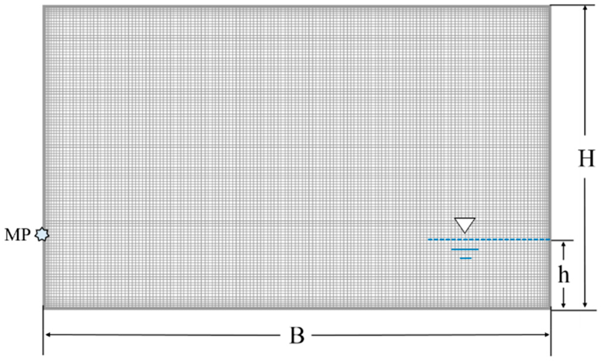
In this numerical study, a two dimensional rectangular tank with a water filing level of 15% of the breadth (B) is considered as a numerical model, and its mesh field is shown in Figure 1. The sloshing phenomena have been simulated using the ANSYS CFX 16.2. The VOF method is used to perform the multi-phase flow analysis between water and air. The k-ω turbulence model is used to analyze the sloshing phenomena near the wall. The high resolution and the Second Order Backward Euler transient schemes are used to discretize convective and time terms, respectively. The rectangular tank is subjected to horizontal excitation by a sinusoidal wave equation:

$$x(t)=A\sin ({\omega }_{n}t)$$

(1)

where A, t, and ω are the amplitude, time, and the natural frequency, respectively. The n-th natural frequency correlation [15] is given by

$${\omega }_n=\sqrt{g{k}_n\tanh \left(k_{n}h\right)}$$

(2)

where g is the gravitational acceleration and mode number n is 1. The k_n is n-th wave number, nπ/B, and the sloshing simulation in the rectangular tank is carried out under the unsteady state and horizontal excitation for all cases. The ideal gas properties of air are considered and the density of water is 998 kg/m³. The front and back sides of the numerical model have symmetric boundary conditions and horizontal motion is considered for periodic excitation. The checking position of sloshing pressure on the wall, MP, is located at 0.15 m from the bottom of the tank, which is the same as the free surface level. Here, B = 1 m, h = 0.15 m and H = 0.6 m.

To understand the influence of the Reynolds number on sloshing phenomena, a total of five cases ranging from Re = 1.8 × 10⁴ to 7.2 × 10⁴ were considered, as shown in

Table 1. Computational conditions for sloshing impact analysis.

Case	Reynolds No.	Natural Frequency (ω1, s−1)	Excited Frequency (Hz)
1	1.8 × 104	3.68	0.586
2	2.5 × 104
3	3.6 × 104
4	5.0 × 104
5	7.2 × 104

. The Reynolds number definition [16] is given by

$$\mathrm{Re}= \frac{{\rho }_{w}A{\omega }_{1}B}{{\mu }_w}$$

(3)

where the ρ_w and μ_w are water density and dynamic viscosity of water, respectively.

2.2. Governing Equations

The VOF method is used for simulating the sloshing flow in the tank subjected to horizontal excitation. Godderidge et al. [17] have compared homogeneous and inhomogeneous multiphase models for sloshing flow in a rectangular tank subjected to sway excitation, and they pointed out that the inhomogeneous model is more suitable for sloshing flow analysis. Thus, even though the inhomogeneous model is more time-consuming than the homogeneous model, we adopted the inhomogeneous model which is well known as reasonable method for sloshing simulation.

Volume Conservation equation:

The total volume fraction is given by

$${\displaystyle \sum _{\alpha }^{N_p}{r}_{\alpha }=1}$$

(4)

The conservation equation between phases is given by

$${\displaystyle \sum _{\alpha }\frac{\partial (r_{\alpha }{U}_{{\alpha }_i})}{\partial x_i}=0}$$

(5)

Continuity equation:

The continuity equation is given by

$$\frac{\partial }{\partial t}\left(r_{\alpha }{\rho }_{\alpha }\right)+\frac{\partial }{\partial x_i}\left(r_{\alpha }{\rho }_{\alpha }{U}_{{\alpha }_i}\right)={\displaystyle {\displaystyle \sum }_a^{N_p}}{\mathsf{\Gamma }}_{\alpha \beta }$$

(6)

Momentum equation:

The momentum equation is given by

$$\begin{array}{l}\frac{\partial }{\partial t}\left(r_a{\rho }_{\alpha }{U}_{\alpha }\right)+\frac{\partial }{\partial x_i}\left(r_{\alpha }\left({\rho }_{\alpha }{U}_{{\alpha }_i}{U}_{{\alpha }_j}\right)\right)\\ =-r_{\alpha }\nabla {\rho }_{\alpha }+\frac{\partial }{\partial x_i}(r_{\alpha }{\mu }_{\alpha }(\nabla U_{ai}+{(\nabla U_{ai})}^T))+{\displaystyle {\displaystyle \sum }_{\beta =1}^{N_p}}({\mathsf{\Gamma }}_{\alpha \beta }^{+}{U}_{\beta }-({\mathsf{\Gamma }}_{\beta \alpha }^{+}{U}_{\alpha }))\end{array}$$

(7)

where N_p is the total number of phases, α and β are phases, r is the fixed volume fraction, U is the velocity, p is the pressure and i, j denotes the tensor. The third term in the right hand side of Equation (7) is the factor that distinguishes between the homogeneous and inhomogeneous models. Γ⁺ indicates the positive mass flow rate per unit volume, and the Γ_αβ is given by

$${\mathsf{\Gamma }}_{\alpha \beta }={\stackrel{.}{m}}_{\alpha \beta }{A}_{\alpha \beta }$$

(8)

where the ${\stackrel{.}{m}}_{\alpha \beta }$ is the mass flow rate per unit interfacial area from phases α and β, and A_αβ is the interfacial area proportional to the volume fraction density. The interfacial area of the free surface model is given by

$$A_{\alpha \beta }=\left|\nabla r_a\right|$$

(9)

2.3. Analytical Solution for Linear Sloshing

The linear analytical solution is based on the potential flow theory established by Faltinsen [18]. It is widely used for validating numerical models of rectangular tank sloshing problems under horizontally excited motions [19,20]. The free surface elevation η can be expressed as [17,18]

$$\eta =\frac{1}{g}{\frac{\partial \mathsf{\Phi }}{\partial t}|}_{y=0},$$

(10)

where

$$\begin{gathered} {\frac{\partial \mathsf{\Phi }}{\partial t}|}_{y=0}={\displaystyle {\displaystyle \sum }_{n=0}^{\infty }}\sin \left[\frac{\left(2n+1\right)\pi }{B}x\right]\cos \left[\frac{\left(2n+1\right)\pi }{B}h\right] \\ \times [-A_n{\omega }_n\sin \left({\omega }_{n}t\right)-C_n{\omega }_n\sin \left(\omega t\right)]-\frac{1}{g}Ax\sin \left(\omega t\right) \end{gathered}$$

(11)

$${\omega }_n^2=g\frac{\left(2n+1\right)\pi }{B}\tanh \left[\frac{\left(2n+1\right)\pi }{B}h\right]$$

(12)

$$A_n=-C_n-\frac{K_n}{\omega }$$

(13)

$$C_n=\frac{\omega K_n}{{\omega }_n^2-{\omega }_n}$$

(14)

$$K_n=\frac{\omega A}{\cos \mathrm{h}[\frac{(2n+1)\pi }{B}h]}\frac{2}{a}[\frac{B}{(2n+1)\pi }{]}^2{(-1)}^n$$

(15)

2.4. Discussion of the Numerical Model with Inhomogeneous VOF

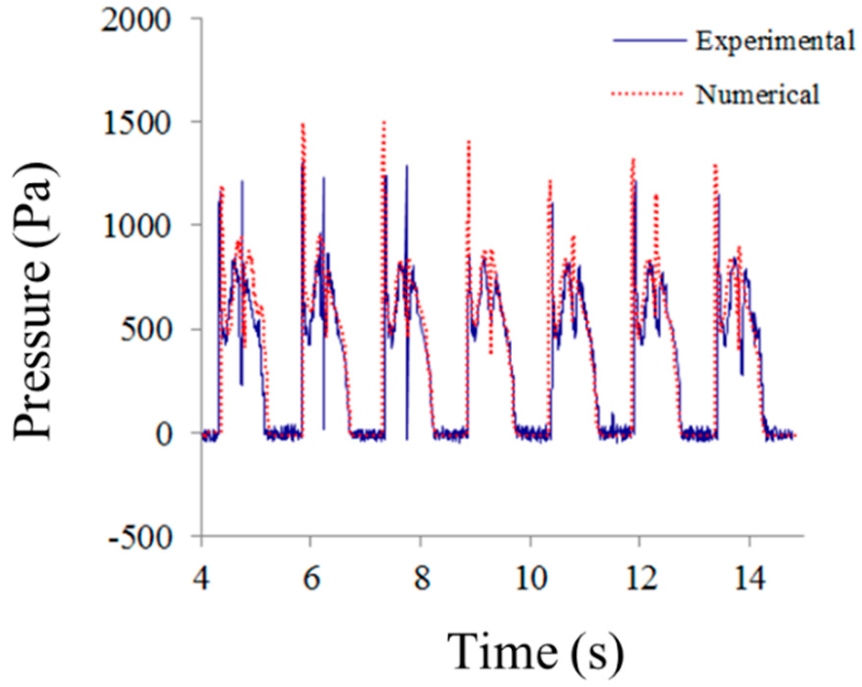
Validation of this numerical model with inhomogeneous VOF has been carried out by Parthasarathy et al. [21] and Kim et al. [22], using the experimental results obtained by Kishev et al. [23]. Figure 2 shows the time histories of pressure on the wall. The peak pressures are calculated to be 5% to 10% higher than the experimental data during seven periods. The numerical results are in agreement with the experimental data.

3. Results and Discussion

The results show the sloshing pressure variations for 0 to 30 s under the Reynolds number ranges as shown in Table 1, and the visualized shapes of sloshing flow at the moment of peak pressure for each condition. The time-historically calculated sloshing pressure data were analyzed by the FFT technique. The magnitude of amplitude spectrum and the components of frequencies were quantitatively compared using FFT results.

3.1. Observing Nonlinearity of Sloshing Flows

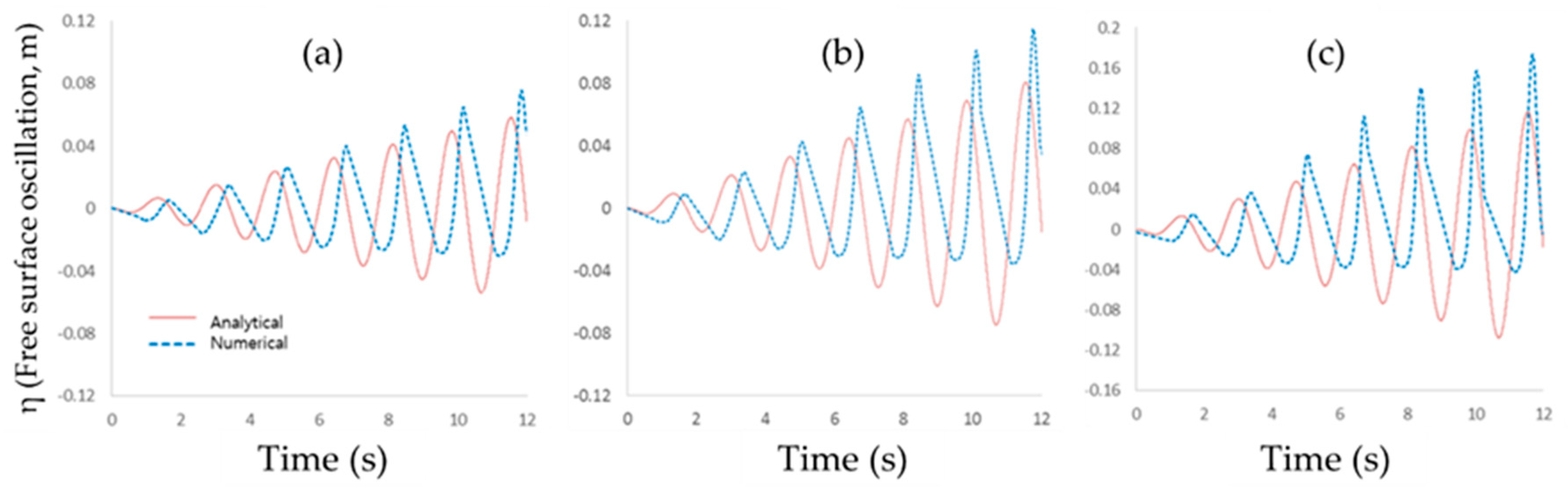
The analytical approach based on linear potential theory has been adopted traditionally to predict sloshing flow under excited small amplitudes, and this approach has shown good results for the actual linear sloshing flow [18,19,20]. In this chapter, the analytical solution is used as reference of linear sloshing flow for observing the nonlinearity of present sloshing behavior. A total of three cases (Cases 1, 2 and 3) were considered for observing nonlinearity of sloshing elevations. Figure 3 shows the comparison of sloshing wave elevation between numerical and analytical solutions. It can be observed that the discrepancy of elevations increase gradually due to the nonlinearity of sloshing flow as the Reynolds number increases.

Figure 3a is the result of Case 1 (Re = 1.8 × 10⁴). Although the magnitude of amplitudes between analytical and numerical results matches well initially, the phase difference gradually increases, as time goes by, due to the influence of nonlinearity and wall friction. Therefore, it seems to be that applying the analytical solution to estimate free-surface oscillation is unreasonable even in terms of rough criteria. Figure 3b,c show the results of Case 2 (Re = 2.5 × 10⁴) and Case 3 (Re = 3.6 × 10⁴), respectively. It can be observed that the discrepancy between the local maximum and local minimum values of free-surface elevation increases with time. From the above results, it can be inferred that the sloshing flow (over Re = 1.8 × 10⁴) has a strong nonlinearity and it seems to be very difficult to estimate the sloshing flow using the linear analytical solution.

Skewness analysis is adopted in order to check solution gaps between the analytical and numerical solution. The skewness, S, is defined as follows:

$$S=\frac{E{(x-\epsilon )}^3}{{\sigma }^3}$$

(16)

where the E(z) is the expected value of the quantity z, the ε is mean of the data, and σ is the standard deviation of x. The skewness on the results of Cases 1, 2, and 3 are summarized in

Table 2. The skewness of the numerical results.

Case	S
1	1.111
2	1.567
3	1.759

, and the results indicate a degree of asymmetry on the distribution. The skewness of the linear solution is zero theoretically. Thus, only numerical data were calculated for 12 s in this study. The result shows that the skewness increases from 1.111 to 1.759 and free surface oscillation has a negatively skewed distribution as the Reynolds number increases. It is regarded that an analytical approach cannot give a good solution due to the developing nonlinearity of sloshing.

3.2. Sloshing Characteristics with Reynolds Number Variation

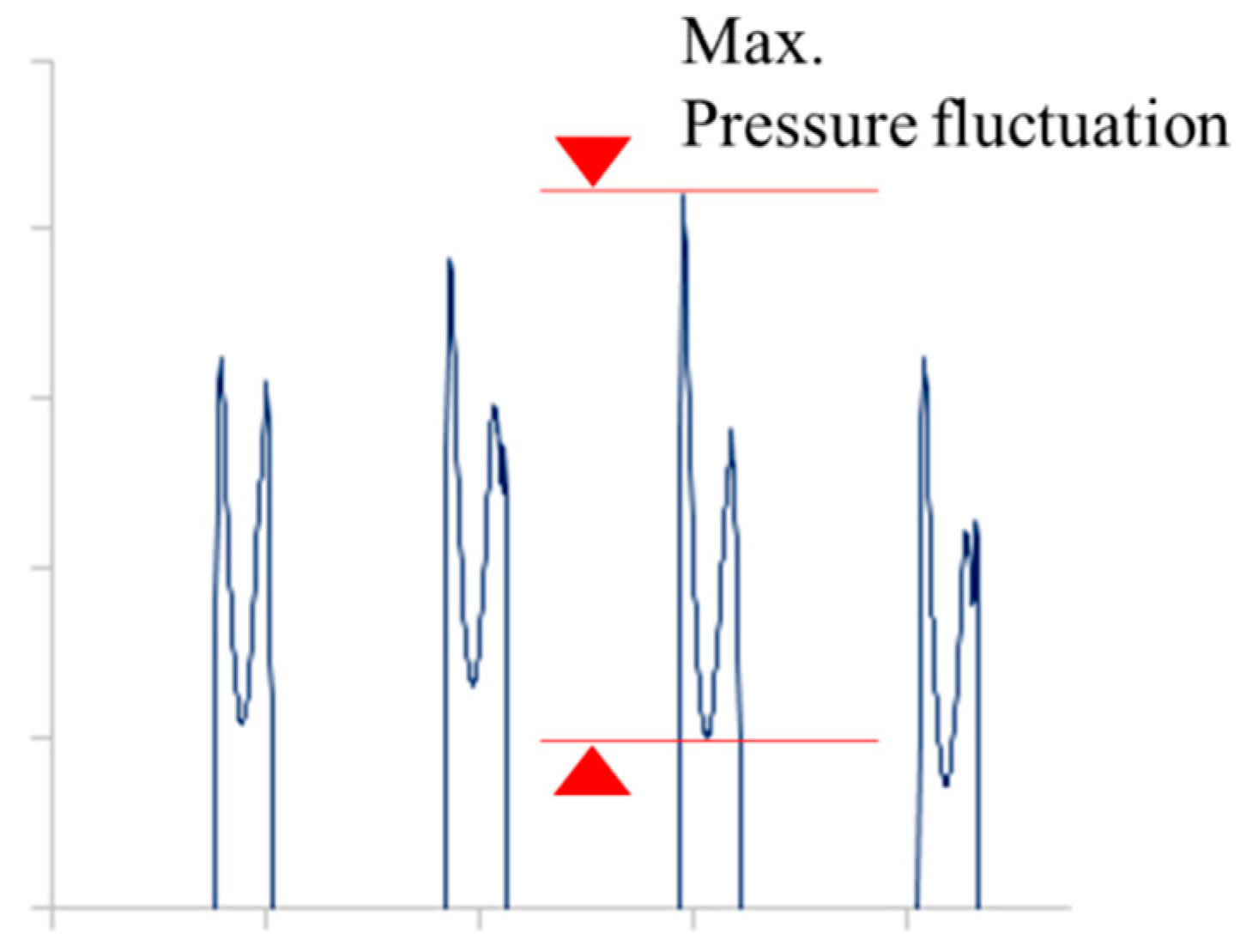
In this work, the characteristics of the pressures of sloshing, which have high Reynolds numbers, are analyzed using the time histories of pressure and fluctuation of peak pressures in sloshing periods. Figure 4 shows the description of pressure fluctuation when the maximum peak pressure occurs.

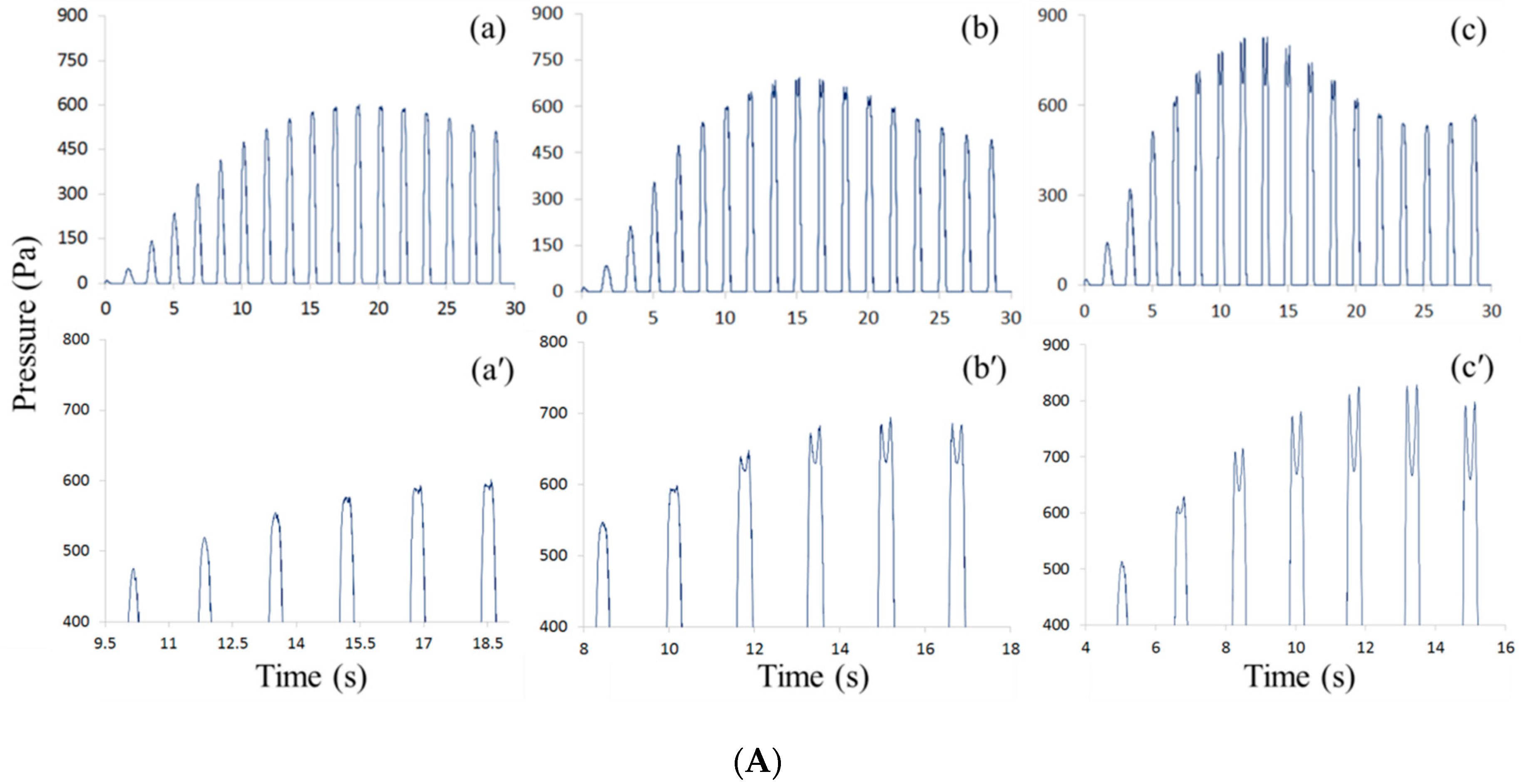
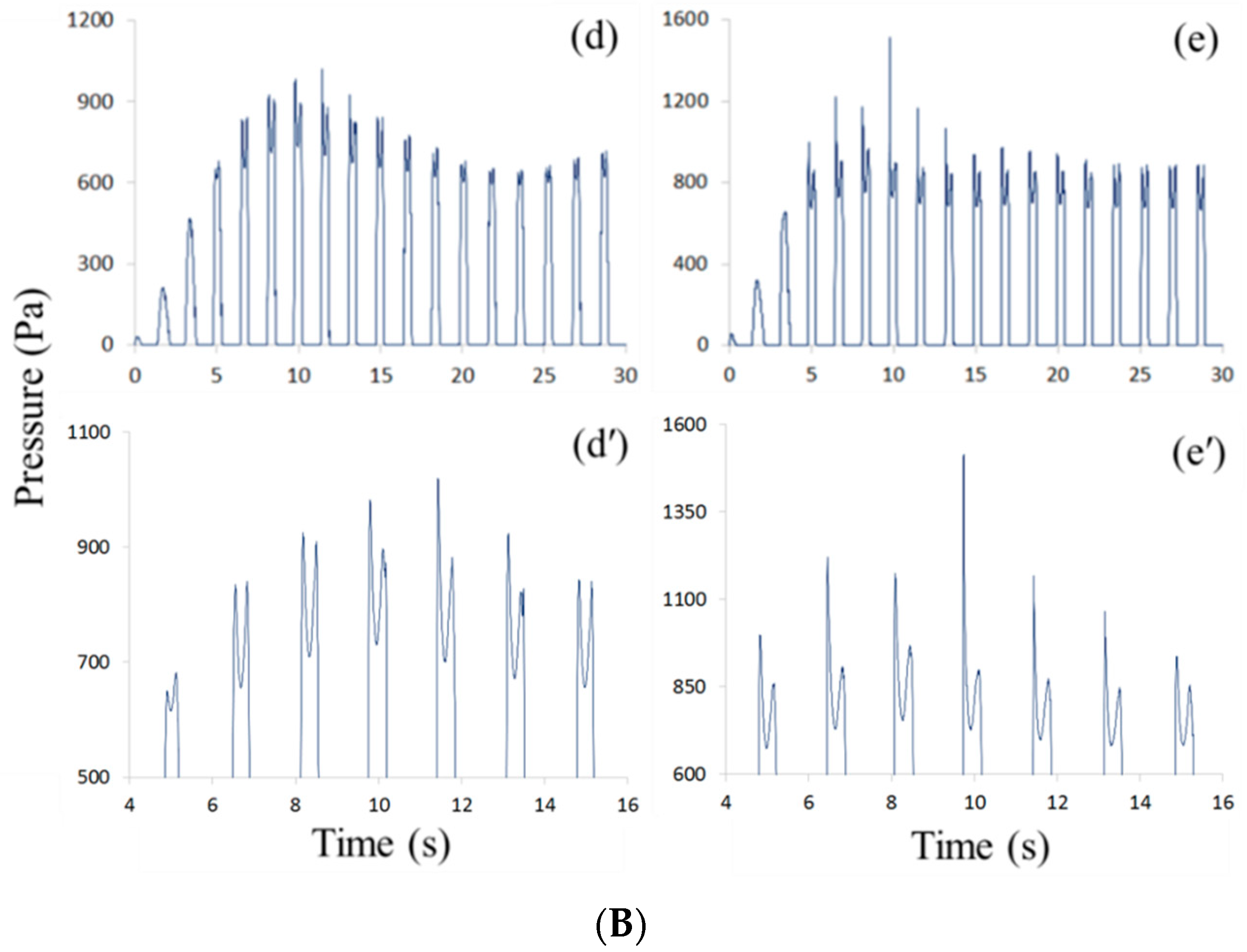
Figure 5A,B show the calculated pressure data at the measuring point and images (a) to (e) indicate the time histories of pressure from 0 to 30 s. Also, images (a’) to (e’) show the enlarged figures near maximum pressure fluctuation for observing the pressure fluctuation of sloshing. Figure 5A shows the time histories of sloshing pressures in Cases 1, 2, and 3. Similarly, Figure 5B indicates the results of Cases 4 and 5. The fluctuation phenomena of the sloshing pressure occur in all of the cases and it can be seen that the fluctuation also increases as the Reynolds number increases. The results of maximum pressure fluctuations of the peak pressure for each case are shown in

Table 3. Maximum pressure fluctuation of peak pressure in each case.

Case	Max. Pressure Fluctuation
No.	Pa
1 (Re 1.8 × 104)	15
2 (Re 2.5 × 104)	64
3 (Re 3.6 × 104)	162
4 (Re 5.0 × 104)	315
5 (Re 7.2 × 104)	789

. It can be seen that the magnitude of fluctuation gradually increases from 15 Pa to 789 Pa.

In Figure 5A, It was found that the pressure fluctuation phenomena start to show at the seventh sloshing pressure cycle in Case 1 and at the sixth and fourth sloshing pressure cycles in Cases 2 and 3, respectively. Figure 5B shows the fluctuation of the peak pressure starts from the fourth pressure cycle, in spite of the increase of the Reynolds number. This means that at least four or more cycles of developmental time are required until characteristics of the nonlinear sloshing flow become manifest. In addition, in the result of Case 5, (e) and (e’), large pressure fluctuation occurs near 9.7 s within 0.1 s, which can be considered an impact pressure. When the impact pressure is generated, a pressure difference of 789 Pa is generated. It is about 48% of the peak pressure.

The reason for the occurrence of the fluctuations is because the kinetic energy of the sloshing by the periodic exciting forces, which were superposed gradually with time, lead to nonlinearity. It seems that, as a result, the fluctuation phenomena appear due to the instability of the wave crest, which occurs due to the increased nonlinearity.

3.3. Comparison of Sloshing Characteristics by FFT Analysis

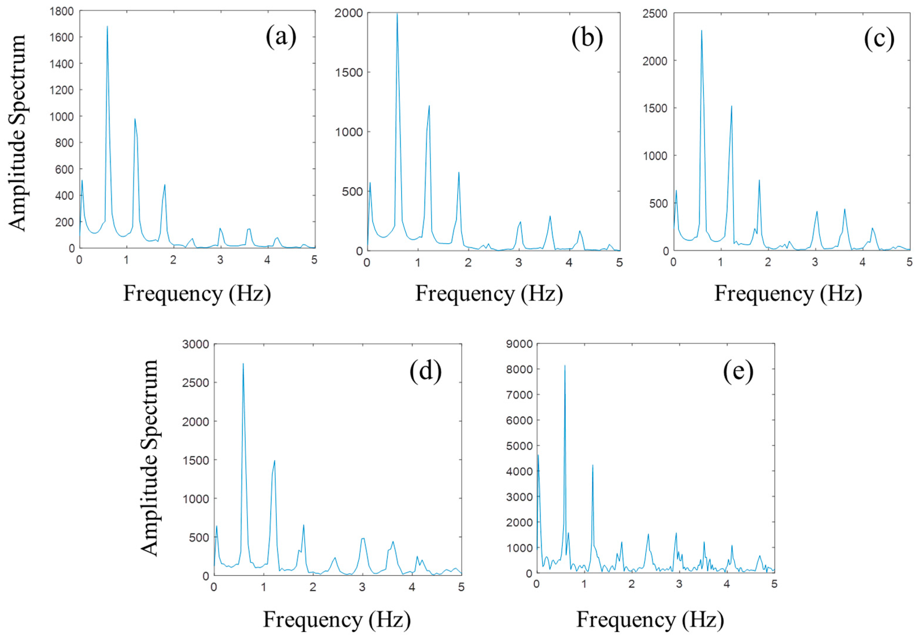
The FFT analysis was performed using the time series data of sloshing pressures obtained from the numerical analysis from 0 to 30 s, and the results are shown in Figure 6. High frequency noise over 5 Hz was observed in all results and the FFT algorithm with a cut off of 5 Hz was used to filter the high frequency noise. It is shown that the peaks of the amplitude spectrum exactly coincided with 0.586 Hz, which is the excited frequency of the fluid motion, and the frequencies corresponding to integral multiples of the excitation frequency have a dominant influence on the sloshing flow. It can be seen that as the Reynolds number increases, the maximum magnitude of the amplitude spectrum increases proportionally. For a more quantitative analysis, the magnitude of the sloshing peak pressure, moments of maximum peak pressure in the periods of sloshing, and maximum amplitude spectrum are summarized in

Table 4. Maximum peak pressure and amplitude spectrum in each case.

Case	PMax		Max. Amplitude Spectrum
No.	Pa	Second	-
1 (Re 1.8 × 104)	602	18.5	1682
2 (Re 2.5 × 104)	695	15.1	1994
3 (Re 3.6 × 104)	829	11.7	2317
4 (Re 5.0 × 104)	1020	11.4	2748
5 (Re 7.2 × 104)	1520	9.7	3430

. Table 4 shows that the maximum pressure and the amplitude spectrum increase as the Reynolds number increases. Especially in Case 5, it is considered that the impact pressure appears to be high by rapid pressure changes as a result of the violent sloshing phenomena.

In Figure 6, saw-toothed amplitude spectra are observed in Cases 3 to 5 at around 1.758 Hz, which is three times the excited frequency. It can be explained that the nonlinear characteristics such as irregular wave crests and breaking waves are related to these phenomena. The saw-toothed amplitude spectrum appears frequently with the increase of the Reynolds number. In Case 5, which has fully developed nonlinearity of sloshing, the saw-toothed amplitude spectra occur at entire integrals of the excitation frequency. It seems that the influence of an excitation frequency attenuates in high frequency regions.

This comparison study by FFT analysis shows that both amplitude spectrum and peak pressure analysis seem to be reasonable in order to understand the sloshing pressure characteristics. However, it is considered that the FFT analysis is more useful in the quantitative analysis when the sloshing phenomena become violent and sloshing pressure is appearing in greater complexity.

3.4. Visual Observation on the Sloshing Impact Motion

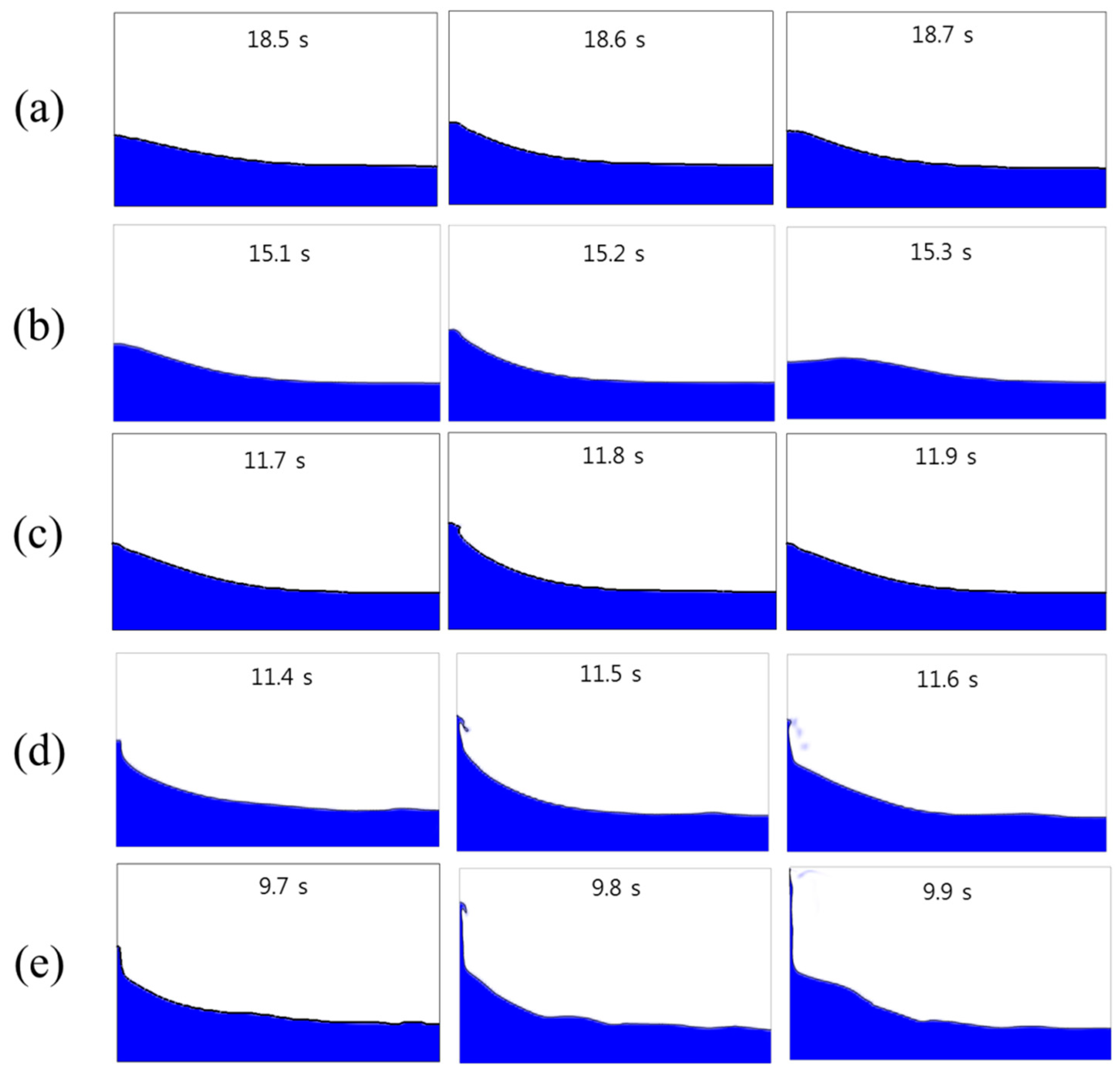
The visualized results as shown in Figure 7 represent the characteristics of a typical first order sloshing flow for a total of 0.3 s with 0.1 s intervals after obtaining peak pressures. Images (a) to (e) denote the results of Cases 1 to 5, respectively. In Figure 7a, it can be observed that the elliptical shape of the wave crest appears at 18.6 s, and Figure 7b shows clearly a larger elliptical wave shape than Case 1 at 15.2 s, after the maximum pressure appears. This local nonlinear flow of wave crest seems to cause fluctuations of peak pressure and the irregular shape of wave crest is observed from Figure 7c. In case of Figure 7d, the wave breaking phenomena can be observed clearly from 11.5 s. This means that the violent sloshing appears from the Reynolds number of 5.0 × 10⁴. The typical characteristics of violent sloshing such as overturning and breaking waves can be observed. In Figure 7e, it seems to be that the more violent sloshing flow appears due to the superposed strong nonlinear fluid flow, with the increases of the Reynolds number. Overall, the wave elevation increases in proportion to the Reynolds numbers, and also the sloshing flows in each case show developing irregular flow patterns as the Reynolds number increases.

4. Conclusions

The sloshing phenomena in the rectangular tank have been numerically analyzed using the VOF method, and the characteristics of sloshing pressures were investigated for various Reynolds number flow. The time series results of the sloshing pressures were analyzed by FFT algorithm, and the magnitude of the amplitude spectrum was compared.

As a result, the reason for the occurrence of the pressure fluctuations was because the kinetic energy of the sloshing by the periodic exciting forces, which was superposed gradually with time, led to nonlinearity and the fluctuation phenomena appeared due to the instability of wave crest, which occurred due to the increased nonlinearity. It is confirmed that overall results show characteristics of first order of sloshing resonance flow, and the frequencies corresponding to integral multiples of excited frequency (0.586 Hz) have a dominant influence on the sloshing flow.

The saw-toothed amplitude spectra were observed in Cases 3 to 5 around 1.758 Hz, which is three times the excited frequency. The nonlinear characteristics such as irregular crests and breaking waves were related to these phenomena. The saw-toothed amplitude spectrum appeared frequently with the increase of Reynolds number.

The flow patterns near the measuring point, changing from the elliptical shape to the irregular shape, are induced by the nonlinear oscillation as the Reynolds number increases. This study provides useful information as a reference for industries that require specific sloshing phenomena analysis.

References

- Xue, M.-A.; Lin, P. Numerical study of ring baffle effects on reducing violent liquid sloshing. Comput. Fluids 2011, 52, 116–129. [Google Scholar] [CrossRef]
- Wang, W.; Guo, Z.; Peng, Y.; Zhang, Q. A numerical study of the effects of the T-shaped baffles on liquid sloshing in horizontal elliptical tanks. Ocean Eng. 2016, 111, 543–568. [Google Scholar] [CrossRef]
- Liu, D.; Tang, W.; Wang, J.; Xue, H.; Wang, K. Comparison of laminar model, RANS, LES and VLES for simulation of liquid sloshing. Appl. Ocean Res. 2016, 59, 638–649. [Google Scholar] [CrossRef]
- Godderidge, B. A Phenomenological Rapid Sloshing Model for Use as an Operator Guidance System on Liquefied Natural Gas Carriers. Doctoral Dissertation, University of Southampton, Southampton, UK, 2009. [Google Scholar]
- Kim, Y. Numerical simulation of sloshing flows with impact load. Appl. Ocean Res. 2001, 23, 53–62. [Google Scholar] [CrossRef]
- Chen, B.-F.; Nokes, R. Time-independent finite difference analysis of fully non-linear and viscous fluid sloshing in a rectangular tank. J. Comput. Phys. 2005, 209, 47–81. [Google Scholar] [CrossRef]
- Wu, C.-H.; Chen, B.-F.; Hung, T.-K. Hydrodynamic forces induced by transient sloshing in a 3D rectangular tank due to oblique horizontal excitation. Comput. Math. Appl. 2013, 65, 1163–1186. [Google Scholar] [CrossRef]
- Arafa, M. Finite element analysis of sloshing in rectangular liquid-filled tanks. J. Vib. Control 2007, 13, 883–903. [Google Scholar] [CrossRef]
- Mitra, S.; Upadhyay, P.P.; Sinhamahapatra, K.P. Slosh dynamics of inviscid fluids in two-dimensional tanks of various geometry using finite element method. Int. J. Numer. Methods Fluids 2008, 56, 1625–1651. [Google Scholar] [CrossRef]
- Nayak, S.K.; Biswal, K.C. Quantification of seismic response of partially filled rectangular liquid tank with submerged block. J. Earthq. Eng. 2013, 17, 1023–1062. [Google Scholar] [CrossRef]
- Chen, Y.G.; Djidjeli, K.; Price, W.G. Numerical simulation of liquid sloshing phenomena in partially filled containers. Comput. Fluids 2009, 38, 830–842. [Google Scholar] [CrossRef]
- Akyildız, H.; Ünal, N.E. Sloshing in a three-dimensional rectangular tank: Numerical simulation and experimental validation. Ocean Eng. 2006, 33, 2135–2149. [Google Scholar] [CrossRef]
- Li, J.G.; Hamamoto, Y.; Liu, Y.; Zhang, X. Sloshing impact simulation with material point method and its experimental validations. Comput. Fluids 2014, 103, 86–99. [Google Scholar] [CrossRef]
- Birknes-Berg, J.; Pedersen, G.K. The “Chain of Markers” Code Applied to Large Scale Problems; Solitary Waves, Sloshing and a Plunging Wave. Research Report in Mechanics. 2017. Available online: http://urn.nb.no/URN:NBN:no-23419 (accessed on 1 September 2017).
- Fox, D.W.; Kuttler, J.R. Sloshing frequencies, Zeitschrift für Angewandte Mathematik und Physik (ZAMP). J. Appl. Math. Phys. 1983, 34, 668–696. [Google Scholar]
- Lee, D.; Kim, M.H.; Kwon, S.H.; Kim, J.W.; Lee, Y.B. A parametric sensitivity study on LNG tank sloshing loads by numerical simulations. Ocean Eng. 2007, 34, 3–9. [Google Scholar] [CrossRef]
- Godderidge, B.; Turnock, S.; Tan, M.; Earl, C. An investigation of multiphase CFD modelling of a lateral sloshing tank. Comput. Fluids 2009, 38, 183–193. [Google Scholar] [CrossRef]
- Faltinsen, O.M. A numerical nonlinear method of sloshing in tanks with two-dimensional flow. J. Ship Res. 1978, 22, 193–202. [Google Scholar]
- Liu, D.; Lin, P. A numerical study of three-dimensional liquid sloshing in tanks. J. Comput. Phys. 2008, 227, 3921–3939. [Google Scholar] [CrossRef]
- Frandsen, J.B. Sloshing motions in excited tanks. J. Comput. Phys. 2004, 196, 53–87. [Google Scholar] [CrossRef]
- Parthasarathty, N.; Kim, H.; Choi, Y.H.; Lee, Y.W. A numerical study on sloshing impact loads in prismatic tanks under forced horizontal motion. J. Korean Soc. Mar. Eng. 2017, 41, 150–155. [Google Scholar] [CrossRef]
- Kim, H.; Choi, Y.-H.; Lee, Y.-W. Numerical analysis of sloshing impact in horizontally excited prismatic tanks. Prog. Comput. Fluid Dyn. 2017, 17, 361–367. [Google Scholar] [CrossRef]
- Kishev, Z.R.; Hu, C.; Kashiwagi, M. Numerical simulation of violent sloshing by a CIP-based method. J. Mar. Sci. Technol. 2006, 11, 111–122. [Google Scholar] [CrossRef]
Figure 1.
Schematic diagram of a 2D rectangular tank and mesh generation.
Figure 2.
Comparison between numerical and experimental data [23].
Figure 3.
Comparison of sloshing wave elevation between numerical and analytical solutions; (a) Case 1; (b) Case 2; and (c) Case 3.
Figure 4.
Description of the maximum pressure fluctuation of peak pressure.
Figure 5.
(A) Pressure patterns of slosh for Case 1 (a,a′), Case 2 (b,b′) and Case 3 (c,c′); (a,b,c) are time histories of pressures from 0 to 30 s at MP for each cases; (a′,b′,c′) are the enlarged figures near the maximum pressures. (B) Pressure patterns of slosh for Case 4 (d,d′) and Case 5 (e,e′); (d,e) are time histories of pressures from 0 to 30 s at MP for each cases; (d′,e′) are the enlarged figures near the maximum pressures.
Figure 6.
FFT analysis of the time historical data of the sloshing pressure; (a) Case 1, (b) Case 2, (c) Case 3, (d) Case 4, and (e) Case 5.
Figure 7.
Visualization of sloshing flows in the rectangular tank at impact moments of each case; (a) Case 1, (b) Case 2, (c) Case 3, (d) Case 4, and (e) Case 5.