Microwave Imaging System Based on Signal Analysis in a Planar Environment for Detection of Abdominal Aortic Aneurysms

 ,
,  ,
,  ,
,  , , and
Abstract
:1. Introduction
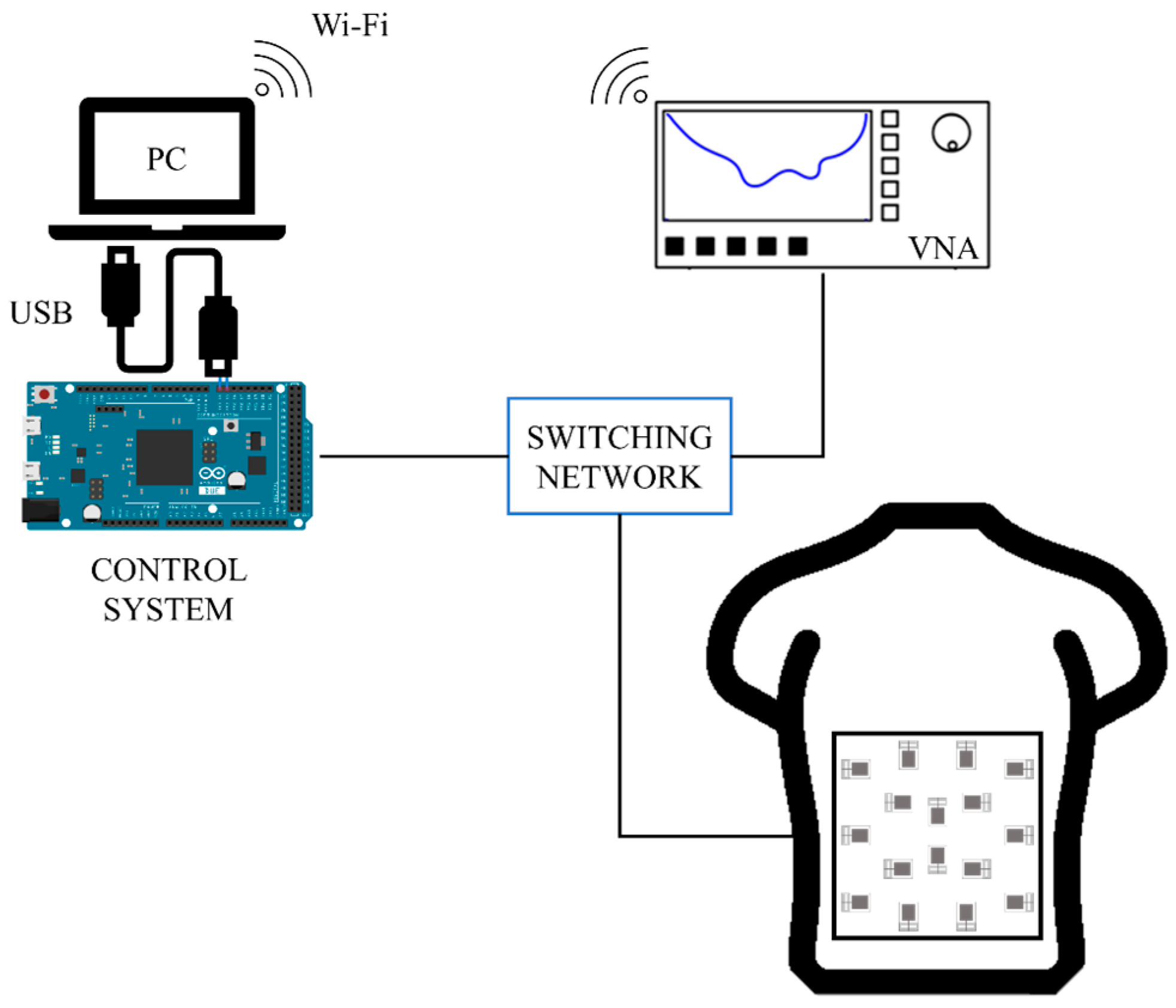
2. Hardware System
2.1. Antennas
2.2. Switching and Electronic Control System
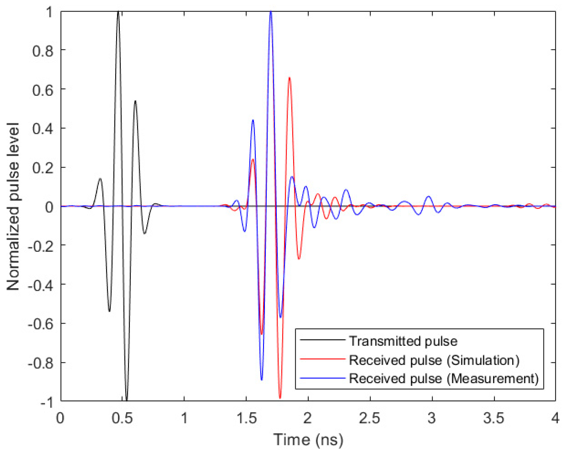
3. Image Generation and Processing
4. Calibration and Fine-Tuning
4.1. Calibration of Measurements at Planes Parallel to the Antennas
4.2. Calibration of Measurements at Different Positions within a Plane
5. Experimental Validation and Proof-of-Concept
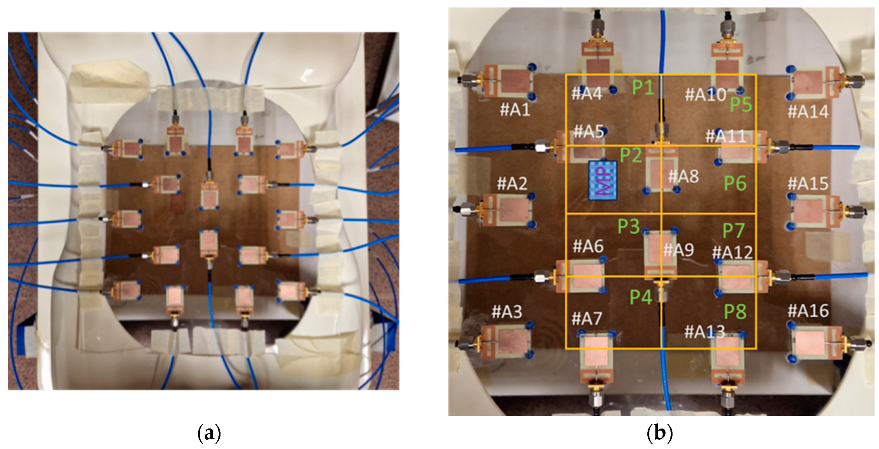
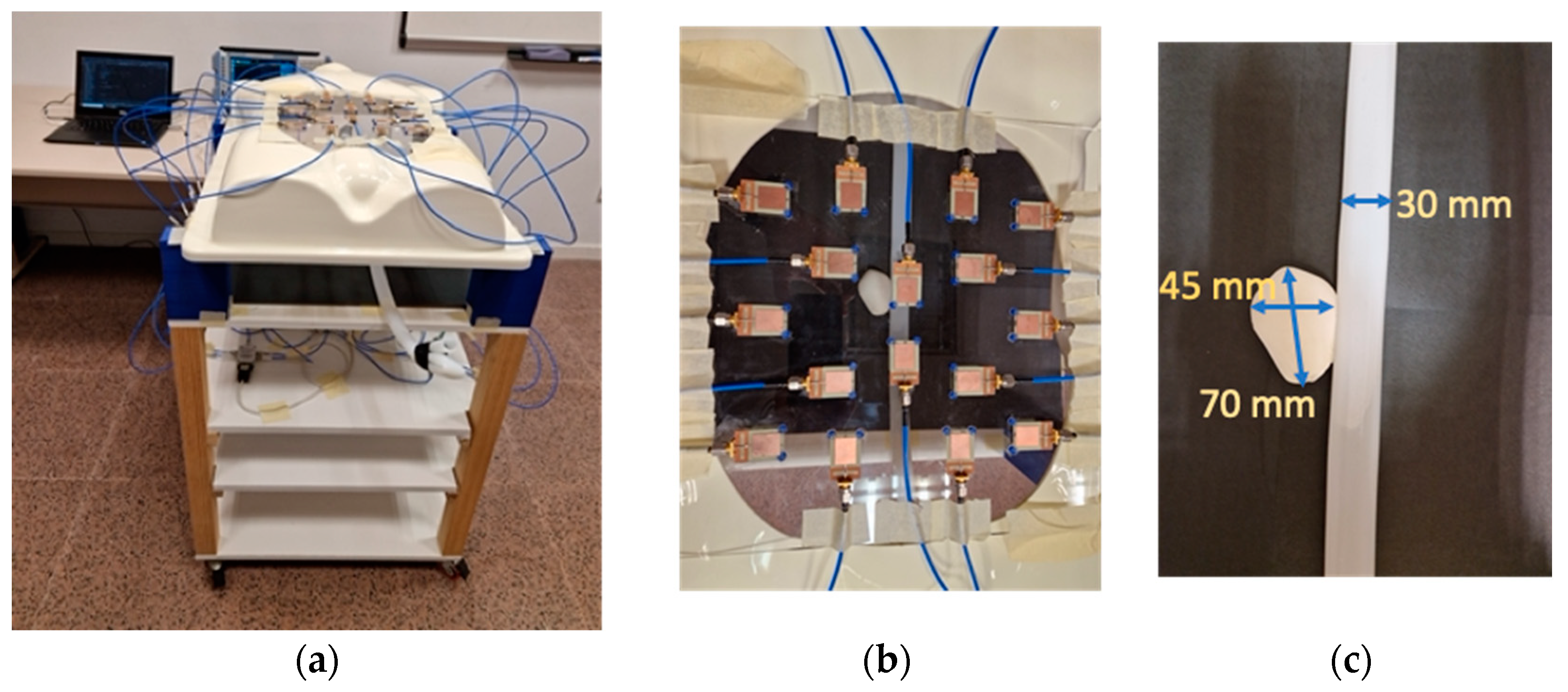
5.1. Experimental Setup
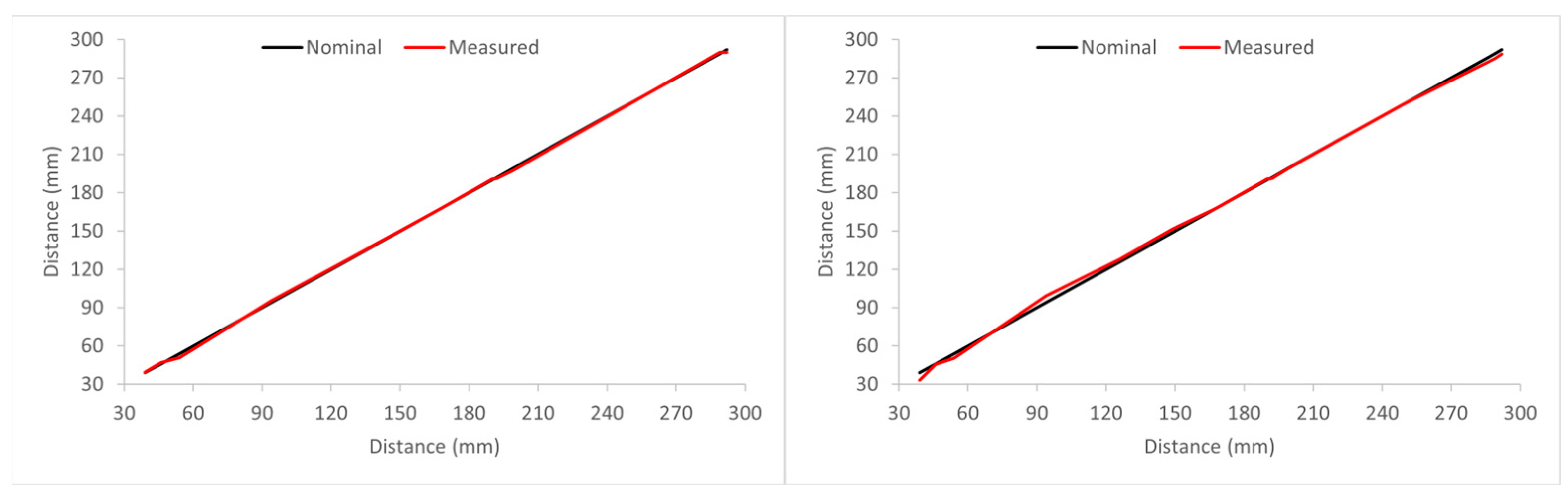
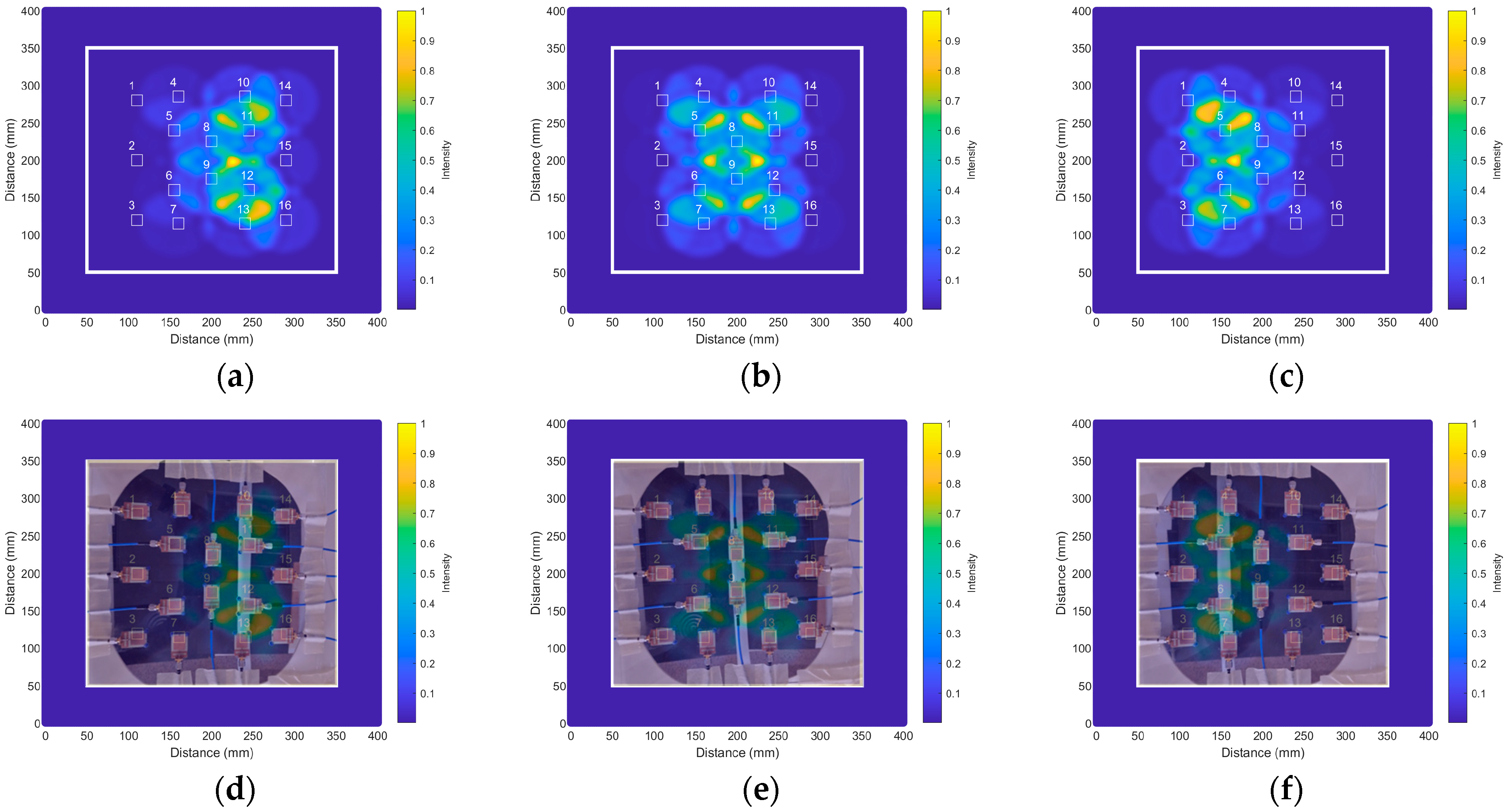
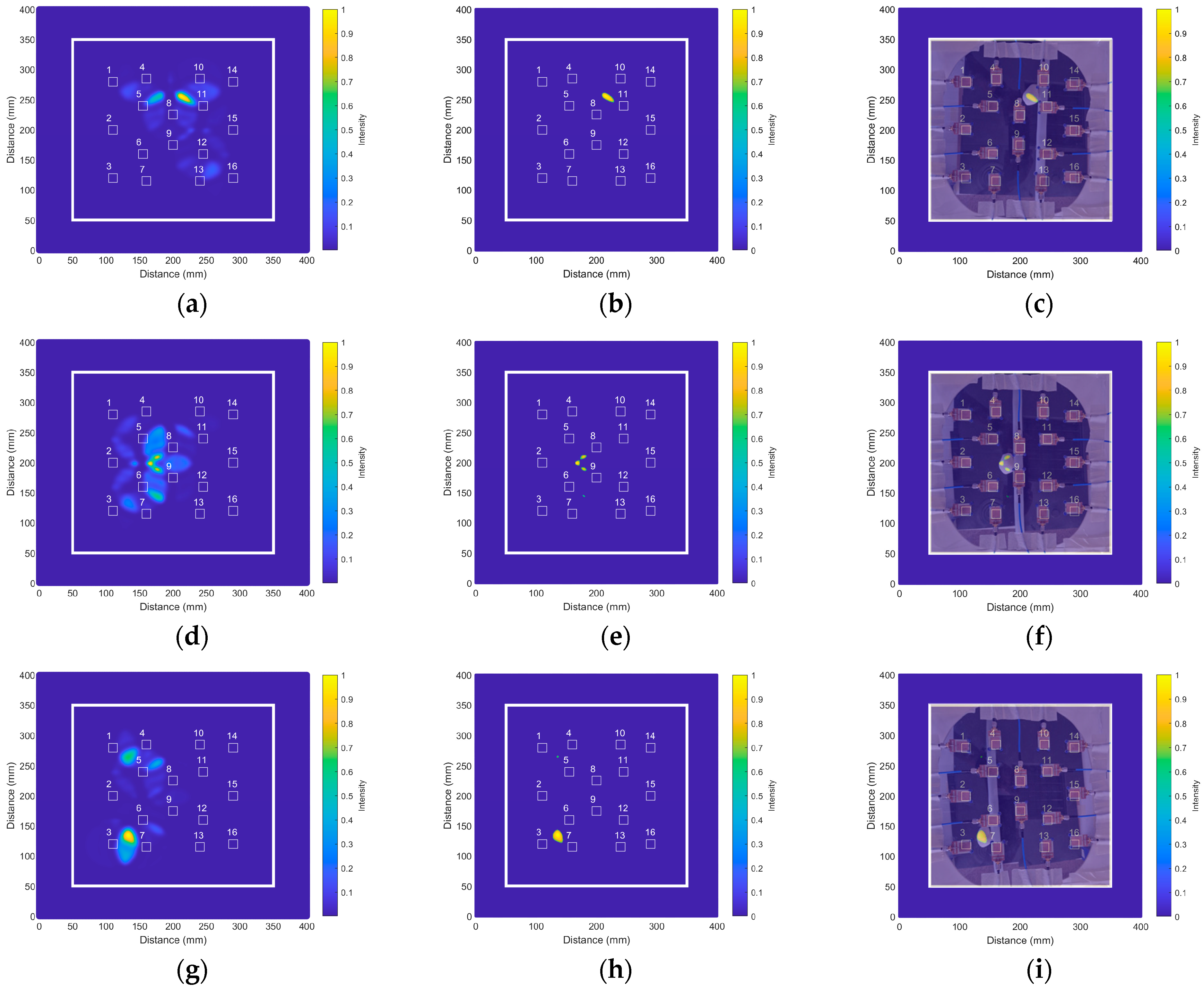
5.2. Proof-of-Concept
6. Conclusions
Author Contributions
Funding
Institutional Review Board Statement
Informed Consent Statement
Data Availability Statement
Conflicts of Interest
References
- Sakalihasan, N.; Limet, R.; Defawe, O.D. Abdominal aortic aneurysm. Lancet 2005, 365, 1577–1589. [Google Scholar] [CrossRef]
- Perrin, M. Venous aneurysms. Phlebolymphology 2006, 13, 172–176. [Google Scholar]
- Gillespie, D.L.; Villavicencio, J.L.; Gallagher, C.; Chang, A.; Hamelink, J.K.; Fiala, L.A.; O’Donnell, S.D.; Jackson, M.R.; Pikoulis, E.; Rich, N.M. Presentation and management of venous aneurysms. J. Vasc. Surg. 1997, 26, 845–852. [Google Scholar] [CrossRef] [PubMed]
- Irwin, C.; Synn, A.; Kraiss, L.; Zhang, Q.; Griffen, M.M.; Hunter, G.C. Metalloproteinase expression in venous aneurysms. J. Vasc. Surg. 2008, 48, 1278–1285. [Google Scholar] [CrossRef] [PubMed]
- Kumar, Y.; Hooda, K.; Li, S.; Goyal, P.; Gupta, N.; Adeb, M. Abdominal aortic aneurysm: Pictorial review of common appearances and complication. Ann. Transl. Med. 2017, 5, 256. [Google Scholar] [CrossRef] [PubMed]
- Hong, H.; Yang, Y.; Liu, B.; Cai, W. Imaging of abdominal aortic aneurysm: The present and the future. Curr. Vasc. Pharmacol. 2010, 8, 808–819. [Google Scholar] [CrossRef]
- Jacob, A.D.; Barkley, P.L.; Broadbent, K.C.; Huynh, T.T.T. Abdominal aortic aneurysm screening. Semin. Roentgenol. 2015, 50, 118–126. [Google Scholar] [CrossRef] [PubMed]
- Wang, X.; Ghayesh, M.H.; Kotousov, A.; Zander, A.C.; Psaltis, P.J. Dynamical Influences of Different Aneurysm Sizes on Rupture Risk of Abdominal Aorta. In Proceedings of the 1st International Conference on Mechanical System Dynamics (ICMSD 2022), Nanjing, China, 24–27 August 2022; pp. 33–38. [Google Scholar] [CrossRef]
- Anagnostakos, J.; Lal, B.K. Abdominal aortic aneurysms. Prog. Cardiovasc. Dis. 2021, 65, 34–43. [Google Scholar] [CrossRef] [PubMed]
- Hoskins, P.; Semple, S.; White, P.; Richards, J. Imaging of aneurysms. In Biomechanics and Mechanobiology of Aneurysms. Studies in Mechanobiology, Tissue Engineering and Biomaterials; McGloughlin, T., Ed.; Springer: Berlin/Heidelberg, Germany, 2011; Volume 7, pp. 35–65. [Google Scholar] [CrossRef]
- de Hoop, H.; Petterson, N.J.; van de Vosse, F.N.; van Sambeek, M.R.H.M.; Schwab, H.-M.; Lopata, R.G.P. Multiperspective ultrasound strain imaging of the abdominal aorta. IEEE Trans. Med. Imaging 2020, 39, 3714–3724. [Google Scholar] [CrossRef]
- Moradi, S.; Ferdinando, H.; Zienkiewicz, A.; Särestöniemi, M.; Myllylä, T. Measurement of cerebral circulation in human. In Cerebral Circulation—Updates on Models, Diagnostics and Treatments of Related Diseases; Scerrati, A., Ricciardi, L., Dones, F., Eds.; IntechOpen: London, UK, 2022. [Google Scholar] [CrossRef]
- Martínez-Lozano, A.; Blanco-Angulo, C.; García-Martínez, H.; Gutiérrez-Mazón, R.; Torregrosa-Penalva, G.; Ávila-Navarro, E.; Sabater-Navarro, J.M. UWB-printed rectangular-based monopole antenna for biological tissue analysis. Electronics 2021, 10, 304. [Google Scholar] [CrossRef]
- Shao, W.; McCollough, T. Advances in microwave near-field imaging. IEEE Microw. Mag. 2020, 21, 94–119. [Google Scholar] [CrossRef]
- Ketavath, K.N.; Gopi, D.; Rani, S.S. In-vitro test of miniaturized CPW-fed implantable conformal patch antenna at ISM band for biomedical applications. IEEE Access 2019, 7, 43547–43554. [Google Scholar] [CrossRef]
- Kiani, S.; Rezaei, P.; Fakhr, M. A CPW-fed wearable antenna at ISM band for biomedical and WBAN applications. Wirel. Netw. 2021, 27, 735–745. [Google Scholar] [CrossRef]
- Fear, E.C.; Meaney, P.M.; Stuchly, M.A. Microwaves for breast cancer detection? IEEE Potentials 2003, 22, 12–18. [Google Scholar] [CrossRef]
- Martínez-Lozano, A.; Blanco-Angulo, C.; Rodríguez-Martínez, A.; Juan, C.G.; García-Martínez, H.; Sabater-Navarro, J.M.; Ávila-Navarro, E. Toward intraoperative brain-shift detection through microwave imaging system. IEEE Trans. Instrum. Meas. 2023, 72, 4011411. [Google Scholar] [CrossRef]
- Islam, M.T.; Mahmud, M.Z.; Islam, M.T.; Kibria, S.; Samsuzzaman, S. A low cost and portable microwave imaging system for breast tumor detection using UWB directional antenna array. Sci. Rep. 2019, 9, 15491. [Google Scholar] [CrossRef] [PubMed]
- Blanco-Angulo, C.; Martínez-Lozano, A.; Gutiérrez-Mazón, R.; Juan, C.G.; García-Martínez, H.; Arias-Rodríguez, J.; Sabater-Navarro, J.M.; Ávila-Navarro, E. Non-invasive microwave-based imaging system for early detection of breast tumours. Biosensors 2022, 12, 752. [Google Scholar] [CrossRef] [PubMed]
- Hamza, M.N.; Abdulkarim, Y.I.; Saeed, S.R.; Altıntaş, O.; Mahmud, R.H.; Appasani, B.; Ravariu, C. Low-cost antenna-array-based metamaterials for non-invasive early-stage breast tumor detection in the human body. Biosensors 2022, 12, 828. [Google Scholar] [CrossRef]
- Lauteslager, T.; Tømmer, M.; Lande, T.S.; Constandinou, T.G. Dynamic microwave imaging of the cardiovascular system using ultra-wideband radar-on-chip devices. IEEE Trans. Biomed. Eng. 2022, 69, 2935–2946. [Google Scholar] [CrossRef] [PubMed]
- Hossain, A.; Islam, M.T.; Rahman, T.; Chowdhury, M.E.H.; Tahir, A.; Kiranyaz, S.; Mat, K.; Beng, G.K.; Soliman, M.S. Brain tumor segmentation and classification from sensor-based portable microwave brain imaging system using lightweight deep learning models. Biosensors 2023, 13, 302. [Google Scholar] [CrossRef]
- Persson, M.; Fhager, A.; Trefná, H.D.; Yu, Y.; McKelvey, T.; Pegenius, G.; Karlsson, J.-E.; Elam, M. Microwave-based stroke diagnosis making global prehospital thrombolytic treatment possible. IEEE Trans. Biomed. Eng. 2014, 61, 2806–2817. [Google Scholar] [CrossRef] [PubMed]
- Tobon Vasquez, J.A.; Scapaticci, R.; Turvani, G.; Bellizzi, G.; Rodriguez-Duarte, D.O.; Joachimowicz, N.; Duchêne, B.; Tedeschi, E.; Casu, M.R.; Crocco, L.; et al. A prototype microwave system for 3D brain stroke imaging. Sensors 2020, 20, 2607. [Google Scholar] [CrossRef] [PubMed]
- Moloney, B.M.; O’Loughlin, D.; Abd Elwahab, S.; Kerin, M.J. Breast cancer detection—A synopsis of conventional modalities and the potential role of microwave imaging. Diagnostics 2020, 10, 103. [Google Scholar] [CrossRef] [PubMed]
- Nikolova, N.K. Microwave imaging for breast cancer. IEEE Microw. Mag. 2011, 12, 78–94. [Google Scholar] [CrossRef]
- Sohani, B.; Khalesi, B.; Ghavami, N.; Ghavami, M.; Dudley, S.; Rahmani, A.; Tiberi, G. Detection of haemorrhagic stroke in simulation and realistic 3-D human head phantom using microwave imaging. Biomed. Signal Process. Control 2020, 61, 102001. [Google Scholar] [CrossRef]
- Preece, A.W.; Craddock, I.; Shere, M.; Jones, L.; Winton, H.L. MARIA M4: Clinical evaluation of a prototype ultrawideband radar scanner for breast cancer detection. J. Med. Imaging 2016, 3, 033502. [Google Scholar] [CrossRef]
- Massey, H.; Ridley, N.; Lyburn, I. Radiowave detection of breast cancer in the symptomatic clinic—A multi-centre study. In Proceedings of the International Cambridge Conference on Breast Imaging, Cambridge, UK, 3–4 July 2017. [Google Scholar]
- Janjic, A.; Cayoren, M.; Akduman, I.; Yilmaz, T.; Onemli, E.; Bugdayci, O.; Aribal, M.E. SAFE: A novel microwave imaging system design for breast cancer screening and early detection—Clinical evaluation. Diagnostics 2021, 11, 533. [Google Scholar] [CrossRef]
- Rodriguez-Duarte, D.O.; Tobon Vasquez, J.A.; Scapaticci, R.; Turvani, G.; Cavagnaro, M.; Casu, M.R.; Crocco, L.; Vipiana, F. Experimental validation of a microwave system for brain stroke 3-D imaging. Diagnostics 2021, 11, 1232. [Google Scholar] [CrossRef]
- Hampson, M. New Smart Helmet Rapidly Assesses Stroke Patients. IEEE Spectrum. 2021. Available online: https://spectrum.ieee.org/new-smart-helmet-design-rapidly-assesses-stroke-patients (accessed on 3 February 2024).
- Candefjord, S.; Winges, J.; Malik, A.A.; Yu, Y.; Rylander, T.; McKelvey, T.; Fhager, A.; Elam, M.; Persson, M. Microwave technology for detecting traumatic intracranial bleedings: Tests on phantom of subdural hematoma and numerical simulations. Med. Biol. Eng. Comput. 2017, 55, 1177–1188. [Google Scholar] [CrossRef]
- Mobashsher, A.T.; Bialkowski, K.S.; Abbosh, A.M.; Crozier, S. Design and experimental evaluation of a non-invasive microwave head imaging system for intracranial haemorrhage detection. PLoS ONE 2016, 11, e0152351. [Google Scholar] [CrossRef] [PubMed]
- Mobashsher, A.T.; Abbosh, A.M. On-site rapid diagnosis of intracranial hematoma using portable multi-slice microwave imaging system. Sci. Rep. 2016, 6, 37620. [Google Scholar] [CrossRef]
- Mobashsher, A.T.; Mahmoud, A.; Abbosh, A.M. Portable wideband microwave imaging system for intracranial hemorrhage detection using improved back-projection algorithm with model of effective head permittivity. Sci. Rep. 2016, 6, 20459. [Google Scholar] [CrossRef]
- Quintero, G.; Zurcher, J.-F.; Skrivervik, A.K. System Fidelity Factor: A new method for comparing UWB antennas. IEEE Trans. Antennas Propag. 2011, 59, 2502–2512. [Google Scholar] [CrossRef]
- Marinov, O. Noise Partition in S-parameter Measurement. In Proceedings of the 22nd International Conference on Noise and Fluctuations (ICNF), Montpellier, France, 24–28 June 2013. [Google Scholar] [CrossRef]
- Reimer, T.; Solis-Nepote, M.; Pistorius, S. The impact of the inverse chirp z-transform on breast microwave radar image reconstruction. Int. J. Microw. Wirel. Technol. 2020, 12, 848–854. [Google Scholar] [CrossRef]
- Garrett, J.; Fear, E. A new breast phantom with a durable skin layer for microwave breast imaging. IEEE Trans. Antennas Propag. 2015, 63, 1693–1700. [Google Scholar] [CrossRef]
- AlSawaftah, N.; El-Abed, S.; Dhou, S.; Zakaria, A. Microwave imaging for early breast cancer detection: Current state, challenges, and future directions. J. Imaging 2022, 8, 123. [Google Scholar] [CrossRef]
- Conceição, R.C.; Mohr, J.J.; O’Halloran, M. An Introduction to Microwave Imaging for Breast Cancer Detection; Springer International Publishing: Cham, Switzerland, 2016. [Google Scholar] [CrossRef]
- Elahi, M.A.; O’Loughlin, D.; Lavoie, B.R.; Glavin, M.; Jones, E.; Fear, E.C.; O’Halloran, M. Evaluation of image reconstruction algorithms for confocal microwave imaging: Application to patient data. Sensors 2018, 18, 1678. [Google Scholar] [CrossRef]
- Guo, B.; Wang, Y.; Li, J.; Stoica, P.; Wu, R. Microwave imaging via adaptive beamforming methods for breast cancer detection. J. Electromagn. Waves Appl. 2006, 20, 53–63. [Google Scholar] [CrossRef]
- Blanco-Angulo, C.; Martínez-Lozano, A.; Juan, C.G.; Gutiérrez-Mazón, R.; Arias-Rodríguez, J.; Ávila-Navarro, E.; Sabater-Navarro, J.M. Validation of an RF image system for real-time tracking neurosurgical tools. Sensors 2022, 22, 3845. [Google Scholar] [CrossRef] [PubMed]
- Pozar, D.M. The wave equation and basic plane wave solution. In Microwave Engineering, 3rd ed.; John Wiley & Sons: Hoboken, NJ, USA, 2005; Chapter 1.4; p. 18. [Google Scholar]
- Hasgall, P.A.; Di Gennaro, F.; Baumgartner, C.; Neufeld, E.; Lloyd, B.; Gosselin, M.C.; Payne, D.; Klingenböck, A.; Kuster, N. “IT’IS Database for Thermal and Electromagnetic Parameters of Biological Tissues: Version 4.1”, Found. Res. Inf. Technol. Soc. (IT’IS): Zürich, Switzerland, Version 4.1, Tech. Rep., Feb. 2022. Available online: https://itis.swiss/virtual-population/tissue-properties/overview/ (accessed on 3 February 2024).
- Naghibi, A.; Attari, A.R. Near-field radar-based microwave imaging for breast cancer detection: A study on resolution and image quality. IEEE Trans. Antennas Propag. 2021, 69, 1670–1680. [Google Scholar] [CrossRef]


| Parameter | Value | Parameter | Value | Parameter | Value |
|---|---|---|---|---|---|
| Wsub | 20.0 | W2 | 0.3 | LTL | 10.5 |
| Lsub | 30.0 | L2 | 3.5 | Wslot | 2.3 |
| W1 | 14.0 | G | 2.0 | Lslot | 8.1 |
| L1 | 17.4 | WTL | 0.7 |
| AAA Case | Real Position | IDAS Obtained Position | Positioning Error | |||||
|---|---|---|---|---|---|---|---|---|
| Pos. x | Pos. y | Obt. x | Obt. y | Error x | Rel. Error x | Error y | Rel. Error y | |
| 1 | 221.5 | 256.8 | 216.8 | 256.0 | 4.7 | 2.1% | 0.8 | 0.3% |
| 2 | 213.7 | 184.0 | 227.8 | 197.3 | 14.1 | 6.6% | 13.3 | 7.2% |
| 3 | 216.8 | 140.0 | 218.4 | 143.2 | 1.6 | 0.7% | 3.2 | 2.3% |
| 4 | 173.2 | 264.6 | 177.7 | 253.6 | 4.5 | 2.6% | 11.0 | 4.2% |
| 5 | 180.8 | 201.2 | 172.2 | 199.6 | 8.6 | 4.8% | 1.6 | 0.8% |
| 6 | 176.1 | 137.1 | 180.8 | 143.2 | 4.7 | 2.7% | 6.1 | 4.4% |
| 7 | 140.9 | 259.1 | 136.1 | 261.4 | 4.8 | 3.4% | 2.3 | 0.9% |
| 8 | 137.0 | 185.5 | 133.1 | 180.8 | 3.9 | 2.8% | 4.7 | 2.5% |
| 9 | 140.1 | 135.9 | 136.2 | 134.6 | 3.9 | 2.8% | 1.3 | 1.0% |
Disclaimer/Publisher’s Note: The statements, opinions and data contained in all publications are solely those of the individual author(s) and contributor(s) and not of MDPI and/or the editor(s). MDPI and/or the editor(s) disclaim responsibility for any injury to people or property resulting from any ideas, methods, instructions or products referred to in the content. |
© 2024 by the authors. Licensee MDPI, Basel, Switzerland. This article is an open access article distributed under the terms and conditions of the Creative Commons Attribution (CC BY) license (https://creativecommons.org/licenses/by/4.0/).
Share and Cite
Martínez-Lozano, A.; Gutierrez, R.; Juan, C.G.; Blanco-Angulo, C.; García-Martínez, H.; Torregrosa, G.; Sabater-Navarro, J.M.; Ávila-Navarro, E. Microwave Imaging System Based on Signal Analysis in a Planar Environment for Detection of Abdominal Aortic Aneurysms. Biosensors 2024, 14, 149. https://doi.org/10.3390/bios14030149
Martínez-Lozano A, Gutierrez R, Juan CG, Blanco-Angulo C, García-Martínez H, Torregrosa G, Sabater-Navarro JM, Ávila-Navarro E. Microwave Imaging System Based on Signal Analysis in a Planar Environment for Detection of Abdominal Aortic Aneurysms. Biosensors. 2024; 14(3):149. https://doi.org/10.3390/bios14030149
Chicago/Turabian StyleMartínez-Lozano, Andrea, Roberto Gutierrez, Carlos G. Juan, Carolina Blanco-Angulo, Héctor García-Martínez, Germán Torregrosa, José María Sabater-Navarro, and Ernesto Ávila-Navarro. 2024. "Microwave Imaging System Based on Signal Analysis in a Planar Environment for Detection of Abdominal Aortic Aneurysms" Biosensors 14, no. 3: 149. https://doi.org/10.3390/bios14030149