Adhesion of Soft Materials to Rough Surfaces: Experimental Studies, Statistical Analysis and Modelling

Abstract

Adhesion between rough surfaces is an active field of research where both experimental studies and theoretical modelling are used. However, it is rather difficult to conduct precise experimental evaluations of adhesive properties of the so-called anti-adhesive materials. Hence, it was suggested earlier by Purtov et al. (2013) to prepare epoxy resin replicas of surfaces having different topography and conduct depth-sensing indentation of the samples using a micro-force tester with a spherical smooth probe made of the compliant polydimethylsiloxane polymer in order to compare values of the force of adhesion to the surfaces. Surprising experimental observations were obtained in which a surface having very small roughness showed the greater value of the force of adhesion than the value for a replica of smooth surface. A plausible explanation of the data was given suggesting that these rough surfaces had full adhesive contact and their true contact area is greater than the area for a smooth surface, while the surfaces with higher values of roughness do not have full contact. Here, the experimental results of surface topography measurements and the statistical analysis of the data are presented. Several modern tests of normality used showed that the height distribution of the surfaces under investigation is normal (Gaussian) and hence the classic statistical models of adhesive contact between rough surfaces may formally be used. Employing one of the Galanov (2011) models of adhesive contact between rough surfaces, the plausible explanation of the experimental observations has been confirmed and theoretically justified.

1. Introduction

Molecular adhesion is a universal physical phenomenon that usually has a negligible effect on surface interactions at the macro-scale, whereas it becomes increasingly significant as the contact size decreases [1]. Although the main topic of recent studies of adhesive interactions has been devoted to materials showing enhanced adhesive properties, the studies of the so-called anti-adhesive materials are also a growing field of interest. The term ‘anti-adhesive’ is attributed to materials and coatings showing very low values of adhesive forces. However, anti-adhesive properties should not be attributed solely to materials having low surface-energy because surface roughness may drastically affect adhesion of surfaces made of the same material (see, e.g., [2,3,4,5] and literature therein). For example, the adhesive force may be very low for some biological and bio-inspired surface topographies, as they show generic anti-adhesive behaviour due to minimization of the true contact area.

Evidently, reliable measurements of adhesion properties of surfaces are very important for understanding of the underlying processes. However, these measurements may be of low precision if hard spherical probes are used to study surfaces with reduced adhesion. In addition, if the values of the force of adhesion become very low, then one needs to increase correspondingly the sensitivity of a testing method for adhesion force measurements. Hence, it was suggested in [5] to use a micro-force tester combined with a soft spherical probe to conduct depth-sensing indentation (DSI) tests, and to extract the values of adhesive force for nominally flat surfaces made of the same material and having different roughness parameters. This experimental scheme has the advantage that there is no difference between the materials of different samples and therefore the surface roughness is the main factor that influences the relative values of the force of adhesion.

The experimental studies consisted of several parts: (i) preparation of polymer replica surfaces and probes followed by indentation tests; (ii) extraction of the standard surface roughness parameters; and (iii) detailed studies of roughness topography. The first two parts were described in detail in [5] and [6] and here a brief version of this description will be presented for the sake of completeness. The last part will be described for the first time in the next chapter along with the statistical analysis of the surface topography.

The deformable half-spherical indenters were made out of polydimethylsiloxane (PDMS) polymer applying a replica method to precision sapphire spheres of radius $R_{\mathrm{s}}=1.5\pm 0.0025$ mm used as templates. Then, depth-sensing indentation (DSI) tests were performed. The force tester Basalt 01 (Tetra GmbH, Ilmenau, Germany) used in the tests was described earlier in several papers (see, e.g., [7,8,9,10]). All measurements were carried out at a constant applied force ($F_{\mathrm{load}}$ = 503.11 ± 23.43 $\mathsf{\mu }$N). A clean smooth glass surface and polishing papers of nominal asperity sizes 0.3, 1, 3, 9, 12 $\mathsf{\mu }$m were used as templates for preparation of the epoxy resin replicas. The roughness of test surfaces was characterised using a white light interferometer (Zygo NewView 6000; Zygo Corporation, Middlefield, CT, USA) at a magnification of 50. Using topographical images, the standard roughness parameters were calculated.

Surprisingly, the highest pull-off force values were obtained not on the smooth sample having $R_{\mathrm{a}}=0.7$ nm, but rather on the surface with some micro-roughness (the nominal asperity size 0.3 $\mathsf{\mu }$m). The pull-off forces decreased continuously with the further increase of the surface microroughness. A plausible explanation of the observations was given in [5]. Assuming that there is almost full contact between the spherical probe and the tested surface for both the nominally flat sample and the surface having the nominal asperity size of 0.3 $\mathsf{\mu }$m, one can expect that the full area of the rough surface may be greater than the area of the flat sample. This in turn causes the adhesive force for the rough sample to have full contact higher than for a flat one. On the other hand, for surfaces having more pronounced roughnesses, partial contacts occur and the real contact area decreases, which causes the adhesive force to decrease [5]. However, these explanations need to be theoretically justified.

In this paper, the results of statistical analysis of surfaces used in the depth-sensing indentation experiments [5] are presented. It is shown that these intact surfaces follow the Gaussian law of asperity height distributions and, therefore, one can use some of the standard models of adhesive contact between rough surfaces. Here, one of the Galanov models of adhesive contact [11] is employed for studying contact between rough surfaces. Statistical arguments are presented that support the above-mentioned plausible explanation of the adhesive force observations.

2. Preliminaries

It is well established that topography of solid surfaces involves finite scale roughness regardless of preparation method of the surfaces [12,13,14]. The surface texture plays an important role in adhesion between surfaces and there are rather complicated relations between surface topography and the values of the adherence force. Evidently, to model adhesion between rough surfaces, one needs to employ corresponding models [3,11,15]. In turn, there is a need for proper statistical analysis of surface topography. We give below some preliminary information related to various approaches to description of surface roughness along with a brief review of models of contact between elastic rough surfaces. Both adhesive and non-adhesive models are discussed. Special attention is given to models developed in [3] and two models introduced in [11].

2.1. Statistical Description of Rough Surfaces

Various parameters and functions related to the surface asperity shapes and distributions of the asperities were suggested to be used as statistical surface characteristics [16]; however, Whitehouse [17] noted that some of these parameters are useful, but most are not.

Let us consider a nominally flat surface. If one considers a plane perpendicular to the surface, then the cross-section between the surface and the plane is a profile. Let a function $z\left(x\right)$ describe the rough profile. The origin level of the height measurements can be taken as the mean profile line $\overline{z}.$ Then, one has

$$\frac{1}{2L}{\int }_{-L}^L[z\left(x\right)-\overline{z}]\mathrm{d}x=0.$$

The most popular statistical height parameters for a function $z\left(x\right)$ defined on an interval $[-L,L]$ are the maximum height of the profile $R_{\max }$, the arithmetical mean deviation of the surface $R_{\mathrm{a}}$, and the square root of the mean square deviation ${\mathsf{\sigma }}^2$ (the rms height $R_{\mathrm{q}}$) with respect to the mean profile line $\overline{z}=0$

$$R_{\max }=\underset{x\in [-L,L]}{max}z\left(x\right),$$

$$R_{\mathrm{a}}=\frac{1}{2L}{\int }_{-L}^L\left|z\left(x\right)\right|\mathrm{d}x\approx \frac{{\sum }_{i=1}^n\left|z\left(x_i\right)\right|}{n},R_{\mathrm{q}}=\mathsf{\sigma }={\left[\frac{1}{2L}{\int }_{-L}^L{\left[z\left(x\right)\right]}^2\mathrm{d}x\right]}^{1/2},$$

(1)

where n is the number of points of measurements on the interval and $z\left(x_i\right)$ is the measured height at the interval point $x_i$. In practical calculations, the arithmetic mean height $R_{\mathrm{z}}$ is often used; it is calculated as the average distance between the five highest picks and the five lowest points of the profile, i.e.,

$$R_{\mathrm{z}}=\frac{1}{5}\left[\sum _{i=1}^5{\left(z_i\right)}_{\max }-\sum _{i=1}^5{\left(z_i\right)}_{\min }\right].$$

(2)

One can introduce the density probability function $\mathsf{\varphi }\left(z\right)$ that shows the probability that the height $z\left(x\right)$ at a surface point x is between z and $z+\mathrm{d}z$. Then, the expressions for $R_{\mathrm{a}}$ and ${\mathsf{\sigma }}^2$ in Equation (1) can be written as

$$R_{\mathrm{a}}={\int }_{-\infty }^{\infty }\left|z\right|\mathsf{\varphi }\left(z\right)\mathrm{d}z,{\mathsf{\sigma }}^2={\int }_{-\infty }^{\infty }{z}^2\mathsf{\varphi }\left(z\right)\mathrm{d}z.$$

(3)

Other popular parameters of roughness include the rms slope or the rms curvature, parameters associated with horizontal distributions, e.g., the number of intersections of the surface with the average line, and parameters describing spatial extent of asperities, such as the high spot count, and so on. It is quite clear that the cumulative distribution function of the surface heights $\Phi \left(z\right)$ is correlated with contact properties of the rough surfaces

$$\Phi \left(z\right)={\int }_z^{\infty }\mathsf{\varphi }\left(t\right)\mathrm{d}t.$$

(4)

In tribology, this function is known as the bearing area curve or the Abbott–Firestone curve. Actually, Abbott and Firestone [18] suggested calculating the integrals of the horizontal line at a specific level, which lies within the roughness profile. Its value at a level $z=h$ is equal to the length (the area in the 2D problem) of the slice of the profile at the level h.

We have to mention that the original rough surfaces of polishing papers were made using particles of diameters 0.3, 1, 3, 9, 12 $\mathsf{\mu }$m and these diameters were used to specify the nominal asperity sizes. Using the above definitions from Equations (1) and (2), the replica surfaces were examined in [5]. The results obtained are presented in

Table 1. Roughness values of tested epoxy resin replicas.

Nominal Size of Surface Asperities ($\mathsf{\mu }$m)	${\mathit{R}}_{\mathbf{a}}$ ($\mathsf{\mu }$m)	$\mathit{rms}$ ($\mathsf{\mu }$m)	${\mathit{R}}_{\mathbf{z}}$ ($\mathsf{\mu }$m)
0	$0.007\pm 0.001$	$0.009\pm 0.001$	$0.069\pm 0.035$
$0.3$	$0.150\pm 0.005$	$0.205\pm 0.006$	$2.223\pm 0.172$
1	$0.439\pm 0.016$	$0.559\pm 0.019$	$5.998\pm 0.732$
3	$1.329\pm 0.138$	$1.685\pm 0.172$	$11.550\pm 0.633$
9	$3.073\pm 0.275$	$3.930\pm 0.297$	$41.857\pm 5.742$
12	$3.515\pm 0.554$	$4.432\pm 0.588$	$29.432\pm 2.669$

. The first line is attributed for a replica of smooth glass surface. As it was defined above, $R_{\mathrm{a}}$ is the roughness average (the absolute value of the surface height averaged over the surface); rms is root mean square (a statistical value of the magnitude of a varying quantity) and $R_{\mathrm{z}}$ is determined roughness, i.e., the average of $N=10$ extremal roughness heights over a specified length.

The values of Table 1 were obtained using the arrays of discrete values obtained by measurements in specific points of profiles. However, one can also consider the density probability function of asperity summits $\mathsf{\varphi }\left(z_s\right)$ and the cumulative summit height distribution $\Phi \left(z_s\right)$. These functions are used in models of discrete contacts between rough surfaces.

The above characteristics are mainly related to vertical distribution of rough profiles. However, the horizontal distribution of the profiles is also very important. The surface roughness profiles may be modelled as graphs of a random process. As early as 1953, Linnik and Khusu delivered a seminar where they suggested to describe surface roughness using graphs of a stationary Gaussian random process having a correlation function

$$K\left(x\right)=K\left(0\right)·{\mathrm{e}}^{-\mathsf{\alpha }\left|x\right|},$$

(5)

where $K\left(0\right)$ and $\mathsf{\alpha }$ are some parameters of the roughness (see, for details, an abstract of the seminar [19], as well as [20] and [13]). Practically all known models of contact between rough adhesive surfaces are based on explicit or implicit assumption of the Gaussian distribution of heights (see a review in [21]). The Gaussian distribution has an attractive property that, if the random surface is normal, then it can be completely described by two parameters: (i) the height distribution and (ii) an auto-correlation function [14]. The latter function characterizes the horizontal distribution of asperities of a rough surface profile. Indeed, one needs to specify both vertical and horizontal distributions because, as it was clearly formulated in [15], two profiles may have the same height and peak height (local extrema) distributions, but they may differ in the horizontal extension. The profile auto-correlation function is defined as

$$R\left(\mathsf{\delta }\right)=\underset{L\to \infty }{lim}\frac{1}{2L}{\int }_{-L}^L[z(x+\mathsf{\delta })-\overline{z}][z\left(x\right)-\overline{z}]\mathrm{d}x=\langle [z(x+\mathsf{\delta })-\overline{z}][z\left(x\right)-\overline{z}]\rangle .$$

(6)

Evidently, it is possible to put $\overline{z}=0$ in Equation (6). The correlation (auto-correlation) function is often substituted by its Fourier transform that is called the spectral density function.

Various mathematical tools are developed to work with surfaces having the Gaussian (normal) distribution of heights (see, e.g., [13,15]). However, to apply these tools, one needs to demonstrate that the surface roughness follows the Gaussian law. Quite often, these tools are used without proper justification that they may be used, while it is not evident that the roughness height distribution is normal. In fact, the accurate statistical analysis of grinding surface roughness showed that the distribution is not normal either at micro or nanoscales [21]. Therefore, the results of an accurate statistical analysis of surfaces are presented below. As it has been mentioned, the test surfaces were the same as described in [5]; namely, these were the epoxy resin replicas of polishing papers produced by Serva Electrophoresis GmbH (Heidelberg, Germany) with nominal asperity sizes 0.3, 1, 3, 9, and 12 $\mathsf{\mu }$m along with a replica of a clean smooth glass surface. The glass surface having $R_{\mathrm{a}}$ asperity roughness of 7 nm was considered as a nominally smooth one.

2.1.1. Non-Adhesive Contact between Rough Elastic Solids

Apparently, the first statistical model of contact between rough surfaces was presented in 1940 by Zhuravlev [22]. He assumed that all asperities are elastic spheres of the same radius R located at various heights, i.e., it was a statistical multi-level model of roughness. He argued that profiles at a specific height may be characterized by a distribution function $\mathsf{\psi }\left(\mathsf{\xi }\right)$, i.e., the number of spheres in contact increases as one considers the deeper levels $\mathsf{\xi }$. Applying the Hertz contact theory, he derived general expressions for the true contact area A between the surfaces and the contact force P:

$$\begin{array}{c}A=\frac{\mathsf{\pi }R}{2N}{\int }_0^{R_{max}/2}{\int }_0^{R_{max}/2}[\mathsf{\delta }-({\mathsf{\xi }}_1+{\mathsf{\xi }}_2)]\mathsf{\psi }\left({\mathsf{\xi }}_1\right)\mathsf{\psi }\left({\mathsf{\xi }}_2\right)\mathrm{d}{\mathsf{\xi }}_1\mathrm{d}{\mathsf{\xi }}_2\end{array}$$

(7)

$$\begin{array}{c}P=\frac{\sqrt{2R}}{3\mathsf{\pi }kN}{\int }_0^{R_{max}/2}{\int }_0^{R_{max}/2}{[\mathsf{\delta }-({\mathsf{\xi }}_1+{\mathsf{\xi }}_2)]}^{3/2}\mathsf{\psi }\left({\mathsf{\xi }}_1\right)\mathsf{\psi }\left({\mathsf{\xi }}_2\right)\mathrm{d}{\mathsf{\xi }}_1\mathrm{d}{\mathsf{\xi }}_2\end{array}$$

(8)

Here, $k=(1-{\mathsf{\nu }}^2)/\mathsf{\pi }E$ is the effective contact modulus of surfaces having the elastic modulus E and the Poisson ratio $\mathsf{\nu }$, $\mathsf{\delta }$ is the relative approach due to compression of the surfaces, and N is the total number of summits of the protuberances located at depth $\mathsf{\delta }$. As an example, Zhuravlev considered that $\mathsf{\varphi }\left(\mathsf{\xi }\right)$ is linear. In this case, it follows from Equation (7) that $A\sim P^{10/11}$.

Kragelsky [23] modified the Zhuravlev approach by modelling a rough surface as a collection of elastic flat ended rods of various heights based on a flat rigid surface. He noted that one would need to employ the numerical integration of general expressions, if the Gaussian distribution of rod heights were employed. Although Zhuravlev’s statistical multi-level model of surface roughness is rarely cited, it was very successful (see [24] for further details). Indeed, the model was reborn and developed further as the Greenwood and Williamson (GW) model. Greenwood and Williamson [25] noted that, in the framework of the Hertz contact theory, contact between two spherical elastic solids is equivalent to contact between a sphere of an effective radius and a plane; therefore, they do not consider contact between two spherical asperities but rather contact between a spherical elastic asperity and a rigid plane. Contrary to Zhuravlev, they put the origin of the vertical coordinate not at the maximum height, but rather they took the mean plane of summit height as the reference.

As advantages of the GW model, Greenwood [26] noted the following two points: it improves on the Zhuravlev model by assuming a Gaussian height distribution (still of identical spherical caps) and it considers not only elastic asperities, but also plastic deformation of asperities. However, the former advantage may be rather illusive at nanoscale. Indeed, modern nanotechnology considers surfaces whose roughness is below the micrometre scale, while plasticity effects for crystalline materials may be observed only at the micrometre scale and they do not arise at atomic and nanometre scales due to the Polonsky–Keer effect. One of the authors (FB) has introduced this notation for the effect to recognize the contribution of Polonsky and Keer [27,28] who noted first that, if the contact region of a crystalline asperity is below some characteristic size of the microstructural length, the number of dislocations is not large enough to cause plastic flow. This effect can be formulated as follows: ”plastic deformation at an asperity micro-contact becomes difficult and then impossible when the asperity size decreases below a certain threshold value on the order of the microstructural length”. Hence, in crystalline solids, the plastic deformations of asperities may appear only within microscale asperities or at larger scales while nanoscale asperities deform elastically (see a discussion in [29]). Furthermore, as it has been mentioned above, the Gaussian height distribution is not observed for grinding surfaces either at micro or nanoscales [21]. As it will be shown below, this distribution may be observed on intact surfaces. A specific feature of the GW approach is the introduction of an exponential height distribution of the asperity summits that allowed them to show that the true contact area A is proportional to the applied compressive load P.

We have to add that it is a difficult task to transfer from the characteristics of a profile (or several profiles) to the characteristics of a surface [15]—for example, to transfer the density of peaks of a surface profile ${\mathsf{\eta }}_{\mathrm{p}}$ to the density of asperity summits per unit area ${\mathsf{\eta }}_{\mathrm{s}}$ of the nominally flat surface. If $\mathsf{\varphi }\left(z\right)$ is Gaussian, then

$${\mathsf{\eta }}_{\mathrm{s}}=\frac{2\mathsf{\pi }}{3\sqrt{3}}{\mathsf{\eta }}_{\mathrm{p}}^2\approx 1.209{\mathsf{\eta }}_{\mathrm{p}}^2.$$

If the distribution of the summit height $z_s$ is Gaussian with a standard deviation ${\mathsf{\sigma }}_s$, i.e., it is characterized by the normalized distribution function ${\left({\mathsf{\varphi }}_s\right)}_n$

$$\begin{array}{c}{\left({\mathsf{\varphi }}_{\mathrm{s}}\right)}_n=\frac{1}{\sqrt{2\mathsf{\pi }}{\mathsf{\sigma }}_{\mathrm{s}}}exp\left(-\frac{z_{\mathrm{s}}^2}{2{\mathsf{\sigma }}_{\mathrm{s}}^2}\right),\end{array}$$

(9)

then the GW model is specified by three parameters: the effective radius of asperity R, the density of asperity summits per unit area ${\mathsf{\eta }}_s$ and the standard deviation of the summit heights ${\mathsf{\sigma }}_{\mathrm{s}}$. It is worth commenting that these parameters are not independent, but rather they should be related by the equation [14,15]:

$${\mathsf{\sigma }}_{\mathrm{s}}{\mathsf{\eta }}_{\mathrm{s}}R=\mathrm{const}.$$

2.1.2. Adhesive Contact between Rough Elastic Solids

Johnson [30] presented the first model of adhesive contact between rough surfaces. Although Johnson mentioned both Zhuravlev [22] and Greenwood and Williamson [25] models, he decided to use the exponential distribution of summit heights of the GW model. Independently, Fuller and Tabor [3] introduced the FT model (see also [31]). They studied the adhesive contact between rough surfaces whose asperity heights follow the Gaussian distribution. In fact, the above models are extensions of the GW model to the case of adhesive contact of independent spherical asperities. The FT model is discussed in detail in [15]. This and similar models are still very popular. The statistical approaches employed by many international teams involved in the recent competition “Contact Mechanics Challenge” (see [32]) were based either on the use of the random process techniques applied to the surface roughness (e.g., the auto-correlation function) or some integral parameters of the surface roughness, e.g., the root mean square and the asperity radius of curvature.

It is worth mentioning that fractal approach to contact problems for rough surfaces was quite popular some time ago (see a review by Borodich [33]). However, Borodich has introduced some models that showed that fractal dimension of surfaces alone cannot characterize contact properties of surfaces. These models include the Cantor–Borodich profile also known as the Cantor set model [34], multi-level hierarchical model [35,36] and indenters having parametric-homogeneous (PH) profiles [37,38]. The theory of parametric-homogeneous functions developed by Borodich is discussed in detail in his papers [39,40].

Let us discuss two models of adhesive contact between rough surfaces introduced by Galanov [11]. The Galanov models of contact between rough solids represent the surface roughness as a layer whose mechanical properties differ from the bulk properties of the material (see also [41]).

It is argued in the first model that the adhesive properties of rough surfaces may be defined just by introducing the specific work of adhesion $w_{\mathrm{rough}}$ that can be written in the following dimensionless form:

$$w_{\mathrm{rough}}^{*}=\frac{w_{\mathrm{rough}}}{{\mathsf{\sigma }}_{\mathrm{s}}{\mathsf{\eta }}_{\mathrm{s}}{P}_{\mathrm{c}}},$$

(10)

where $P_{\mathrm{c}}$ is the adhesion force, i.e., the pull–off force for a single asperity. According to the Johnson–Kendall–Roberts (JKR) contact theory, $P_{\mathrm{c}}=1.5$ $\mathsf{\pi }$wR, where w is the specific work of adhesion of contacting pair of materials and R is the effective radius of contacting asperities.

In the refined model, the roughness is simulated as a spring mattress whose springs have nonlinear force-displacement diagram and they stick to the opposite surface. Non-adhesive contact problems for such layer were discussed by many authors (see, e.g., [42]). In the linear case, this layer is the Winkler–Fuss elastic foundation that may stick to the surface. It is well known that the leading terms of relations for the problem of contact between a compressible thin layer and a blunt punch may be treated as a problem for the Winkler–Fuss elastic foundation; it is also possible to solve the appropriate adhesive contact problem (see, e.g., [43]).

Furthermore, we will employ the former model of adhesive contact [11]. As many other models of adhesive contact, this model employs implicitly the Derjaguin approximation (see a discussion in [44]) and therefore the interaction energy per unit area between small elements of curved surfaces is the same as the interaction energy per unit area between two parallel infinite planar surfaces.

For this Galanov model, the specific work of adhesion $w_{\mathrm{rough}}$ is defined as work spend for separation of a unit area of the punch from the rough surface (see Figure 1) where P denoted the force, p is the nominal contact pressure, $P^{*}=P/\left(N{P}_{\mathrm{c}}\right)$ and $p^{*}=p/\left({\mathsf{\eta }}_{\mathrm{s}}{P}_{\mathrm{c}}\right)$ are the dimensionless force and pressure, and N is the number of asperities in contact. It is assumed that one can specify the distance $t_a$ between the conventional boundary of adhesive interactions and the horizontal axis. In this case, if is the change of the spring length of the rough layer, then the distance d between the smooth plane and the horizontal axis is defined as $d=t_{\mathrm{a}}-\Delta$. This distance can be normalized by the standard deviation $d^{*}=d/\mathsf{\sigma }$.

Contrary to unilateral contact, displacements of the probe may be both positive (compression) and negative (material of the sample follow the probe due to sticking to the probe). Hence, we need to introduce several parameters to describe adhesive contact. In addition to $P_{\mathrm{c}}$, we need to specify ${\mathsf{\delta }}_{\mathrm{c}}$ as the absolute value of a minimum of an asperity displacement and its normalized value ${\mathsf{\delta }}_{\mathrm{c}}^{*}={\mathsf{\delta }}_{\mathrm{c}}/\mathsf{\sigma }$. The latter value is defined according to the JKR theory as

$${\mathsf{\delta }}_{\mathrm{c}}^{*}={\left(\frac{3{\mathsf{\pi }}^2{w}^{2}R}{4K^2{\mathsf{\sigma }}^3}\right)}^{1/3},K=\frac{4}{3}{E}^{*}.$$

The effective contact modulus is $E^{*}=69·{10}^3$ Pa for the polydimethylsiloxane and epoxy resin replicas used in [5]. Then, one can estimate the specific work of adhesion using the JKR theory and experiments for smooth surface: $w=0.403$ N/m (methods of experimental extraction w are discussed in [8,45]).

According to the above definition, we can write

$$w_{\mathrm{rough}}^{*}=-{\int }_{d_0^{*}}^{\infty }{p}^{*}\left(z^{*}\right)\mathrm{d}{z}^{*}.$$

(11)

Here, $d_0^{*}$ is the root of the nonlinear equation

$$p^{*}\left(z^{*}\right)=0,$$

(12)

i.e., $p^{*}\left(d_0^{*}\right)=0$, while the function $p^{*}\left(z^{*}\right)$ is defined for a specified ${\mathsf{\delta }}_{\mathrm{c}}^{*}={\mathsf{\delta }}_{\mathrm{c}}/\mathsf{\sigma }$ as (see (4.334) in [15])

$$p^{*}\left(z^{*}\right)=\frac{1}{\sqrt{2\mathsf{\pi }}}{\int }_{-d_{\mathrm{c}}^{*}}^{\infty }g\left(\frac{{\mathsf{\delta }}^{*}}{{\mathsf{\delta }}_{\mathrm{c}}^{*}}\right)exp\left[-{\left({\mathsf{\delta }}^{*}+d^{*}\right)}^2\right]\mathrm{d}{\mathsf{\delta }}^{*}.$$

(13)

Thus, Equations (11)–(13) provide the full system of equations for calculation of $w_{\mathrm{rough}}^{*}$ for any value of ${\mathsf{\delta }}_{\mathrm{c}}^{*}$.

To employ the above model, one needs to extract from the experiments $\mathsf{\sigma }$, R, and w, and calculate ${\mathsf{\eta }}_s$ and the value ${\mathsf{\sigma }}_{\mathrm{s}}{\mathsf{\eta }}_{\mathrm{s}}R$. According to [15], $0.03<{\mathsf{\sigma }}_{\mathrm{s}}{\mathsf{\eta }}_{\mathrm{s}}R<0.05$.

3. Statistical Analysis of Experimental Surface Topography Data

As it has been mentioned, the measurements of surface topography have been fulfilled by white light interferometry. We need to note that only data obtained for test surfaces with nominal asperity size 0.3 and 1 $\mathsf{\mu }$m was good for statistical analysis. The data obtained for surfaces with higher nominal asperity sizes were good enough only for very small domains that were separated by domains with no proper data obtained by the interferometer. Indeed, one can see in Figure 2 that there are domains where the white light interferometer was not able to provide proper data.

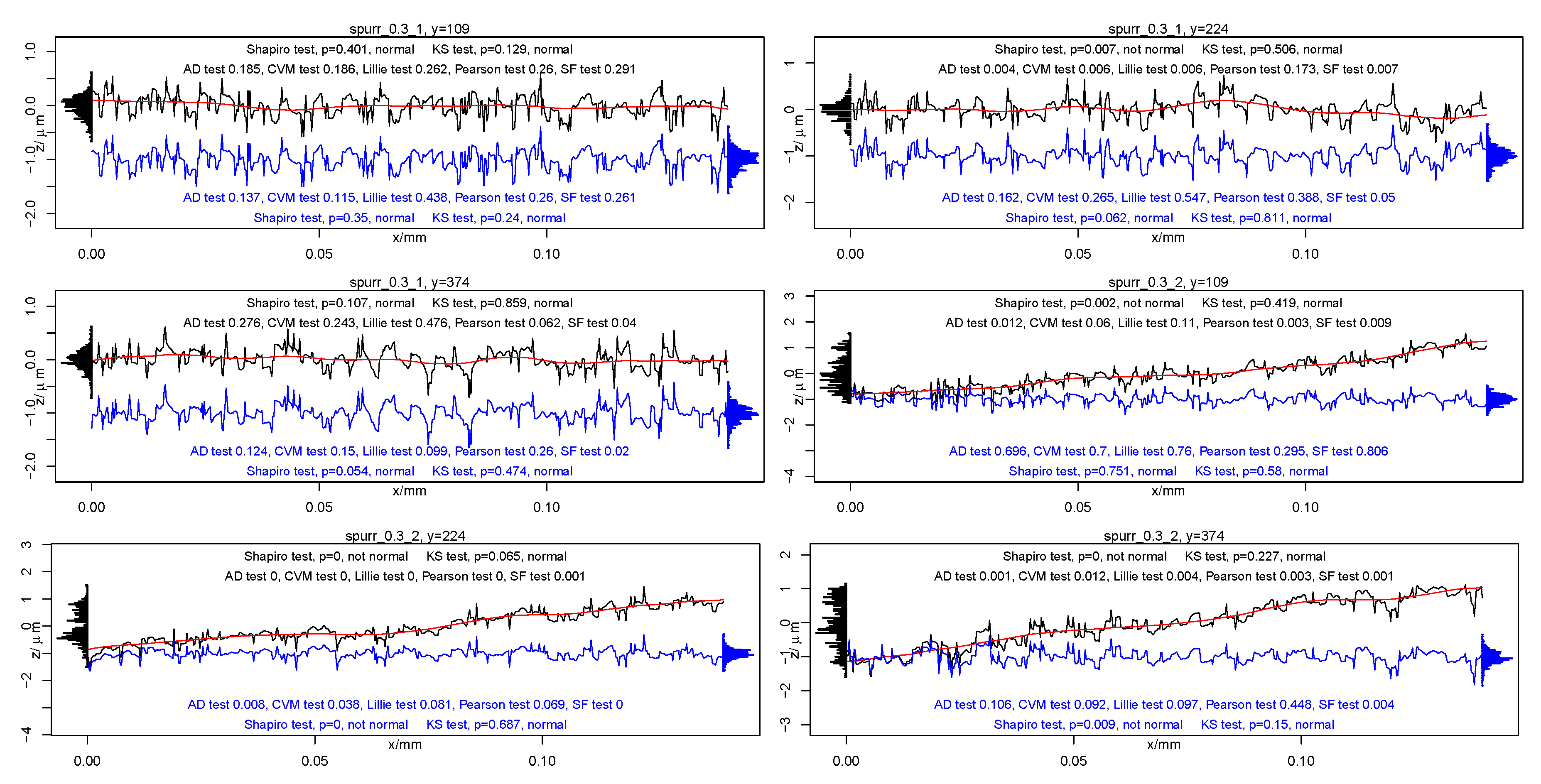
3.1. Normality Tests

As it has been shown above (see also a review in [21]), the crucial assumption of many models of contact is that the surface roughness is Gaussian. Hence, it is important to check if the height distribution of the tested surfaces follow the normal distribution. A large number of methods for testing for normality [46] has been developed. Each normality test is based on a particular test statistic that is used to give a quantitative estimation of proximity between an observed sample of measurements and the theoretical normal distribution. The assumption of normality is especially critical when characteristics of roughness profiles are derived. The main methods for testing for normality are the following tests: Kolmogorov–Smirnov (KS), Lilliefors (LF), Shapiro–Wilk (SW), Anderson–Darling (AD), Cramer–von Mises (CVM), the Pearson, and Shapiro–Francia (SF). Using the test statistic, each of the above tests produces a numerical characteristic that is called the p-value. This number characterizes the significance at the scale $[0,1]$ that the hypothesis of the normality is true for the observed measurements. One can nominate the acceptable significance level, say 5%. If the p-value is less than this level, then the hypothesis of normality should be rejected. Alternatively, if the number is within the significance level, then one can conclude that the height distribution is normal. Note that the acceptable significance level is a probability to reject the hypothesis of normality even if it is true.

To describe the tests, we introduce notations: $z_{\left(1\right)},\dots ,z_{\left(n\right)}$ is a permutation of the sample $z_1,\dots ,z_n$ such that $z_{\left(1\right)}\le \dots \le z_{\left(n\right)}$, $p_{\left(i\right)}=\Phi ((z_{\left(i\right)}-\overline{z})/s)$, where Φ is the cumulative distribution function of the standard normal distribution, and $\overline{z}$ and ${\mathsf{\sigma }}_s$ are mean and standard deviation of the sample.

3.1.1. The KS Test

The Kolmogorov–Smirnov (KS) test for a sample is based on comparison of an empirical distribution function (edf) $F_N\left(t\right)$ and the theoretical cumulative distribution function (cdf) $F\left(t\right)$ of the test distribution; specifically, the test statistic is

$$T=\underset{z}{max}|F\left(z\right)-F_{\mathrm{N}}\left(z\right)|,$$

where $F\left(z\right)$ is the cdf of Gaussian (normal) distribution and

$$F_N\left(z\right)=\left\{\begin{array}{cc}0,\hfill & z<z_{\left(1\right)},\hfill \\ i/n,\hfill & z_{\left(i\right)}\le z<z_{(i+1)},i=1,\dots ,n-1,\hfill \\ 1,\hfill & z\ge z_{\left(n\right)},\hfill \end{array}\right.$$

is the edf of the sample $(z_1,z_2,\dots ,z_N)$.

A limitation of the KS test is its high sensitivity to extreme values.

3.1.2. The LF Test

The Lilliefors (LF) test is a correction of the KS test in a way to be more conservative. The test statistic is the maximal absolute difference between the empirical and theoretical cdf as $D=max\{D^{+},D^{-}\}$, where

$$\begin{array}{c}\hfill D^{+}=\underset{i=1,\dots ,n}{max}(i/n-p_{\left(i\right)}),D^{-}=\underset{i=1,\dots ,n}{max}(p_{\left(i\right)}-(i-1)/n).\end{array}$$

The LF test is slightly better than the KS test because the LF test is more conservative.

3.1.3. The AD Test

The Anderson–Darling (AD) test is based on a squared difference between the edf and theoretical cdf, and the test statistic is

$$\begin{array}{c}\hfill Z=(1+0.75/n+2.25/n^2)\left(-n-\frac{1}{n}\sum _{i=1}^n(2i-1)(ln\left(p_{\left(i\right)}\right)+ln(1-p_{(n-i+1)}))\right).\end{array}$$

The Anderson–Darling test is sensitive to discrepancies in the tails of the distribution.

3.1.4. The CVM Test

The Cramer–von Mises (CVM) test is also based on a squared difference between the edf and theoretical cdf. The test statistic is

$$\begin{array}{c}\hfill W=(1+0.5/n)\left(\frac{1}{12n}+\sum _{i=1}^n{\left(p_{\left(i\right)}-\frac{2i-1}{2n}\right)}^2\right).\end{array}$$

The CVM test is uniform to discrepancies in different parts of the distribution.

3.1.5. The SW Test

The Shapiro–Wilk (SW, or Shapiro) test is based on the correlation between the data and the corresponding normal scores

$$\begin{array}{c}\hfill W=\frac{{\left({\sum }_{i=1}^n{c}_i{z}_{\left(i\right)}\right)}^2}{{\sum }_{i=1}^n{(z_{\left(i\right)}-\overline{z})}^2},c_i=\frac{m_i}{{\sum }_{j=1}^n{m}_j^2},\end{array}$$

where $m_i={\Phi }^{-1}((i-3/8)/(n+1/4))$. The Shapiro–Wilk test has better power than the KS test and the LF test. The Shapiro–Wilk test is known as the best choice for testing the normality of data.

3.1.6. The Pearson Test

The Pearson chi-square test is based on creating the classes built in such a way that they are equiprobable under the hypothesis of normality, where the number of classes is chosen as $m=2n^{2/5}$. The Pearson statistic is given by

$$P=\sum _{j=1}^m{(C_j-E_j)}^2/E_j,$$

where $C_j$ is the number of counted observations and $E_j$ is the number of expected observations under the hypothesis of normality in the j-th class.

3.1.7. The SF Test

The Shapiro–Francia (SF) test is simply the squared correlation between the ordered sample values and the (approximated) expected ordered quantiles from the standard normal distribution, and the test statistic is

$$\begin{array}{c}\hfill F=\frac{{\left({\sum }_{i=1}^n{\mathsf{\mu }}_i{z}_{\left(i\right)}\right)}^2}{{\sum }_{i=1}^n{(z_{\left(i\right)}-\overline{z})}^2},\end{array}$$

where ${\mathsf{\mu }}_i$ are standard normal ordered statistics.

3.2. Results of the Normality Testing

In Figure 3, we show the roughness analysis for data of the tested surface with nominal asperity size 0.3 $\mathsf{\mu }$m obtained by white light interferometer. The original profile measurements are given by a black curve. A waviness is shown by a red curve. The profile measurements with removed waviness are given by a blue curve. The height distribution for the original profile is depicted by a histogram on the left and for the profile with removed waviness on the right.

In Figure 4, we show the statistical analysis for roughness data of the tested surface with nominal asperity size 1 $\mathsf{\mu }$m. The meaning of notations is the same as in Figure 3.

Several tests for normality show that the height distribution is normal. One can observe that almost all p-values are greater that 0.05 and therefore we accept the hypothesis of normality for these measurements. Because, as it has been shown above, the surfaces with nominal asperity size 0.3 and 1 $\mathsf{\mu }$m do follow the Gaussian height distribution, it will be assumed further that the surfaces with higher nominal asperity sizes follow the same distribution.

Thus, we have confirmed normality of the height distribution of these intact surfaces of the replicas, i.e., the assumption of normality used by the above mentioned GW, FT and Galanov models of contact between rough surface was not violated for these surfaces. Hence, these models can be used for studies of the DSI tests of replicas of the intact surfaces of polishing paper.

4. The Indentation Tests of Epoxy Resin Replicas and Theoretical Modelling

4.1. Experimental Data Obtained by DSI

As it has been mentioned above, the force tester Basalt 01 was used in the DSI tests. Epoxy-resin replicas of a smooth glass surface and five rough surfaces were used as substrates. For measurements of adhesion forces, a micro-force tester equipped with a double-leaf spring serving as a cantilever beam was applied. Here, a soft spherical probe was pressed with a given force onto a sample. The required force to release the probe from the surface (pull-off force) corresponds to the adhesive property of the sample. If the surfaces were smooth, then, in the case of a spherical probe, the real contact area and effective elastic modulus could be calculated according to the Johnson–Kendall–Roberts (JKR) theory, which is a well established standard analyze method for micro-scale adhesion between elastic materials.

The JKR theory was developed for adhesive contact between two smooth elastic spheres or a rigid sphere and an elastic half-space (see for details [1,44,47]). However, here we consider contact interactions between relatively rigid epoxy resin replicas and a soft polydimethylsiloxane sphere. These are polymer materials. Properties of such materials are time-dependent and their elasticity is often described by Volterra integral equations [48]. However, if the kernel of the Volterra equation is not singular (the physical meaning of this condition is that the rearrangements of long polymer chains in both materials are not very fast), then, for short times for the loading–unloading tests, the materials may be quite often treated as elastic ones. Furthermore, adhesion of polymers may have different physical origin (see [49] and also a comprehensive review [50]). However, if the loading to the prescribed maximal compressive force and unloading of the samples take the same short amount of time for all samples, then it is quite convenient to use "the specific work of adhesion of contacting pair of materials" and use these values to compare the results of the tests.

The experimental absolute value of the pull-off force for replica of smooth glass surface was $P_{\mathrm{c}}^{\mathrm{exper}}=2845$ $\mathsf{\mu }$N. Absolute average values of measured pull-off forces are presented in the 4th column of

Table 2. The final outcomes of theoretical calculations in comparison with experimental results.

Nominal Size of Surface Asperities ($\mathsf{\mu }$m)	${\mathit{w}}_{\mathbf{rough}}$ [N/m]	${\mathit{P}}_{\mathbf{c}}^{\mathbf{rough}}$ [mN]	${\mathit{P}}_{\mathbf{c}}^{\mathbf{exper}}$ [mN]
$0.3$	$1.43$	$10.12$	$3.823$
1	$0.66$	$4.69$	$3.022$
3	$0.39$	$2.74$	$2.779$
9	$0.31$	$2.18$	$2.251$
12	$0.29$	$2.03$	$2.108$

. One can see that the highest average of the pull-off force value $P_{\mathrm{c}}^{\mathrm{exper}}=3823$ $\mathsf{\mu }$N was obtained not on the smooth sample, but on the rough surface whose nominal size of surface asperities was 0.3 $\mathsf{\mu }$m. The pull-off forces decreased continuously with the further increase of the surface micro-roughness [5].

4.1.1. Modelling of Surfaces as Random Process Graphs

Here, we will provide some theoretical justifications of the plausible explanation of the experimental data given in [5].

First, we note that the greater the area of the true contact, the stronger the adhesion absolutely irrespective to the nature and the value of the forces carrying out the adhesive connection [51]. Assuming that there is almost full contact between the smooth spherical probe and the tested surface for both the nominally flat sample and the surface having the nominal asperity size of 0.3 $\mathsf{\mu }$m, one can estimate the full area of the rough surface.

Of course the Galanov model has the same limitations as the Zhuravlev, GW, and FT models of discrete contact: it is assumed that contacts between asperities do not influence each other. Hence, if the rough surface of the nominal asperity size of 0.3 $\mathsf{\mu }$m has full contact with the probe, then the model cannot be applied. Let us estimate the total area of the rough surface.

Khusu et al. [13] studied several correlation functions for rough profiles having Gaussian height distributions. The asperity heights were calculated from the middle line of the profile, that, in turn, was calculated by the least square method. This was leading to introduction of additional parameters. Using this description, Linnik and Khusu [20] measured various parameters. In particular, they studied (i) the fraction of the horizontal line at a specific level, which lies within the roughness profile, i.e., they calculated the Abbott–Firestone curve, and (ii) the total area of the profile curve above this horizontal line. They reported pretty good agreement of the obtained results with their particular experimental observations. They suggested also to use the Abbe test for checking that the expectations of all values are the same, i.e., there are no trends in data. In addition to $K\left(x\right)$ of form in Equation (5), which is a correlation function of a homogeneous isotropic random field, they also studied the correlation function

$$K_2\left(x\right)=K_2\left(0\right)·e^{-{\mathsf{\alpha }}_2^2{x}^2},$$

(14)

where $K_2\left(0\right)$ and ${\alpha }_2$ are some parameters of the roughness. The correlation functions given by Formulas (5) and (14) will be used here to estimate the true area of rough surfaces.

From the real data of roughness over the rectangular (0.11 mm × 0.14 mm), we compute the number of summits N and the number of summits per unit area ${\mathsf{\eta }}_s$. Taking ${\mathsf{\sigma }}_s{\mathsf{\eta }}_{s}R=0.035$, one can calculate the radius of curvature of an asperity as $R=0.035/\left({\mathsf{\sigma }}_s{\mathsf{\eta }}_s\right)$. The results of calculations are presented in

Table 3. The parameters of the Galanov model.

Nominal Size of Surface Asperities ($\mathsf{\mu }$m)	N	${\mathsf{\eta }}_{\mathbf{s}}$ [${\mathbf{m}}^{-2}$]	R ($\mathsf{\mu }$m)	${\mathsf{\delta }}_{\mathit{c}}$ ($\mathbf{m}$)	${\mathit{P}}_{\mathbf{adh}}$ [N]	${\mathsf{\delta }}^{*}$
$0.3$	1975	$12.82·{10}^{10}$	$1.33$	$5.73·{10}^{-6}$	$2.52·{10}^{-6}$	$27.98$
1	1213	$7.87·{10}^{10}$	$0.79$	$4.83·{10}^{-6}$	$1.51·{10}^{-6}$	$8.62$
3	153	$0.997·{10}^{10}$	$2.06$	$6.64·{10}^{-6}$	$3.92·{10}^{-6}$	$3.90$
9	$10.8$	$0.07·{10}^{10}$	$12.08$	$12.2·{10}^{-6}$	$24.3·{10}^{-6}$	$3.13$
12	$8.2$	$0.053·{10}^{10}$	$15.0$	$12.9·{10}^{-6}$	$28.4·{10}^{-6}$	$2.92$

.

The calculations were fulfilled in the following steps.

Using the values of ${\mathsf{\delta }}^{*}$ obtained, we calculated the values of $w_{\mathrm{rough}}^{*}$ by Equations (11)–(13) of the Galanov model. Finally, we compute the specific adhesion work of rough surface $w_{\mathrm{rough}}=\mathsf{\sigma }{\mathsf{\eta }}_{\mathrm{s}}{P}_{\mathrm{c}}{w}_{\mathrm{rough}}^{*}$ and the real force of adhesion between a smooth sphere (probe) of radius $R_{\mathrm{s}}=1.5$ mm and rough surface as $P_{\mathrm{c}}^{\mathrm{rough}}=1.5\mathsf{\pi }{R}_{\mathrm{s}}{w}_{\mathrm{rough}}^{*}$.

The 4th column of Table 2 shows the average of the experimental pull-off force $P_{\mathrm{c}}^{\mathrm{exper}}$ [5]. These experimental values are close to the adhesion force given in the 3rd column calculated for contact between a smooth spherical probe of radius $R_{\mathrm{s}}=1.5$ mm and rough surface when the surface has nominal size of asperities larger or equal to 3 $\mathsf{\mu }$m. However, the calculated values $P_{\mathrm{c}}^{\mathrm{rough}}$ are not close to the experimental values for surfaces with nominal size 0.3 $\mathsf{\mu }$m and 1 $\mathsf{\mu }$m because there exists almost full contact and the Galanov model along with the FT or GW models are not applicable.

In the case of full contact, it is useful to compare the true area of the rough surface and the smooth one.

The length of a realization of a random Gaussian process $z\left(x\right)$ on a unite interval is

$$s=\frac{1}{L}{\int }_0^L{[1+z^{\prime 2}\left(x\right)]}^{1/2}\mathrm{d}x.$$

If the standard deviation of the process $\mathsf{\sigma }/L<<1$ and one employs the correlation function given by Equation (14), then one can write an asymptotic series for its expectation $Es$ (see Chapter 2.9 in [13]). It follows from Table 1 that rough profile having nominal asperity height 0.3 $\mathsf{\mu }$m has $\mathsf{\sigma }$ = 0.205 $\mathsf{\mu }$m over an interval $L=140$$\mathsf{\mu }$m, i.e., $\mathsf{\sigma }/L=0.205/140<<1$. Hence, the asymptotic series may be used. One can get that the estimations of the profile length are very small in the case if the correlation function given by Equation (14) is employed. We can conclude that Equation (14) does not reflect the horizontal distribution of asperities. However, our computations using numerical simulations of a Gaussian process with the exponential correlation function given by Equation (5) show that the length of the profile increases. Simulating the surface with the nominal size of asperities 0.3 $\mathsf{\mu }$m and computing the length of profiles along several lines, we have obtained that $s/L=1.16$. If we estimate the ratio of the true area of the rough surface to the nominal area as $A_{\mathrm{true}}/A_{\mathrm{nominal}}={(s/L)}^2$, then we obtain $A_{\mathrm{true}}/A_{\mathrm{nominal}}={1.16}^2=1.3456$. On the other hand, the ratio of $P_{\mathrm{c}}^{\mathrm{exper}}$ for the surface with nominal asperity heights 0.3 $\mathsf{\mu }$m to the pull-off force for the smooth one is $3.823/2.845=1.3438$. These ratios are in excellent agreement between each other. Thus, the plausible explanation of the observations given in [5] are correct and supported here by our theoretical considerations.

5. Conclusions

Currently, the design of many devices is influenced by discoveries of structures of biological objects. It is known that attachment organs of insects have worse performance at surfaces having specific roughness and this idea is used in preparation of the so-called anti-adhesive materials. To study effects of surface roughness on molecular adhesion between solids, it was suggested earlier to prepare epoxy resin replicas of surfaces having different roughness and conduct contact loading tests of the samples using a micro-force tester with a spherical smooth probe. Because the materials of all samples are the same, the roughness effects are not influenced by other factors. The contact loading tests between different samples showed a rather surprising results: a surface having very small roughness showed the greater values of the force of adhesion than the replica of a smooth surface. A plausible explanation of the observations was given in [5], suggesting that these rough surfaces had full adhesive contact while their true contact area is greater than the area for a smooth surface, and the surfaces with higher values of roughness do not have full contact.

One of the main purposes of the paper is to justify theoretically these explanations. Evidently, one needs to use a theory of adhesive contact between rough surfaces. Unfortunately, the main theories of contact between rough surfaces were developed for roughness whose height distributions are Gaussian. However, one cannot assume that the surfaces always have normal (Gaussian) roughness. For example, it was shown that the grinding surfaces are not Gaussian either at micro or nanoscale [21]. To check the assumption that the roughness is Gaussian, various modern tests of normality of data have been employed. These tests include the Kolmogorov–Smirnov, Lilliefors, Shapiro–Wilk, Pearson, Anderson–Darling, Cramer–von Mises and Shapiro–Francia ones. Of course, there are many other tests of normality (see a discussion in [46]). However, the tests used are the most popular ones. These tests showed that the height distribution of the surfaces under investigation are normal (Gaussian).

We can conclude that, for replicas of polishing papers, the exponential correlation function given by Formula (5) may be used to model horizontal distribution of asperities having Gaussian vertical distribution. The polydimethylsiloxane sphere is soft enough material to provide full contact for the surface with nominal asperity heights 0.3 $\mathsf{\mu }$m, while, for the used load, the full contact was not observed for surfaces having higher roughness. Using one of the Galanov models of adhesive contact between rough surfaces, the experimental observations are explained for surfaces whose nominal asperity values were over 1 $\mathsf{\mu }$m. For a surface with nominal asperity heights 0.3 $\mathsf{\mu }$m, we have provided the results of numerical simulations of random surfaces and justified the above explanations using geometrical arguments. Thus, the plausible explanation of observations have been theoretically justified.

References

1. Kendall, K. Molecular Adhesion and Its Applications; Kluwer Academic/Plenum Publishers: New York, NY, USA, 2001. [Google Scholar]
2. Eichler-Volf, A.; Kovalev, A.; Wedeking, T.; Gorb, E.V.; Xue, L.; You, C.; Piehler, J.; Gorb, S.N.; Steinhart, M. Bioinspired monolithic polymer microsphere arrays as generically anti-adhesive surfaces. Bioinspir. Biomim. 2016, 11, 025002. [Google Scholar] [CrossRef] [PubMed]
3. Fuller, K.N.G.; Tabor, D. The effect of surface roughness on the adhesion of elastic solids. Proc. R. Soc. Lond. A 1975, 345, 327–342. [Google Scholar] [CrossRef]
4. Gorb, E.; Haas, K.; Henrich, A.; Enders, S.; Barbakadze, N.; Gorb, S. Composite structure of the crystalline epicuticular wax layer of the slippery zone in the pitchers of the carnivorous plant Nepenthes alata and its effect on insect attachment. J. Exp. Biol. 2005, 208, 4651–4662. [Google Scholar] [CrossRef] [PubMed]
5. Purtov, J.; Gorb, E.V.; Steinhart, M.; Gorb, S.N. Measuring of the hardly measurable: adhesion properties of anti-adhesive surfaces. Appl. Phys. A 2013, 111, 183–189. [Google Scholar] [CrossRef]
6. Gorb, E.; Purtov, J.; Gorb, S. Adhesion force measurements on the two wax layers of the waxy zone in Nepenthes alata pitchers. Sci. Rep. 2014, 4, 5154. [Google Scholar] [CrossRef] [PubMed]
7. Borodich, F.M.; Galanov, B.A.; Gorb, S.N.; Prostov, M.I.; Prostov, Y.I.; Suarez-Alvarez, M.M. Evaluation of adhesive and elastic properties of materials by depth-sensing indentation of spheres. Appl. Phys. A Mater. Sci. Process. 2012, 108, 13–18. [Google Scholar] [CrossRef]
8. Borodich, F.M.; Galanov, B.A.; Gorb, S.N.; Prostov, M.Y.; Prostov, Y.I.; Suarez-Alvarez, M.M. Evaluation of adhesive and elastic properties of polymers by the BG Method. Macromol. React. Eng. 2013, 7, 555–563. [Google Scholar] [CrossRef]
9. Jiao, Y.; Gorb, S.; Scherge, M. Adhesion measured on the attachment pads of Tettigonia viridissima (Orthoptera, insecta). J. Exp. Biol. 2000, 203, 1887–1895. [Google Scholar] [PubMed]
10. Perepelkin, N.V.; Kovalev, A.E.; Gorb, S.N.; Borodich, F.M. Estimation of the elastic modulus and the work of adhesion of soft materials using the extended Borodich-Galanov (BG) method and depth sensing indentation. Mech. Mater. 2018, in press. [Google Scholar]
11. Galanov, B.A. Models of adhesive contact between rough elastic bodies. Int. J. Mech. Sci. 2011, 53, 968–977. [Google Scholar] [CrossRef]
12. Goryacheva, I.G. Contact Mechanics in Tribology; Kluwer: Dordreht, The Nederlands, 1997. [Google Scholar]
13. Khusu, A.P.; Vitenberg, Y.R.; Palmov, V.A. Roughness of Surfaces: Theoretical Probabilistic Approach; Nauka: Moscow, Russia, 1975. [Google Scholar]
14. Whitehouse, D.J.; Archard, J.F. The properties of random surfaces of significance in their contact. Proc. R. Soc. Lond. 1970, 316, 97–121. [Google Scholar] [CrossRef]
15. Maugis, D. Contact, Adhesion and Rupture of Elastic Solids; Springer: Berlin, Germany, 2000. [Google Scholar]
16. Nowicki, B. Multiparameter representation of surface roughness. Wear 1985, 102, 161–176. [Google Scholar] [CrossRef]
17. Whitehouse, D.J. The parameter rash—Is there a cure? Wear 1982, 83, 75–78. [Google Scholar] [CrossRef]
18. Abbott, E.J.; Firestone, F.A. Specifying surface quality: A method based on accurate measurement and comparison. Mech. Eng. 1933, 55, 569–572. [Google Scholar]
19. Meetings of the Town’s Mathematical Seminar in Leningrad. Uspekhi Mat. Nauk 1954, 9, 255–256. (In Russian)
20. Linnik, Y.V.; Khusu, A.P. Mathematical and statistical description of unevenness of surface profile at grinding. Bull. USSR Acad. Sci. Div. Tech. Sci. 1954, 20, 154–159. (In Russian) [Google Scholar]
21. Borodich, F.M.; Pepelyshev, A.; Savencu, O. Statistical approaches to description of rough engineering surfaces at nano and microscales. Tribol. Int. 2016, 103, 197–207. [Google Scholar] [CrossRef] [Green Version]
22. Zhuravlev, V.A. On question of theoretical justification of the Amontons-Coulomb law for friction of unlubricated surfaces. Proc. Inst. Mech. Eng. Part J J. Eng. Tribol. 2007, 221, 894–898. [Google Scholar] [CrossRef]
23. Kragelsky, I.V. Static friction between two rough surfaces. Bull. USSR Acad. Sci. Div. Tech. Sci. 1948, 10, 1621–1625. (In Russian) [Google Scholar]
24. Borodich, F.M. Translation of Historical Paper. Introduction to V A Zhuravlev’s historical paper: ‘On the question of theoretical justification of the Amontons-Coulomb law for friction of unlubricated surfaces’. Proc. Inst. Mech. Eng. Part J J. Eng. Tribol. 2007, 221, 893–898. [Google Scholar]
25. Greenwood, J.A.; Williamson, J.B.P. Contact of nominally flat surfaces. Proc. R. Soc. Lond. A 1966, 370, 300–319. [Google Scholar] [CrossRef]
26. Greenwood, J.A. Surface modelling in tribology. In Applied Surface Modelling; Creasy, C.F.M., Craggs, C., Eds.; Ellis Horwood: New York, NY, USA, 1990; pp. 61–75. [Google Scholar]
27. Polonsky, I.A.; Keer, L.M. Scale effects of elastic-plastic behavior of microscopic asperity contacts. J. Tribol. Trans. ASME 1996, 118, 335–340. [Google Scholar] [CrossRef]
28. Polonsky, I.A.; Keer, L.M. Simulation of microscopic elastic-plastic contacts by using discrete dislocations. Proc. R. Soc. A 1996, 452, 2173–2194. [Google Scholar] [CrossRef]
29. Borodich, F.M.; Savencu, O. Hierarchical models of engineering rough surfaces and bioinspired adhesives. In Bio-Inspired Structured Adhesives; Heepe, L., Gorb, S., Xue, L., Eds.; Springer: Berlin, Germany, 2017. [Google Scholar]
30. Johnson, K.L. Non-Hertzian contact of elastic spheres. The mechanics of the contact between deformable bodies. In Proceedings of the IUTAM Symposium; De Pater, A.D., Kalker, J.J., Eds.; Delft University Press: Delft, The Nederland, 1975; pp. 26–40. [Google Scholar]
31. Fuller, K. Effect of surface roughness on the adhesion of elastomers to hard surfaces. Mater. Sci. Forum 2011, 662, 39–51. [Google Scholar] [CrossRef]
32. Carpick, R.W. The contact sport of rough surfaces. Science 2018, 359, 38. [Google Scholar] [CrossRef] [PubMed]
33. Borodich, F.M. Fractal Contact Mechanics. In Encyclopedia of Tribology; Wang, Q.J., Chung, Y.-W., Eds.; Springer: Berlin, Germany, 2013; Volume 2, pp. 1249–1258. [Google Scholar]
34. Borodich, F.M.; Mosolov, A.B. Fractal roughness in contact problems. PMM J. Appl. Math. Mech. 1992, 56, 681–690. [Google Scholar] [CrossRef]
35. Borodich, F.M.; Onishchenko, D.A. Fractal roughness for problem of contact and friction (the simplest models). J. Frict. Wear 1993, 14, 452–459. [Google Scholar]
36. Borodich, F.M.; Onishchenko, D.A. Similarity and fractality in the modelling of roughness by a multilevel profile with hierarchical structure. Int. J. Solids Struct. 1999, 36, 2585–2612. [Google Scholar] [CrossRef]
37. Borodich, F.M. Similarity properties of discrete contact between a fractal punch and an elastic medium. Comptes Rendus L’Académie Sci. 1993, 316, 281–286. [Google Scholar]
38. Borodich, F.M.; Galanov, B.A. Self-similar problems of elastic contact for non-convex punches. J. Mech. Phys. Solids 2002, 50, 2441–2461. [Google Scholar] [CrossRef]
39. Borodich, F.M. Parametric homogeneity and non-classical self-similarity. I. Mathematical background. Acta Mech. 1998, 131, 27–45. [Google Scholar] [CrossRef]
40. Borodich, F.M. Parametric homogeneity and non-classical self-similarity. II. Some applications. Acta Mech. 1998, 131, 47–67. [Google Scholar] [CrossRef]
41. Galanov, B.A.; Valeeva, I.K. Sliding adhesive contact of elastic solids with stochastic roughness. Int. J. Eng. Sci. 2016, 101, 64–80. [Google Scholar] [CrossRef]
42. Galanov, B.A. Spatial contact problems for rough elastic bodies under elastoplastic deformations of the unevenness. PMM J. Appl. Math. Mech. 1984, 48, 750–757. [Google Scholar] [CrossRef]
43. Borodich, F.M.; Galanov, B.A.; Perepelkin, N.V.; Prikazchikov, D.A. Adhesive contact problems for a thin elastic layer: Asymptotic analysis and the JKR theory. Math. Mech. Solids 2018. [Google Scholar] [CrossRef]
44. Borodich, F.M. The Hertz-type and adhesive contact problems for depth-sensing indentation. Adv. Appl. Mech. 2014, 47, 225–366. [Google Scholar]
45. Borodich, F.M.; Galanov, B.A. Non-direct estimations of adhesive and elastic properties of materials by depth-sensing indentation. Proc. R. Soc. A 2008, 464, 2759–2776. [Google Scholar] [CrossRef] [Green Version]
46. Thode, H.C. Testing for Normality; Marcel Dekker: New York, NY, USA, 2002. [Google Scholar]
47. Johnson, K.L.; Kendall, K.; Roberts, A.D. Surface energy and the contact of elastic solids. Proc. R. Soc. Lond. A 1971, 324, 301–313. [Google Scholar] [CrossRef]
48. Rabotnov, Y.N. Elements of Hereditary Solid Mechanics; Mir Publishers: Moscow, Russia, 1980. [Google Scholar]
49. Kovalev, A.; Sturm, H. Polymer Adhesion. In Encyclopedia of Tribology; Wang, Q.J., Chung, Y.-W., Eds.; Springer: Berlin, Germany, 2013; pp. 2551–2556. [Google Scholar]
50. Myshkin, N.; Kovalev, A. Adhesion and surface forces in polymer tribology—A review. Friction 2018, 6, 143–155. [Google Scholar] [CrossRef] [Green Version]
51. Derjaguin, B.V.; Krotova, N.A.; Smilga, V.P. Adhesion of Solids; Consultants Bureau: New York, NY, USA, 1978. [Google Scholar]
Figure 1. The force-distance scheme for the classic unilateral contact and adhesive contact with a rough surface. The area of the grey-coloured zone is equal to the specific work of adhesion w rough .
Coatings 08 00350 g001
Figure 2. An example of the roughness image for surfaces with high nominal values of an asperity size (the nominal asperity size is 9 μ m). The white light interferometry was not able to provide data for considerable number of points.
Coatings 08 00350 g002
Figure 3. Roughness data of the tested surface with nominal asperity size 0.3 μ m obtained by white light interferometer: original data (black), waviness (red) and profile with removed waviness (blue); x-scale units are mm. The height distributions are given on the left and the right, respectively.
Coatings 08 00350 g003
Figure 4. Roughness data of the tested surface with nominal asperity size 1 μ m. The meaning of notations is the same as in Figure 3.
Coatings 08 00350 g004