
Detecting Anomalies in Financial Data Using Machine Learning Algorithms


Department of Computer Science, Electrical and Space Engineering, Luleå University of Technology, SE 971 87 Luleå, Sweden
*
Author to whom correspondence should be addressed.
Systems 2022, 10(5), 130; https://doi.org/10.3390/systems10050130
Submission received: 10 August 2022
/
Revised: 20 August 2022
/
Accepted: 22 August 2022
/
Published: 25 August 2022
Abstract
:Bookkeeping data free of fraud and errors are a cornerstone of legitimate business operations. The highly complex and laborious work of financial auditors calls for finding new solutions and algorithms to ensure the correctness of financial statements. Both supervised and unsupervised machine learning (ML) techniques nowadays are being successfully applied to detect fraud and anomalies in data. In accounting, it is a long-established problem to detect financial misstatements deemed anomalous in general ledger (GL) data. Currently, widely used techniques such as random sampling and manual assessment of bookkeeping rules become challenging and unreliable due to increasing data volumes and unknown fraudulent patterns. To address the sampling risk and financial audit inefficiency, we applied seven supervised ML techniques inclusive of deep learning and two unsupervised ML techniques such as isolation forest and autoencoders. We trained and evaluated our models on a real-life GL dataset and used data vectorization to resolve journal entry size variability. The evaluation results showed that the best trained supervised and unsupervised models have high potential in detecting predefined anomaly types as well as in efficiently sampling data to discern higher-risk journal entries. Based on our findings, we discussed possible practical implications of the resulting solutions in the accounting and auditing contexts.
1. Introduction
1.1. Research Relevance and Motivation
Nowadays, the application of machine learning (ML) techniques in financial auditing context is in high demand [1]. With ever-growing data amounts being processed in the enterprise resource planning (ERP) systems, the complexity of manual handling of audit-related tasks is extremely high and that requires better automation and smart solutions [2]. Business operations in companies and other business entities materialize in a traceable recording of financial transactions called bookkeeping, which is an essential part of financial accounting. Ease of manual work, error probabilities and material misstatement risk reduction while sampling and evaluating millions of financial transactions are sought to be addressed with applied machine learning [3].
Anomaly detection in accounting data is a routine of an auditor that reviews financial statements [4]. In general ledger (GL) data, business transactions are represented as journal entries. An atomic record that belongs to a unique journal entry is a transaction with an account type and corresponding attributes including among others a monetary amount and a debit-credit sign. A journal entry itself bears no information load about the transaction, while the combination of account types inside a journal entry creates financial activity patterns. Anomalies in these data include, but are not limited to, incorrect account type combinations, wrong corresponding monetary amount sign and abnormal amount proportions for the standard account patterns. Such deviations from standards in GL data may account for mistakes or intentional fraudulent activities [4].
Experienced auditors perform assessment of financial statements based on their professional knowledge by manually ’walking through’ sampled GL data, which is a labor-intensive task. Fundamental understanding of the data correctness in this case is limited to the scope of the well-known rules and regulations [5]. Moreover, random sampling of data means that the auditors’ focus area is dissolved and not every account will be examined. The auditors’ assessment work will result in identification of material misstatements and risky areas that overall describe a business entity financial performance [4]. In this case, a generalization problem emerges as there are limited known account patterns, errors and fraud scenarios while they also evolve with time.
A lack of advanced automated tools to equip auditors in their tasks triggers research in this area. Detecting anomaly data points by scanning through the whole transactions dataset and learning patterns, using supervised and unsupervised ML techniques, has a high potential to develop robust models helping auditors to concentrate on the risky areas drastically increasing their efficiency [2]. With more data science solutions being adopted by audit companies, expectations to lower audit costs while possibly increasing its quality also grow. Our motivation in this work is to contribute to this area of research by developing a GL data anomaly detection solution using and comparing a multitude of relevant ML techniques.
1.2. Problem Definition and Objectives
The constantly increasing volumes of accounting data, which need to be randomly sampled by auditors, picking just less than one percent of total for manual assessment, creates a sampling risk when financial misstatements dissolve in a much bigger non-sampled data group [3]. An auditor is limited in their ability to evaluate each misstatement case, especially when evolving fraudulent patterns are unknown, and that leads to failures in detecting intentional or unintentional financial misstatements [4]. To provide reasonable misstatements-free accounting data assurance is the auditor’s responsibility. Thus, intensified labor process has a direct cost impact on the auditing companies’ customers. Missing the detection of financial misstatements means missing mostly fraudulent statements, and as such, risks are higher, so the importance of the most accurate detection of data deviations cannot be underestimated [4]. To increase the efficiency of the accounting data auditing process and reduce related costs, the described problem needs to be addressed.
We were provided with anomaly-unlabeled general ledger data. Financial audit professionals have induced a small percentage of synthetic abnormal journal entries that are seen by the auditors as anomalies of the interest to be detected. The percentage of real data anomalies remains unknown, but presumably it is low, and we can deem original data to be anomaly-free. Each journal entry may contain a various amount of account transaction records which in isolation can abide by the standard accounting rules, while a certain combination of them can make a journal entry an anomaly. The aim of this work is to apply various supervised and unsupervised machine learning techniques to detect anomaly journal entries in the collected general ledger data for more efficient audit sampling and further examination.
To address the outlined problem, we defined the following research questions:
- Research question 1: Having GL data with journal entries of various sizes, how to use machine learning techniques to detect anomalies?
- Research question 2: How to enhance the configuration of machine learning models in detecting anomalies in the GL data?
2. Related Work
2.1. Anomaly Detection in Financial Data
In recent years, an increasing number of research papers were published that address anomaly detection in financial data using machine learning techniques. The vast majority of the ML applications focused on assurance and compliance, which includes auditing and forensic accounting [6]. Risk evaluations and complex abnormal pattern recognition in the accounting data remain to be important tasks where more synergistic studies contributing to this area are needed [2]. Compared to rule-based anomaly detection which is limited to manually programmed algorithms, the ML approach benefits from automatic learning and the detection of hidden patterns based on the labeled data or deviations from normality across the whole dataset that best suit the purpose of adaptation to data and conceptual drifts. Generally, extracted from ERP systems, both labeled and unlabeled real and synthetic general ledger data are used for these studies. Among the anomalies in financial data sought for detection are VAT-compliance violations, incorrect bookkeeping rules patterns, fraudulent financial statements, generic deviations from the norms and other errors [5]. Summing this up, the definition of anomaly in this context is irregular financial activity records, assuming that day-to-day financial operations are regular (normal) and result in regular records [4]. Examples of the taken approaches for anomalous accounting data detection were discussed in this chapter.
A supervised machine learning approach was taken for developing a framework to detect anomalies in the accounting data, as presented in [7]. A single company’s data were extracted from the ERP system to train and evaluate six different classifiers. The journal entry dataset comprised 11 categorical attributes, and the problem was set as a multi-class classification. The authors pointed out that many existing studies use traditional data analytics and statistics approach, and there is a lack of machine-learning applications. They concluded promising results and claimed high performance of the selected models based on multiple evaluation metrics and comparing the results with the established rule-based approach.
S. Becirovic, E. Zunic and D. Donko in [8] used cluster-based multivariate and histogram-based outlier detection on a real-world accounting dataset. The case study was performed on a single micro-credit company. The authors used a K-means algorithm on each transaction type separately to achieve better clustering results, so different numbers of clusters were formed for respective transaction types. A second approach was histogram-based. Anomaly data were introduced by adding synthetic outliers. A specific threshold of anomaly score was set. Some of the found anomalies that appeared to be out of financial audit interest were still considered by the algorithms as anomalous data. In the paper, it is outlined that clustering algorithm was a good candidate for such type of analysis, and authors discussed a real-time application of the histogram-based approach.
A number of big accounting companies have their own examples of developing proprietary ML-based anomaly detectors. Boosting auditors’ work productivity, EY developed an anomaly detection tool called the EY Helix General Ledger Anomaly Detector (EY Helix GLAD) [9]. A team of AI engineers and financial auditors worked on a solution to detect anomalies in the general ledger data. As per authors, the auditors manually labeled a vast amount of the journal entries to have reliable train and test datasets. ML models were trained using these data, and the models’ performance was validated by the auditors to ensure the quality of the anomaly detection tool. A successful ML model was a ‘black box’ in nature with an inability to explain prediction results, so the EY team developed an additional solution to explain the model.
One of the largest accounting services companies, PwC, developed a tool called GL.ai that is capable to detect anomalous data in the general ledger dataset using machine learning and statistical methods [10]. The solution scans through the whole dataset to assign labels to the journal entries considering a larger amount of attributes. Time dimension is considered when a transaction record is registered to identify time-wise unusual patterns. Outlying combinations of attributes and patterns are detected as anomalies and visualized. Anomaly detection is performed on different granularity levels, which allows for conducting an entity-specific analysis. Among the examined business entity financial activity features are account activity, approver, backdated registry, daytime, user and date.
M. Schreyer at al. in [11] trained an Adversarial Autoencoder neural network to detect anomalies in financial real-world data extracted from an ERP system. An assumption of ‘non-anomalous’ data was made for this dataset. Real-world and synthetic datasets were prepared and used in the training process, and records of synthetic anomalous journals were induced. Two types of the anomalies were established: global anomalies standing for having infrequently appearing feature values and local anomalies standing for an unusual combination of feature values. Autoencoder models learn a meaningful representation of data and reconstruct its compressed representation using encoder and decoder components. A combined scoring system was developed using adversarial loss and a network reconstruction error loss.
M. Schultz and M. Tropmann-Frick in [12] used a deep autoencoder neural network to detect anomalies in the real-world dataset extracted from the SAP ERP system for a single legal entity and one fiscal year. The analysis was performed on the per-account granularity selecting only Revenue Domestic, Revenue Foreign and Expenses. Anomaly journal entries were manually tagged by the auditors, and the labels were used in the evaluation process. Evaluation results were assessed in two ways. First, auto-labeled data were compared to the manual tagging performed by the auditors. Second, manual overview was done for those anomalies that were not manually tagged. The authors concluded that reconstruction errors can be indicative in finding anomalies in the real-world dataset.
A variational type of autoencoder in another study [13] was trained on the data extracted from the Synesis ERP system. Only categorical features were used in the training process. The authors evaluated model performance without labeled data based solely on the reconstruction error characteristics of the model.
2.2. Supervised and Unsupervised Machine Learning Techniques for Anomaly Detection
Machine learning, as a study of algorithms to learn regular patterns in data and their taxonomy, fundamentally includes supervised, unsupervised and semi-supervised types [14]. Supervised learning assumes labeled data instances to learn from, which declares a model’s desired output. Depending on the algorithm in use, a model is adjusted to predict classes or numerical values within a range. This corresponds to classification and regression problems, respectively. Supervised learning type is the most common [14]. The principal difference in unsupervised learning is the absence of labels that still can exist in the original data but that are not taken into account as a feature by this type of models. Output from unsupervised models is based on the test data-related properties understanding and findings, and the main goal is to extract data structure instead of specific classes. This includes distance and density-based clustering as a method to group data instances into ones with similar properties. Association rules mining also belongs to the latter type, while unsupervised neural networks can share place in a semi-supervised or self-supervised type of machine learning (as instances of different types of autoencoders). The selection of a machine learning model type for anomaly detection depends on the availability of labels and existing requirements for deriving unknown patterns [5].
Anomaly detection with supervised machine learning assumes labeled data. Each data instance has its own tag that is usually a human input about how the algorithm should treat it. Binary classification means dichotomous division of data instances into normal and anomalous, while multi-class classification involves division by multiple types of anomalous instances and normal data instances. Classification problematization takes a major part (67%) out of all other data mining tasks in the accounting context, and among the most used ML classifiers are logistic regression, support vector machines (SVM), decision tree-based classifiers, K-nearest neighbor (k-NN), naïve Bayes and neural networks [6].
In anomaly detection process with unsupervised machine learning, there is no target attribute (label) that is considered during a model fitting process. It is expected that scanning through the whole dataset, an automatic learning process will differentiate data instances that deviate from normality perceived by the model. In a setting where there are no labels or there may exist unknown anomaly patterns, it may be highly beneficial [3]. According to F. A. Amani and A. M. Fadlalla in [6], neural networks and tree-based algorithms are among the most used data mining techniques in accounting applications. In this work, we will focus on isolation forest (IForest) and neural network autoencoder as unsupervised anomaly detection methods.
3. Research Methodology
3.1. Algorithms Selection Rationale
The popularity of supervised and unsupervised machine learning techniques almost equally and linearly grows with time, while the performance of machine learning solutions depends both on the qualitative and quantitative data characteristics and a learning algorithm [15]. In this work, we implemented seven fundamental supervised ML techniques that can be adopted to build an ML classification model for outlier detection. We aimed to include such approaches as probabilistic statistical, high-dimensionality spaces adapted, non-parametric tree-based, non-generalizing, Bayes’ theorem-based and representation learning modeling. These techniques were successfully used in the financial accounting context [6]. We also implemented two cardinally different powerful unsupervised techniques, isolation forest and Autoencoder, that are broadly adopted in the industry.
All enlisted techniques can be used to detect anomalies in general ledger data. Supervised learning requires labeled data. In this work, we have a highly unbalanced dataset with a small percentage of introduced synthetic anomaly data-points. In addition to this complexity, the original dataset may contain some number of unlabeled anomalies. Unknown anomaly patterns are also of auditors’ interest to detect, while we seek to find those that are labeled. Unsupervised anomaly detection serves the purpose to detect rare data deviations from the norm that can potentially cover both labeled anomalies and unknown anomaly patterns. To keep a relevant balance of supervised and unsupervised modeling in this work, we refer to the study [6], where the prevalence of supervised learning in the accounting context is outlined.
3.2. Data Mining Frameworks
Data science projects in academia and industry share common data mining concepts having multiple processes and methods. To standardize these activities, a number of data mining methodologies were formalized. Commonly following similar steps, there are differences in steps granularity as well as how and when these methodologies are applied. According to the comprehensive survey in [16], we can distinguish the three most popular and broadly recognized methodologies, namely , and . In addition, methodology is getting attention, being highly customizable and providing support for projects that initially utilized other methodologies [17].
- SEMMA. SEMMA data mining methodology consists of five steps that defined its acronym. Sample, Explore, Modify, Model and Assess steps form a closed cycle that iterates from the start until the goal is achieved [18]. A reduced amount of steps and simplification makes this methodology easy to understand and adopt.
- KDD. KDD stands for Knowledge Discovery in Databases. While implementing 5 steps, there are Pre KDD and Post KDD steps recognized to understand the user’s goals and lastly to incorporate a developed solution into existing user processes. Through selection, preprocessing, transformation (data mining), data mining and interpretation (evaluation), a target analytical dataset is created followed by data cleaning, transformation and an analytical part evaluated in the interpretation step. In KDD, the steps are executed iteratively and interactively.
- CRISP-DM. Cross-Industry Standard Process for Data Mining (CRISP-DM) consists of 6 steps that start with business understanding and end with the deployment of a developed solution. Data-related tasks are handled in data understanding, data preparation and modeling assessed in the evaluation step. Iterations can be done throughout business understanding and until the evaluation step.
- TDSP. TDSP acronym stands for Team Data Science Process, which is Microsoft’s methodology to efficiently deliver predictive analytics and AI solutions [19]. It encompasses 5 steps, including 4 cyclic steps with bi-directional connections such as business understanding, data acquisition and understanding, modeling, deployments and the 5th customer acceptance step that signifies an end of a solution delivery cycle. In industry, along with agility of execution and teamwork in focus, it is highly beneficial to extend KDD and CRISP-DM with a customer acceptance criteria and a definite process for that.
According to the methodologies key aspects chart in [16], SEMMA methodology originated in an industrial setting and is based on KDD principles, while CRISP-DM is in a joint industry and academy setting and is based as well on KDD. CRISP-DM directly implements business understanding and deployment steps that are absent in both SEMMA and KDD. As well as being most popular and complete as stated in [18], CRISP-DM is flexible on reversing the direction of steps. While TDSP is well suited for industry, in academia we emphasize teamwork agility and customer acceptance less. In this work, we followed a standard CRISP-DM framework to efficiently and in a structured manner execute data mining activities.
In Figure 1, CRISP-DM steps are shown in sequence while iterations can be done as required and the order of how steps are executed can be reversed. This methodology is often depicted to center around data being an analytical subject. Reversing direction between steps is crucial when it is decided to adjust a previous step according to the current outcome. This flexibility well reflects real data science project processes as data and algorithm discoveries being made along the way that affects initial assumptions.
3.3. CRISP-DM Steps
- Business understanding. Understanding the business goal is a basis of any analytical process. Being unable to connect planned activities with the actual business objective leads to failures in evaluating the results and implementation of the developed solution. When a background is known, there is a need to define the objectives and success criteria. All this is not studied in a data-agnostic manner as it is crucial to understand that data required for the project can be extracted and processed.
- Data understanding. Data-centric processes require an understanding of how the data can be collected and what these data are, while mapping this knowledge with business understanding. During this stage, we describe collected dataset(s) and perform data exploration analysis. Data quality should be assessed and reported. Further data transformations should not be included in this step.
- Data preprocessing. Before data can be used in the modeling step, there are common transformations to be performed including data selection (sampling), data cleaning, feature selection, feature engineering and algorithm-required transformations such as reformatting, encoding, scaling, class balancing and dimensionality reduction.
- Modeling. The actual algorithmic part implementation is performed in this step. Having prepared input data, it becomes possible to train machine learning models or apply other statistical methods to achieve previously defined aim. In the case of machine learning modeling, algorithms and hyperparameters selection, composing and fitting the models are performed. The models’ performance assessment and obtaining the selected metrics values follow model training.
- Evaluation. Empirical results obtained in the previous steps need to be assessed, and if multiple models were trained, compared across the modeling step. Business success criteria identified in the business understanding step is taken into account. The overall success of the modeling process is discussed and a decision is being made on model selection and further steps.
- Deployment. If a solution ended up being successful, there may be a decision made to implement it in an existing setting. For machine learning modeling, a deployment plan is being developed including actual model deployment, maintenance and documentation. The deployment step may be used to distribute the gained knowledge about the data modeling in an organized manner [16]. In this case, it is limited to the discussion of contributing value of the developed solution in achieving the business goal, comparing the previous state of the problem in question in industry or academy and the implications of the applied solution.
4. Results
4.1. Business Understanding
In general ledger data, business transactions are represented as journal entries that contain transaction records along with other attributes including account number, monetary amount and debit-credit sign. Account number is a functional four-digit category that according to an account plan classifies a business transaction. In Sweden, the majority of the legal entities utilize a accounting plan that is structured according to the account position as account class, account group, control account, main account and sub-account [20]. The source attribute that is present in the data is a system that generated this bookkeeping data. Possible combinations of transactions inside a journal entry are expected to conform with standard rules (patterns), and deviations from the standards may account for unintentional or intentional fraudulent misstatements. To assure correctness of bookkeeping rules through the financial auditing process, auditors sample general ledger data and perform manual evaluations highly relying on their professional experience and data understanding. Financial misstatements are inevitably being missed due to the previously discussed sampling-risk and existing unfamiliar inconsistency patterns. Considering reviewed applications in industry and academia, there is big potential to solve this problem using statistical and machine learning methods.
General ledger data from several companies are being collected and were provided for this work. A small amount of synthetic anomaly journal entries were induced into the original dataset. There are multiple defined anomaly types, and each anomaly entry belongs to one of the types. These anomalies are of the auditors’ interest to detect. There are a number of factors that contribute to the auditor’s work complexity, including different sources which can be added or changed by companies, company and system-specific account plans, mixing industries with their own specifics of business transactions recording. Using the provided data, we will apply machine learning techniques to detect known and new anomalies to boost audit sampling efficiency.
4.2. Data Understanding
The provided general ledger data consist of journal entries collected from multiple companies with registered financial statements over different time periods. As seen in Table 1, the journal entry unique identifier is a categorical value that identifies a unique entry within a fiscal year for the specific company and registered on the effective date . A four-digit account number for a single transaction is contained in the field and accompanied by the monetary amount where the debit-credit sign is embedded. The field contains a source system categorical value.
Together with the described dataset attributes, we have labels. field contains a binary tag for a journal entry, where 0 stands for original data value and 1 accounts for a synthesized anomaly.
Along with binary-value label, we have a type of anomaly that is in the field. The field may contain values from 0 to 8 inclusively, so a non-anomalous entry will always have type 0, while the rest of the range corresponds to eight different anomaly types defined by the auditors. Table 2 shows data types for each column in the dataset. There are nine columns in total including two label columns and . Except labels, there are five categorical types, one datetime stamp and one continuous numeric type.
Each of the anomaly type entries is synthetically produced and joined with the original dataset. We assume normality of the original data and assign a 0 value for non-synthetic entries. However, according to the auditors’ opinion, original data may contain roughly up to 1–3 percent of anomalies. Anomalies that are contained in the original data can include those of the eight defined anomaly types as well as other deviations from the norm. Counts of induced anomaly types and original data entries are shown in Table 3.
There are 32,100 transactions in total, where 31,952 transactions are original data entries labeled as normal data. The rest of the entries are synthetically generated where for each type, we have from 14 to 22 transactions that account for anomalous journal entries. Total counts of normal and anomaly transactions as in Table 4 are 31,952 and 148, respectively, which is a percentage ratio 99.5389:0.4610. In this regard, we have a highly imbalanced dataset.
Synthetically induced data anomaly types have a definite description provided by the auditors presented in Table 5.
In the dataset, there are seven unique values for source systems and nine unique companies. In Table 6, the unique counts for all categorical data attributes are shown.
We can observe that there are 426 unique account numbers, which makes it a feature of high cardinality, while the rest of the high-cardinality attributes will be used to group transactions on journal entry level. As previously mentioned, a transaction on its own will not create booking patterns, but only transactions combination within a journal will. There are no records with missing values in the prepared data.
4.3. Data Preprocessing
4.3.1. Data Cleaning
We checked the dataset on existing missing values in the records, and there were none of such. Dropping duplicates was done to ensure we do not have any repeating records in the data. Data types of the columns were aligned, where categorical values became data types and effective date column became a type. We have only one continuous numerical column: . There are no values in the data that oddly do not correspond to the column they belong to.
4.3.2. Feature Selection
Feature selection is an important process that directly affects the modeling part success. According to the auditors, the core of understanding bookkeeping rules is account types in the column and a debit-credit sign that is to be created as a derived column from the value sign. Monetary amount can be useful in understanding ratios and monetary deviations, while for the data anomaly scope that is defined in Table 5, this feature has no relevance. In this work, we define an anomaly as a positive class with values of 1. Having attribute in the training model training process will potentially create monetary-based outliers that would increase the false-positive (false-anomalies) rate and will not contribute in finding anomalies of the described types. An effective date of the record in this sense will also create more distortion. The idea of using only categorical values for this purpose is supported in the published study [13].
4.3.3. Feature Engineering
Feature engineering is a broad term that includes existing feature transformation and generation of new features. In this subsection, we will explain simpler transformations, while more complex data manipulations are covered in the following subsections. As previously discussed, in our dataset we dropped a monetary amount column . A debit-credit sign is an important feature to find bookkeeping anomalies. We derived a sign from the column values and concatenated (debit) or (credit) with the values from a categorical feature . A new column that contains account number and debit-credit sign is called . Old column was dropped. Example values that are contained in the new column are , , etc. In Figure 2, we plotted a correlation matrix for the pre-engineered and post-engineered features, and labels using corresponding correlation/strength-of-association coefficients. After feature encoding, possible multicollinearity is resolved with the Principal Component Analysis technique.
4.3.4. Journal Entry Encoding
A journal entry consists of multiple transactions that belong to that entry. On its own, a journal entry is not informative. Only a combination of transaction records inside it create pattern to evaluate. The provided dataset is on the transactional level of granularity. A unique identifier of a journal is a compound key that must be created using , , . The source value from a column will become an attribute of a journal entry. It is important to make journal entries unique for training the model and reference back to the original data during evaluation. For each journal entry, we assigned a unique numeric identifier and we kept mapping keys for the new attribute.
The number of transactions inside a single journal entry can vary. In our dataset, the maximum number of transactions is four. Distribution of transaction numbers per journal is shown in Figure 3. As observed, more than 55% of all journal entries are bi-transactional, while three transactions per journal entry accounts for 36.3% of total. Only 7.3% of journal entries of the initial dataset contain as many as four transcactions.
To feed the training dataset into a machine learning model, we needed to vectorize journal entry data. The vectorization process is shown in Figure 4. We transpond each transaction record of a single journal entry so that all transaction features become attributes of the unique identifier of that entry. Padding is a method widely used in the data transformation process when data groups of differents sizes exist that need to be of an equal size for machine learning. Since we have journal entries of different sizes, we obtain vectors of padded sequences of a maximum journal entry size equal to 4 in our data. Each transaction itself contains its features that will add up to the vector.
4.3.5. Categorical Features One-Hot Encoding
Many machine learning techniques require categorical features to be encoded before they can be used to fit a model that require numeric values. Among these algorithms are decision tree-based, SVMs, linear models, neural networks, etc. One of the well-known and commonly used methods to number-encode categorical features is called one-hot encoding. Through this method, a discrete categorical feature is transformed to have a new column in a dataset for each unique value of the feature. The new columns are binary and can contain only true/false (1/0) values that accordingly correspond to presence of the category value for a particular data-instance. Original categorical columns after encoding are dropped. One-hot encoding produces sparse matrices/vectors that can drastically increase the dimensionality of an original dataset. In this work, we selected categorical features that need to be encoded. While a feature will not produce many columns after being one-hot encoded, high cardinality of an feature will largely increase the dimensionality of the original dataset. Among the other specifics of this process is that categorical feature encoding will lose value order information. In , there are multiple ways to perform one-hot encoding. One of the most simple is to call the pandas.get_dummies method that will transform all categorical features in the pandas dataframe; however, in this case we cannot separately encode unseen data for prediction using the trained model, which is usually an end goal of modeling. In this work, we use fit that can be stored and reused to encode new data.
4.3.6. Dimensionality Reduction
Real-world problems often require high dimensional data to be processed. Principal Component Analysis (PCA) is an unsupervised technique that decreases the number of columns in a sparse dataset using mathematical principles [21]. Through this technique, new features are created that are called principal components. These linearly uncorrelated components are derived as eigenvectors of the original data covariance matrix and explain their individual contribution to the total variance [21]. By picking a reduced number of new PCA-features, we reduce the original data sparsity.
As shown in Table 6, the feature had seven unique values and the feature contained 426 unique values. In subsection ‘Feature engineering’, we explained that we dropped the feature due to derivation of that increased the unique values in it to be 577 as some accounts may contain both debit and credit signs. After one-hot encoding of categorical features, we obtain a high dimensional feature-space of the size calculated as:
where N is the maximum number of transactions in journal entries, is a feature vector, is an feature vector and is a number of unique values in a feature F.
It is important to understand that data distribution of the features to be PCA-transformed and data normalization are recommended such as before applying PCA. Our data are binary, so centering the data is not required as the values can be only 0 or 1. In Figure 5, the left plot shows principal components’ cumulative explained variance for our sparse dataset after application of PCA.
The second plot (right) shows first 500 of the same principal components and a chosen cumulative variance threshold = 99% that is plotted as a vertical line. Generally, it is sufficient to take components that cumulatively explain up to 80% of variation [21], while in our case data explainability must be higher for the model to be able to learn and predict bookkeeping rules using one-hot encoded data. Using PCA, we were able to significantly decrease data dimensionaly still having features cumulatively of a very high variance explainability.
4.3.7. Data Normalization
Before we fit our ML model, we normalized the data so original feature values will be on the same scale. We used the method from the Python library to scale the data in a range from 0 to 1. The formula for feature scaling is as below:
where is a new range.
4.4. Modeling
We trained seven supervised and two unsupervised machine learning models using a different algorithm for each model to detect outliers in the preprocessed dataset. Supervised models will predict a dichotomous class that makes it a binary classification problem. In this section, we described empirical modeling processes and results.
4.4.1. Hyperparameters Tuning
Training machine learning models requires tuning algorithm-specific hyperparameters for the best performance of trained models. This usually is an iterative process that requires not only careful selection of parameters to be tuned, but also having a smarter automated method to efficiently iterate over complex hyperparameter spaces.
In this work, we used Python library to perform Bayesian optimization to tune hyperparameters over complex spaces of inputs [22]. Compared to simple grid search or random search, Hyperopt uses adaptive learning to concentrate on the best combinations of hyperparameters that makes the search process efficient. The algorithm minimizes a loss function and is highly customizable. Hyperopt requires defining an function running trials and an function where we pass a set of hyperparameters from the defined space and create an evaluation metric. Since Hyperopt minimizes the loss, to maximize an evaluation metric value, we assigned a negative value of this metric to the loss.
4.4.2. Train–Test Data Split
For supervised learning, we need to split the data into either train and test datasets, or train, test and validation datasets. The way the data should be split is highly dependent on data amount and other data properties among which are classes distribution. In our dataset, we have very few tagged anomaly classes compared to the total amount. Additionally, while we set a binary classification problem, we want our model to learn and be tested on each of the defined anomaly types. For an ML model, there exist unknown parameters that are to be identified from a train dataset while fitting the model [23]. The ratio of a train–test data split is important for the model performance. A. Gholamy, V. Kreinovich and O. Kosheleva in [23] pedagogically explained an empirically acknowledged balance of 70–30 or 80–20 percentage ratios. Having more labeled anomalies, it is reasonable to do a sensitivity analysis of a model performance for different train–test ratios. In our scenario, we split our data into two datasets that are train and test data with 70% and 30% of total, respectively. While splitting the data, we needed to stratify by the anomaly type, so equal proportions of each are present in the train and test data. For the purpose of reproducibility and proper models comparison, we have set a random state value while splitting.
4.4.3. Models Performance Measure
Binary classification models predict negative (0) and positive classes (1). In our work, we treat the anomaly class as positive. There are multiple classification metrics that can be calculated to evaluate binary classification models, and the most used are accuracy, precision, recall and F1-score [1]. These metrics can be calculated using a confusion matrix that is a result of values of a model’s predicted classes representation.
In Figure 6, a confusion matrix structure is explained in terms of true/false-positive and negative classes using actual class y-axis and predicted class x-axis position. Predicting a class by a trained ML model, we can extract values of corresponding , , and counts. All mentioned metrics can be calculated on the micro, macro average and weighted average levels. Choosing the right metrics for a model’s evaluation is problem- and class-balance-property-dependent. For instance, accuracy would not be a fair metric to evaluate a model on for a dataset with imbalanced classes, as in our case.
Below we compiled a comprehensive list of formulas to calculate metrics that we will discuss in this work:
In the list of Formula (3), recall, precision and F1 scores are calculated on a micro (class) level. Macro and weighted averages can be calculated using the last two formulas.
- Accuracy. The accuracy metric represents the percentage of correctly predicted classes, both positive and negative. It is used for balanced datasets when true-positives and negatives are important.
- Precision. Precision is a measure of correctly identified positive or negative classes from all the predicted positive or negative cases, when we care about having the least false-positives possible. Tuning a model by this metric can cause some true positives to be missed.
- Recall. Recall estimates how many instances of the class were predicted out of all instances of that class. Tuning a model using this metric means we aim to find all class instances regardless of possible false findings. According to [1], this metric is mostly used in anomaly and fraud detection problems.
- F1-Score. This metric mathematically is a harmonic mean of recall and precision that would balance out classes over or under representation to be used when false negatives and positives are important to minimize.
As we described for the recall metric, it is mostly used in finding anomalies. In the financial accounting setting, this addresses risks connected with missing financial misstatements. In this work, we used a recall average macro to tune and evaluate the models. In Figure 7, we showed four distinct cases of binary classes prediction resulting in a confusion matrices construction and corresponding evaluation metrics calculation. The support metric shows the real count of classes.
As seen from this figure, Case 2 is the most preferred in finding anomalous journal entries as we cover all the anomalies with the minimum false-positives. In Figure 7, we can observe that other metrics can be misleading given our problem. We used macro average of specificity and sensitivity to tune and evaluate our machine learning models. Further in this work, we refer to this metric as the recall avg macro.
4.4.4. Supervised Machine Learning Modeling
Logistic Regression Model
The basis of logistic regression is the natural logarithm of an odds ratio (logit) to calculate probabilities looking for the variables relationship [24]. Given the probabilistic nature of this algorithm, it is a relevant choice for prediction of classes (categorical variables) based on single or multiple, both categorical and continuous, features.
The probability of an outcome variable y being equal to 1 given a single x input variable is defined by the equation:
The model’s parameters a and b are the logistic function gradients. To handle more values, a general formula can be derived further as explained in [24].
To implement the logistic regression model, we have used class from Python library. This class uses different solvers that can be passed as a hyperparameter. The highest recall average macro value for the tuned logistic regression model is 0.943. The full classification report for the model shown in Table 8.
Two instances of an anomaly class were not discovered by the model. Missed anomaly types are shown in Table 9, where those that were misinterpreted were only anomalies of type 8. The model showed a high performance finding of 19 actual anomalies out of 21 and tagged 70 false-positive instances in the original dataset.
Support Vector Machines Model
Successful application of Support Vector Machines in a broad range of cases for classification problems made this algorithm among the ones to consider [25]. SVMs look up for optimal hyperplane(s) that would best separate data instances in the N-dimensional space using a maximized functional margin as a quality measure. Support vectors should be as far from the plane as possible to make the best classification predictor. The SMV decision function is defined as follows:
where for training samples (x), b is bias and y is a desired output. is a weighting factor and is kernel with a support vector .
In this work, we used classifier from Python library. It implements a one-vs.-all method for multidimensional space. The highest recall average macro value for the tuned SVM model was 0.965, which is higher than the Logistic Regression model results. The full classification report for the SVM model is shown in Table 10.
Only one instance of an anomaly class was not discovered by the model. The missed anomaly type is shown in Table 11, where the misinterpreted one was a type 8 anomaly, similar to the logistic regression model.
The best SVM model showed better coverage of true-positives, finding 20 actual anomalies out of 21, and additionally tagged 85 false-positives in the original dataset. A total of 85 misinterpreted class instances is a slight increase compared to logistic regression, while only manual quality check can attest to the usefulness of the presence of these false-positive predictions.
Decision Tree Model
Decision trees are classifiers that automatically create rules based on the learned data through scanning the dataset [26]. Classification tree output is categorical. Both categorical and numeric features can be used in the decision-based construction. The root node of the decision tree structure is a starting point from where subordinate decision (interior) nodes are constructed, where each non-leaf node division represents an attribute with split values. Feature testing and descending procedures are done throughout the whole tree construction until the leaf nodes. The most descriptive feature is prioritized in the splitting process based on entropy measure defined by the formula where is the proportion of the sample number of the subset and the i-th attribute value [26]:
The closer value to 0, the more impure the dataset is. On the opposite, information gain as an entropy reduction measure is used to determine a splitting quality aiming at the highest value. Its equation is as follows:
where attribute A range is , and a subset of set S is equal to the attribute v values [26]. Splitting the tree is terminated after no more value can be added to the prediction.
We implemented decision tree model using class from Python library. The highest recall average macro value for the tuned Decision Tree model is 0.985, which is higher than previously trained logistic regression and SVM models. The full classification report for the decision tree model is shown in Table 12.
The decision tree model discovered all the actual positive class instances while increasing negative class misclassification, obtaining more false-positives up to 107 instances. Achieving full prediction coverage of all actual anomaly instances serves the purpose of this work. We still need to keep track of increasing false-positive counts that we accounted for, looking into results of other well-performing models.
Random Forest Model
To address the overfitting problem of decision trees and improve performance, ensemble decision-tree based algorithms were introduced, and random forest is one of the most accurate and widely sused [27]. The idea behind random forest classifiers is to construct a multitude of decision trees and use a voting decision mechanism. Randomization comes from bagging and features random sub-setting. Bootstrapping allows trees to be constructed using different data, and with features subset selection, it results in two-way randomization; thus, weak learners are consolidated into a stronger ensemble model.
The highest recall average macro value for the tuned random forest model is 0.992, which outperforms previously trained models. A full classification report for the random forest model is shown in Table 13. There were no undiscovered true-positive class instances, and false-positive instances are fewer than in other trained models. The random forest model showed the best prediction power performance, while it was slower to train and tune compared to previously trained models.
K-Nearest Mean Model
K-nearest neighbor classifiers are based on assigning data instances to a class accounting for the nearest class data points [28]. One of the most used distance calculations is Euclidean:
where to calculate the distance between x and y datapoints in the n-dimensional space, a square root is taken from the sum of the squared differences for and . K-number in the algorithm is a number of considered nearest neighbors of the data points to be classified. For multiple classes instances, a voting mechanism decides on the classes majority. On the occasion of equality in the number of classes, they are picked at random or considering distance-based weights. Feature scaling is required for the algorithm treating in proportional feature contribution. K-values, a manually selected parameter and iteration over a range of k, is required to tune the k-NN classifier performance. Since calculation of all the distances is performed, all data instances should be kept in memory.
The single hyperparameter to tune in this model is the number of nearest neighbors. We used a range from 1 to 30 to iteratively test a model with different k-parameters. The highest recall average macro value for the tuned KNN model is lower compared to the previously trained models and is equal to 0.856. A full classification report for the KNN model is shown in Table 14. KNN models tend to overfit with low number of k, where we have the lowest possible value equal to 1. Compared to other discussed models, in KNN it is not possible to pass class weights, so classes imbalance negatively impacts model performance as it is sensitive to the over-represented class. In future work, the KNN model can be tested with balanced data.
There were 15 positive class instances correctly identified, while 6 were missed. Moreover, three false-positives were found. Missed anomaly types are shown in Table 15, where there are six instances of types 8, 6 and 1.
Artificial Neural Network Model
An artificial neural network (ANN) is a computational method utilizing interconnected artificial neurons as minimal computing units resembling human brain operation, and supervised learning is most commonly used to train ANN models [30]. The typical structure topology of neural networks is to have groups (layers) of multiple neurons with the first layer being an actual input of features received by the network and the last layer as a model’s output. Between input and output layers, there exists a hidden group of neurons. Deep architecture of ANNs involves more than one hidden layer. In a fully connected feedforward neural network, each neuron is connected to every neuron in the following layer. Weights of the neurons are typically being adjusted through backpropagation process when expected and produced outputs are compared. The iterative process of weights adjustment allows a neural network to learn on training data.
We have trained and compared the performance of three neural network models, starting with ‘vanilla’ ANN with one hidden layer and further increasing the number of hidden layers to build deep neural networks as shown in Figure 8. We used activation function for hidden layers and activation for output layers. We trained the models for 30 epochs with early stopping monitoring validation loss, with patience parameter equal to 3. This means that training stops when the monitored value does not increase during three epochs. loss and optimizer with the default learning rate equal to 0.001 were used when compiling the models. We passed class weights when fitting the models and used the validation dataset.
All three neural network models showed comparable prediction power. Their respective confusion matrices are plotted in Figure 9.
The best neural network model is selected by the highest recall average macro score (see Table 17). While all three neural network models performed very closely to each other, the third deep neural network showed a slight increase in true-positive counts. None of these models discovered all the anomaly classes. DNN2 missed 3 anomaly instances out of a total of 21 and tagged 6 false-positive instances.
4.4.5. Unsupervised Machine Learning Modeling
For unsupervised learning, we implemented two discussed models using an isolation forest algorithm and an autoencoder neural network. To decrease noise in the data and for better unsupervised separation of data instances, we used the first two digits of the feature . We apply principal component analysis method in the data transformation pipeline, while the models showed better performance efficiency when PCA components were kept to the maximum, where we have maximum variance explainability.
Isolation Forest Model
Notably, the isolation forest (IForest) algorithm was specifically created for an anomaly detection task, and it differs from other approaches by explicit isolation instead of profiling the usual data points [31]. Binary trees are constructed by the algorithm, and anomaly scores are distance-based, meaning that isolation of anomalies should be easier than the usual data-instances that have shorter distances [32]. Recursive process selects random feature and a random feature values to split on that is within the feature range. The anomaly score deterministic factor is the tree-path distance to achieve the split of the scored data-point. Among other advantages of IForest is computational time as the complexity is approximately linear and the ability to handle high-dimensional data [31].
The anomaly score equation is given as:
where S is anomaly score for point x and the average of is , which is an average of all tree depths of a data-point. In the denominator, is a mean tree depth of an unsuccessful search calculated as follows:
where n is a total number of data points and is a harmonic number calculated by a summation of and . An average score for each data-point across all trees is the final anomaly score estimate.
To implement the isolation forest model, we used class from Python library. For this model, the whole dataset is scanned to find anomalies across it in an unsupervised mode.
estimates anomaly scores according to the parameter value that we set to ‘auto’. We do not consider this threshold in our analysis. Instead, we use Tukey’s method to test the univariate range of anomaly scores for outliers.
In Figure 10, we plotted the model’s anomaly scores per actual anomaly binary class Figure 10a and per types of anomalies Figure 10b. For both plots, 0 is a negative non-anomalous class. The dotted horizontal line is a statistically calculated threshold using Tukey’s method.
We can observe a distinct separation of the actual anomalous instances by the threshold line, while there is a part of the actual non-anomalous data instances outliers that is below the line. For evaluation purposes, we found the maximum anomaly score among actual anomalies to set as a threshold value separating anomalous and normal data points.
Autoencoder Model
Autoencoders are the most used NN-based anomaly detection methods, and neural networks are prevailing to detect anomalies in accounting data according to [3]. G. Pang et al. in [33] pointed out that Autoencoder-based anomaly detection can address four out of six main anomaly detection challenges, namely: low anomaly detection recall rate, high features-dimensionality, noisy data and highly complex features relationships. Among weaker points for autoencoders is data-amount depending efficiency and explainability.
Autoencoder is an unsupervised method where an artificial neural network automatically learns compressed semantic representation of the data and is able to reconstruct it back so the input and output are the same [34]. Autoencoders are a bi-component, and the first component is called encoder. In the encoder part, the neural network learns on the whole data through multiple layers of declining size till the compressed data representation is achieved. The second part called decoder reconstructs the original input from the compressed representation through inclining layers usually mirrored from the encoder. The encoder does not just remember the original data as its last compressed layer is a model’s bottleneck with non-linearly learned semantics. There is no train–test data split that is required for this type of learning, and the whole dataset is passed while fitting the model. Autoencoder architecture requires the same whole dataset to be used twice, once as train data being an input and once as test data acting as the ground truth.
To implement the autoencoder model, we used API from machine learning platform. Autoencoder must contain encoder and decoder parts. Deep neural network composition was used for each of them. We created a class to assemble encoder-decoder parts and a function to return decoded output. We trained the model for 50 ephocs with the default learning rate = 0.001 and provided validation data to the fit function, while batch size was set to 1. The two-part model composition is shown in Figure 11.
For the encoder’s model part, we created four hidden layers with 128, 64 and 16 neurons for dense layers and 8 neurons for the last dense latent space layer, respectively. Activation function is used to introduce non-linearity. The decoder part consists of four dense layers with 16, 64, 128 and 512 neurons and the same activation function except using for the last output layer. The training process is plotted in Figure 12, where we observe training and validation losses decreasing synchronously with epochs.
Lower levels of anomaly scores would signalize about anomalous data instances. Similar to isolation forest, for the autoecnoder model in Figure 13, we plotted the model’s anomaly scores per actual anomaly binary class in Figure 13a and per types of anomalies in Figure 13b. For both plots, 0 is a negative non-anomalous class. The dotted horizontal line is a statistically calculated threshold using Tukey’s method.
The majority of data points are below the threshold line, while very few are above. Some false-positives are also below the line, meaning that they are tagged as anomalies. For evaluation purposes, we found the maximum anomaly score among actual anomalies to set as a threshold value separating anomalous and normal data points. Compared to the isolation forest model, the autoencoder model performed lower with recall average macro equal to 0.9441. False-positive counts are higher and are equal to 1421 instances, while for isolation forest they were equal to 1130.
4.5. Evaluation
We measured and compared the models’ performances based on the selected performance metric together with the confusion matrices overview. Besides how statistically accurate the trained models are, there are other criteria that can be considered such as interpretability, operational efficiency, economical cost and regulatory compliance, as outlined in [1].
4.5.1. Supervised Models Evaluation
For supervised modeling, we trained logistic regression, support vector machines, decision tree, random forest, K-nearest mean, naïve Bayes and Artificial Neural Network models. All the models except the K-nearest mean model were optimized using a Hyperopt Bayesian optimizer with 100 iterations searching for the best model hyperparameters in the defined search space. That means that 100 different models were trained using each machine learning algorithm implemented with Hyperopt optimization, performing an efficient search for the best values. The K-nearest mean model is implemented with a simpler iteration over the range of K-values from 1 to 30. To ensure an unbiased train and evaluation process, we used a stratified split by anomaly type. In this scenario, an equal percentage of each anomaly type instance ended up in each of the splits. In the Hyperopt optimization trials object, we stored the model hyperparameters and corresponding classification report metrics. Finally, from each of the seven model optimization trials of multiple iterations, we selected the seven best-performing models based on the selected performance metric. In Table 18, we compared seven tuned models listing their true-negatives (TN), false-negatives (FN), false-positives (FP) and true-positives (TP) counts and recall average macro metric values.
Based on the selected evaluation criteria, the random forest ensemble algorithm showed the best performance. While not missing any of the actual anomaly journal entries (true-positives), it also tagged as anomaly a minimum number of the non-anomalous data instances (false-positives) compared to the rest of the trained models. Performance-outsider is a naïve Bayes model that discovered only 4 out of 21 anomaly instances. The K-nearest neighbor algorithm showed the second worst results with the best k-value equal to 1, which is a sign of probable overfitting. The second best model that covered all the anomalous journal entries is the decision tree; however, it misinterpreted the highest amount of the actual true-negatives. Overall, with the best trained supervised machine learning model (random forest), we were able to achieve a full predictive coverage of the anomalous data instances while misinterpreting a reasonable amount of non-anomalous data points (1.48% out of total).
4.5.2. Unsupervised Models Evaluation
The isolation forest and autoencoder neural network that we trained to find anomalies in the general ledger data are unsupervised learning techniques. The main difference with supervised learning is that the patterns learning process does not require labeled data. However, for evaluation purposes, we used the class labels to calculate evaluation metrics based on the constructed classification report. Isolation forest and autoencoder models produce an anomaly score for each instance of the dataset. On this basis, we found the anomaly score thresholds statistically using Tukey’s method. The thresholds were then used to split data into anomalous and non-anomalous data instances. These thresholds are model-dependent and without knowing the ground truth, labels should be used to tag the instances in an unsupervised manner. In Figure 10 and Figure 13, we plotted data class separation and anomaly types separation across anomaly score y-axes using statistically defined thresholds for the respective models.
For the model performance comparison purpose using labels, we took the maximum anomaly score value in the vector of actual anomalous instances (true-positives) and made that a data separation point. Doing this for each of the two models, it is possible to make a fair comparison on how well the models perform. We constructed confusion matrices with true-negatives (TN), false-negatives (FN), false-positives (FP) and true-positives (TP) counts and calculated the recall average macro metric values shown in Table 19.
To give an estimate of how large the minimal sample of original data a model takes to cover all of the actual anomalous data instances (true-positives), we added the Anom.% column where this amount is calculated. As can be seen in Table 19, the isolation forest model showed a higher performance. It was able to discover all the actual anomalies including all anomaly types taking the minimum sample of data that amounts to 9.38% out of total. A close but lower performance showed the autoencoder model.
4.6. Deployment
In the deployment step, we discuss practical implications of our findings and possible transformations of audit analytics as of today using developed machine learning solutions. Consulted by the audit professionals, we analyzed the current state of audit processes that correlates with the problematization in this work. Below we enlist in no particular order existing challenges and discuss how individual auditors or audit companies can benefit from the deployed data science solutions that resulted in this work, addressing these challenges.
- Sampling risk. Manual assessment of financial statements requires random data sampling that practically amounts to less than 1 percent of the total, with high probability that undiscovered misstatements will come into a bigger non-sampled group [3]. In this work, we trained an unsupervised machine learning model using the isolation forest algorithm that is capable to discover all anomalies of each of the defined anomaly types, sampling less than 10% of the most deviated data out of total. The anomaly score threshold can be adjusted, while in this work we set it using a statistical method. A ‘sampling assistant’ application can be created based on this model.
- Patterns complexity. According to the auditors, there exists a high complexity of patterns in the financial data. Different systems that generate these data and different individual account plans contribute to that problem. Besides, multiple transaction types are grouped into a single journal entry of different sizes. Leveraging size variability with data encoding, we trained a random forest machine learning classifier model that efficiently learns data patterns using labeled anomalies. The model is able to discover all anomalies of known types from the unseen test data, while tagging just 1.48% false-positives out of total data amount. Productionization of a high-performing supervised machine learning model allows automatic discovering of data instances of known anomaly types in the multivariate data.
- Data amount and time efficiency. Increasingly large data amounts make laborious manual auditing work more costly. Adopting machine learning solutions that help the auditing process can much decrease data-processing time and accordingly reduce associated costs. A deployed supervised anomaly detection model that we trained, depending on the system compute power, can make large batch predictions for the transformed data instantaneously that could help auditors to detect misstatements in record time. An unsupervised anomaly detection model would take comparably longer time scanning through the whole dataset, still providing results in a highly efficient manner compared to conventional methods.
- Imperceptibly concealed fraud. Each year, a typical legal entity loses 5% of its revenue because of fraud [1]. Evolving fraudulent financial misstatements are carefully organized, aiming to dissolve in the usual day-to-day financial activities. Conventional auditing methods inevitably create high risks of missing financial misstatements when the majority of missed misstatements are fraudulent [4]. The isolation forest unsupervised model that we implemented in this work is capable of discovering unknown patterns that deviate from normality of the data. Looking into high-risk data samples could more efficiently reveal concealed fraud.
- Deviation report. Accounting data deviation report can be based on multiple data science solutions. Provided that we trained an unsupervised anomaly detection model that scans through all journal entries, it is possible to show which data instances are deviating from normality based on the selected anomaly score threshold. Moreover, each data point is assigned with the anomaly score, so there exist a possibility to group journal entries by risk levels.
5. Discussion
Along with the initially unlabeled general ledger data, the audit professionals provided us with the small amount of synthesized anomalous journal entries of the specific types, while we assumed normality of the original data. We applied supervised and unsupervised machine learning techniques to learn on labeled data and detect anomalous data instances. Following the steps of CRISP-DM, we trained and evaluated machine learning models.
In total, we trained seven supervised and two unsupervised machine learning models using different algorithms. In unsupervised modeling, a model training process is label-agnostic. When we trained unsupervised models, we used labeled data to calculate metrics. This allowed us to use the same evaluation criteria that we selected for the supervised model performance evaluation.
Among the seven compared supervised learning models, a random forest model performed the best, discovering all the anomalous instances while keeping at minimum false-positives. Among the two compared unsupervised anomaly detection models, the isolation forest model showed the best results. Notably, both of the best selected supervised and unsupervised models are tree-based algorithms.
Both random forest and isolation forest algorithms are highly efficient in a multidimensional space [27,31], and the trained supervised model can be used for real-time predictions, while the unsupervised isolation forest model requires more time to fit using the whole dataset. Both of the models were implemented and can be operated in Python programming language using open-source libraries.
Research Questions Re-Visited
Given the nature of the general ledger data, we got certain earlier discussed data-related challenges including variability of journal entry sizes and a relatively small percentage of the induced anomalies. The data preparation process included multiple steps. We first selected and engineered categorical features. To tackle the machine learning models’ requirement for the feature vector being of the same size, we performed journal entry data encoding. One-hot-encoding of high-cardinality features produced a sparse dataset that was leveraged with PCA-based dimensionality reduction.
To detect known types of anomalies, we trained supervised machine learning models using stratified data splits. We tuned hyperparameters of the trained models and during the evaluation step selected the best model using defined performance evaluation criteria. The random forest classifier model showed the best performance and was capable to discover 100% of all labeled anomalies in the unseen data while finding a minimal number of false-positives. As an alternative machine learning method to efficiently find unknown anomalous data instances across the whole dataset, we used an unsupervised learning approach. The isolation forest unsupervised anomaly detection model was able to discover all anomaly types while sampling only 9.38% deviating data of the total.
Overall, we conclude that using selected supervised and unsupervised ML models has a high potential to efficiently auto-detect known anomaly types in the general ledger data as well as sample data that most deviated from the norm.
Machine learning models with default parameters were used as an intuitive base-line reference. In this work, we implemented Hyperopt Bayesian optimizer that efficiently searches for the best models’ parameters across the defined search space. While tuning hyperparameters, it is required to iteratively evaluate the model’s performance. We selected a relevant performance measure that was used to consistently compare the trained models. In the financial accounting setting, controlling the recall average macro metric would leverage risks connected with missing financial misstatements. During models optimization, we aimed to increase the metric value to detect the most possible amount of actual anomalies (true-positives) and control for keeping false-positive discoveries at a minimum level.
The highly imbalanced dataset that we dealt with makes the models account the most for the over-represented class during a learning process, leading to decreased model performance. To address this, we used calculated weights of the classes distribution to fit the models.
Having implemented the model enhancements during the modeling part enabled us to better address the aim of this work.
6. Conclusions and Future Work
In this work, we have shown how to use supervised and unsupervised machine learning techniques to find anomalies in general ledger data. We also demonstrated how to enhance the models in order to improve their performance. The random forest and isolation forest models showed the highest performance. We limited the selected features to categorical only, since the defined anomaly types required to search for the combination patterns related only to categorical features. In future work, there can be other features or their combinations tested, including a monetary amount feature and a timestamp feature, depending on the anomaly types of interest.
The imbalance of classes was addressed by calculating and passing class weights to the models. There are other techniques that can address it, including SMOTE and ADASYN synthetic oversampling methods. They can be tested in future work to compare models’ performances. As well, a bigger number of labeled data anomalies would contribute to quality of future experimentation.
Additionally, data preprocessing is a key step where we have implemented data encoding to transform groups of transactions into 1-D arrays. The groups can be of various sizes, so we implemented a padding method. Our dataset contained journal entries with a maximum size of four transactions. Even though that size would cover a majority of the entries, in GL data there can be lengthier journal entries. To address this, either a different encoding approach should be used or additional data preparation needs to be implemented for the lengthier journals such as sliding window encoding. Furthermore, transactions that belong to journal entries can be seen as timesteps of the multivariate data of various sizes. Recurrent neural networks such as LSTM or GRU can be tested using this approach in future work.
For better loss estimate generalization, it can be practical to use a data re-sampling technique. One example of that is a K-fold cross-validation (CV) method, with k-times random data split where a hold-out (test) data amounts for . In our setup, as it is also discussed in [22], we considered avoiding CV while tuning the models to evade excessive processing times when the value of looking up the right hyperparameters may prevail. We have left experimentation with the concurrent implementation of re-sampling techniques and Hyperopt optimization for further studies.
Finally, under time constraints, we implemented only two unsupervised models where more algorithms and different model compositions can be applied.
Author Contributions
Conceptualization, A.B. and A.E.; methodology, A.B. and A.E.; software, A.B.; validation, A.B. and A.E.; investigation, A.B.; data curation, A.B.; writing—original draft preparation, A.B.; writing—review and editing, A.B. and A.E.; visualization, A.B.; supervision, A.E. All authors have read and agreed to the published version of the manuscript.
Funding
This research received no external funding.
Institutional Review Board Statement
Not applicable.
Informed Consent Statement
Not applicable.
Data Availability Statement
Not applicable.
Conflicts of Interest
The authors declare no conflict of interest.
References
- Baesens, B.; Van Vlasselaer, V.; Verbeke, W. Fraud Analytics Using Descriptive, Predictive, and Social Network Techniques: A Guide to Data Science for Fraud Detection; Wiley: New York, NY, USA, 2015. [Google Scholar]
- Zemankova, A. Artificial Intelligence in Audit and Accounting: Development, Current Trends, Opportunities and Threats-Literature Review. In Proceedings of the 2019 International Conference on Control, Artificial Intelligence, Robotics & Optimization (ICCAIRO), Athens, Greece, 8–10 December 2019; pp. 148–154. [Google Scholar]
- Nonnenmacher, J.; Gómez, J.M. Unsupervised anomaly detection for internal auditing: Literature review and research agenda. Int. J. Digit. Account. Res. 2021, 21, 1–22. [Google Scholar] [CrossRef]
- IFAC. International Standards on Auditing 240, The Auditor’s Responsibilities Relating to Fraud in an Audit of Financial Statements. 2009. Available online: https://www.ifac.org/system/files/downloads/a012-2010-iaasb-handbook-isa-240.pdf (accessed on 18 April 2022).
- Singleton, T.W.; Singleton, A.J. Fraud Auditing and Forensic Accounting, 4th ed.; Wiley: New York, NY, USA, 2010. [Google Scholar]
- Amani, F.A.; Fadlalla, A.M. Data mining applications in accounting: A review of the literature and organizing framework. Int. J. Account. Inf. Syst. 2017, 24, 32–58. [Google Scholar] [CrossRef]
- Lahann, J.; Scheid, M.; Fettke, P. Utilizing Machine Learning Techniques to Reveal VAT Compliance Violations in Accounting Data. In Proceedings of the 2019 IEEE 21st Conference on Business Informatics (CBI), Moscow, Russia, 15–17 July 2019; pp. 1–10. [Google Scholar]
- Becirovic, S.; Zunic, E.; Donko, D. A Case Study of Cluster-based and Histogram-based Multivariate Anomaly Detection Approach in General Ledgers. In Proceedings of the 2020 19th International Symposium INFOTEH-JAHORINA (INFOTEH), East Sarajevo, Bosnia and Herzegovina, 18–20 March 2020. [Google Scholar]
- EY. How an AI Application Can Help Auditors Detect Fraud. Available online: https://www.ey.com/en_gl/better-begins-with-you/how-an-ai-application-can-help-auditors-detect-fraud (accessed on 22 April 2022).
- PwC. GL.ai, PwC’s Anomaly Detection for the General Ledger. Available online: https://www.pwc.com/m1/en/events/socpa-2020/documents/gl-ai-brochure.pdf (accessed on 22 April 2022).
- Schreyer, M.; Sattarov, T.; Schulze, C.; Reimer, B.; Borth, D. Detection of Accounting Anomalies in the Latent Space using Adversarial Autoencoder Neural Networks. In Proceedings of the 2nd KDD Workshop on Anomaly Detection in Finance, Anchorage, AK, USA, 5 August 2019. [Google Scholar]
- Schultz, M.; Tropmann-Frick, M. Autoencoder Neural Networks versus External Auditors: Detecting Unusual Journal Entries in Financial Statement Audits. In Proceedings of the 53rd Hawaii International Conference on System Sciences, Maui, HI, USA, 7–10 January 2020. [Google Scholar]
- Župan, M.; Letinić, S.; Budimir, V. Journal entries with deep learning model. Int. J. Adv. Comput. Eng. Netw. IJACEN 2018, 6, 55–58. [Google Scholar]
- Ayodele, T. Types of machine learning algorithms. New advances in machine learning. New Adv. Mach. Learn. 2010, 3, 19–48. [Google Scholar]
- Sarker, I.H. Machine Learning: Algorithms, Real-World Applications and Research Directions. SN Comput. Sci. 2021, 2, 160. [Google Scholar] [CrossRef] [PubMed]
- Plotnikova, V.; Dumas, M.; Milani, F. Adaptations of data mining methodologies: A systematic literature review. PeerJ Comput. Sci. 2020, 6, e267. [Google Scholar] [CrossRef] [PubMed]
- Foroughi, F.; Luksch, P. Data Science Methodology for Cybersecurity Projects. Comput. Sci. Inf. Technol. 2018, 01–14. [Google Scholar]
- Azevedo, A.; Santos, M. KDD, semma and CRISP-DM: A parallel overview. In Proceedings of the IADIS European Conference on Data Mining, Amsterdam, The Netherlands, 24–26 July 2008; pp. 182–185. [Google Scholar]
- Microsoft. What Is the Team Data Science Process? Available online: https://docs.microsoft.com/en-us/azure/architecture/data-science-process/overview (accessed on 23 May 2022).
- BAS. General Information about the Accounting Plan. Available online: https://www.bas.se/english/general-information-about-the-accounting-plan (accessed on 12 April 2022).
- Salem, N.; Hussein, S. Data dimensional reduction and principal components analysis. Procedia Comput. Sci. 2019, 163, 292–299. [Google Scholar] [CrossRef]
- Databrics. How (Not) to Tune Your Model with Hyperopt. 2021. Available online: https://databricks.com/blog/2021/04/15/how-not-to-tune-your-model-with-hyperopt.html (accessed on 26 April 2022).
- Gholamy, A.; Kreinovich, V.; Kosheleva, O. Why 70/30 or 80/20 Relation between Training and Testing Sets: A Pedagogical Explanation. 2018. Available online: https://scholarworks.utep.edu/cs_techrep/1209 (accessed on 19 April 2022).
- Peng, C.Y.J.; Lee, K.L.; Ingersoll, G.M. An Introduction to Logistic Regression Analysis and Reporting. J. Educ. Res. 2002, 96, 3–14. [Google Scholar] [CrossRef]
- Evgeniou, T.; Pontil, M. Support Vector Machines: Theory and Applications. Mach. Learn. Its Appl. Adv. Lect. 2001, 2049, 249–257. [Google Scholar]
- Jijo, B.T.; Abdulazeez, A.M. Classification Based on Decision Tree Algorithm for Machine Learning. J. Appl. Sci. Technol. Trends 2021, 2, 20–28. [Google Scholar]
- Breiman, L. Random Forests. Mach. Learn. 2001, 45, 5–32. [Google Scholar] [CrossRef]
- Cunningham, P.; Delany, S.J. k-Nearest Neighbour Classifiers: 2nd Edition (with Python examples). arXiv 2020, arXiv:2004.04523. [Google Scholar]
- Rish, I. An Empirical Study of the Naïve Bayes Classifier. In Proceedings of the IJCAI 2001 Work Empir Methods Artif Intell, Seattle, WA, USA, 4–10 August 2001; Volume 3. [Google Scholar]
- Dastres, R.; Soori, M. Artificial Neural Network Systems. Int. J. Imaging Robot. 2021, 21, 13–25. [Google Scholar]
- Liu, F.T.; Ting, K.M.; Zhou, Z.H. Isolation Forest. In Proceedings of the ICDM ’08, Eighth IEEE International Conference on Data Mining, Beijing, China, 8–11 November 2019. [Google Scholar]
- Xu, Y.; Dong, H.; Zhou, M.; Xing, J.; Li, X.; Yu, J. Improved Isolation Forest Algorithm for Anomaly Test Data Detection. J. Comput. Commun. 2021, 9, 48–60. [Google Scholar] [CrossRef]
- Pang, G.; Shen, C.; Cao, L.; Hengel, A.V.D. Deep Learning for Anomaly Detection: A Review. ACM Comput. Surv. 2020, 54, 1–38. [Google Scholar] [CrossRef]
- Bank, D.; Koenigstein, N.; Giryes, R. Autoencoders. arXiv 2020, arXiv:2003.05991. [Google Scholar]
Figure 1.
CRISP-DM methodology cycle.

Figure 2.
Correlation coefficient matrix heatmap of the feature and label variables.

Figure 3.
Distribution of journal entry sizes.

Figure 4.
Journal entry data encoding.

Figure 5.
PCA dimensionality reduction with 99% of variance explained.

Figure 6.
Confusion matrix.

Figure 7.
Metrics calculation for four model prediction cases.

Figure 8.
Composition of three neural network models: (a) Vanilla ANN, (b) DNN1 and (c) DNN2.

Figure 9.
Confusion matrices for three neural network models: (a) Vanilla ANN, (b) DNN1 and (c) DNN2.
Figure 9.
Confusion matrices for three neural network models: (a) Vanilla ANN, (b) DNN1 and (c) DNN2.

Figure 10.
Isolation forest model anomaly score boxplots per class and type. (a) Dichotomous anomaly class. (b) Types of anomalies (1–8).
Figure 10.
Isolation forest model anomaly score boxplots per class and type. (a) Dichotomous anomaly class. (b) Types of anomalies (1–8).

Figure 11.
Autoencoder model composition: (a) encoder composition, (b) decoder composition.

Figure 12.
Training and validation losses for 50 epochs.

Figure 13.
Autoencoder anomaly score boxplots per class and type. (a) Dichotomous anomaly class. (b) Types of anomalies (1–8).
Figure 13.
Autoencoder anomaly score boxplots per class and type. (a) Dichotomous anomaly class. (b) Types of anomalies (1–8).


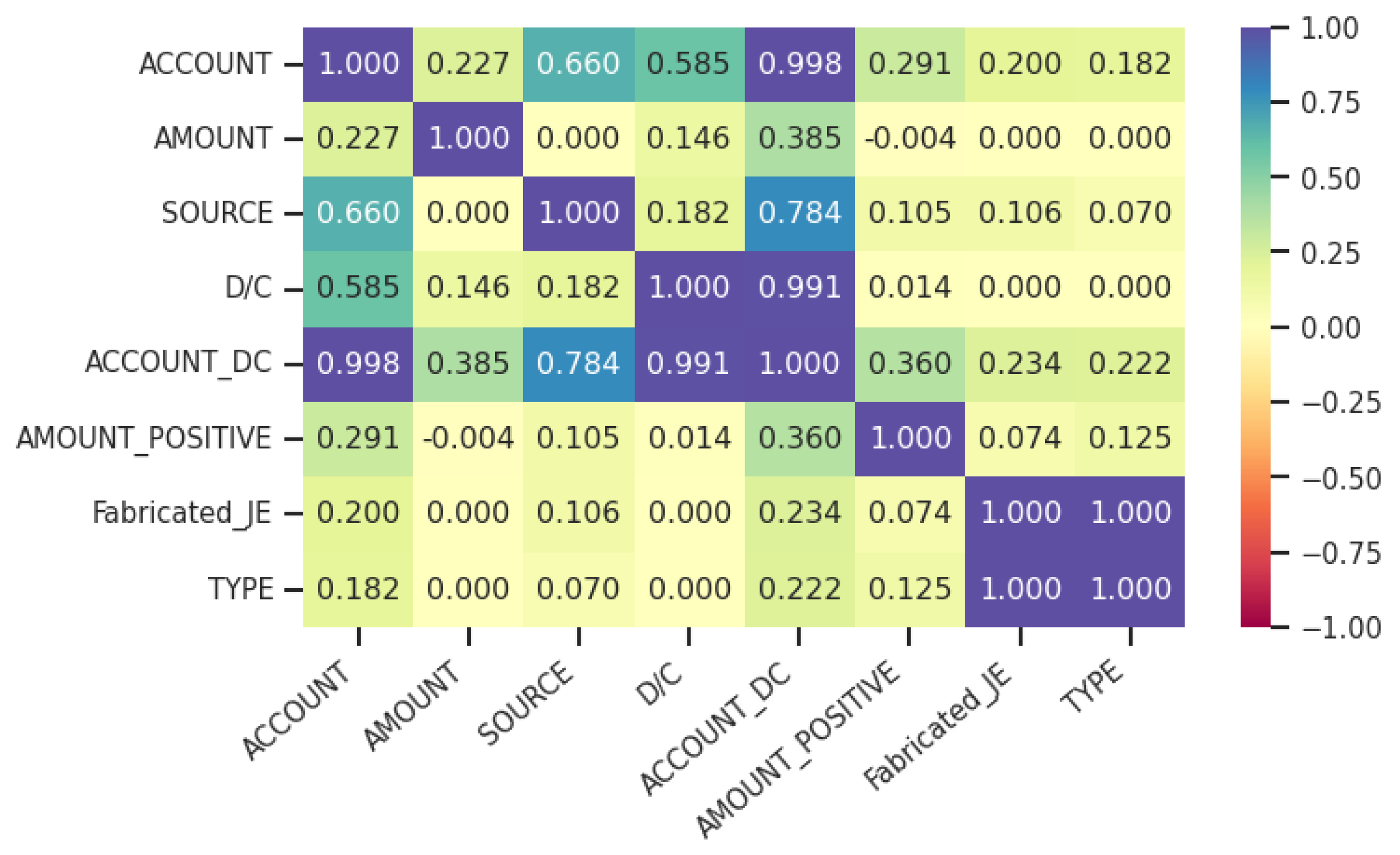
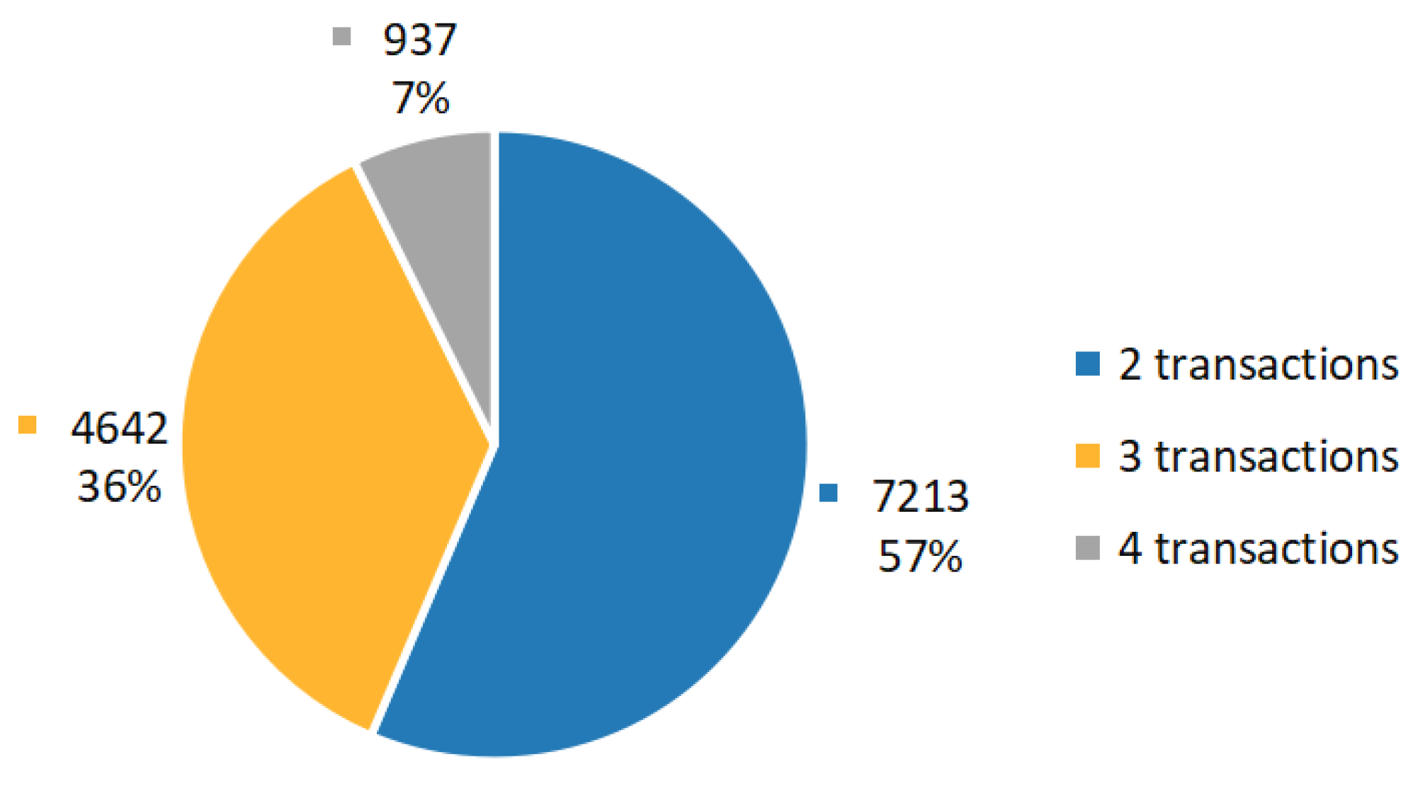
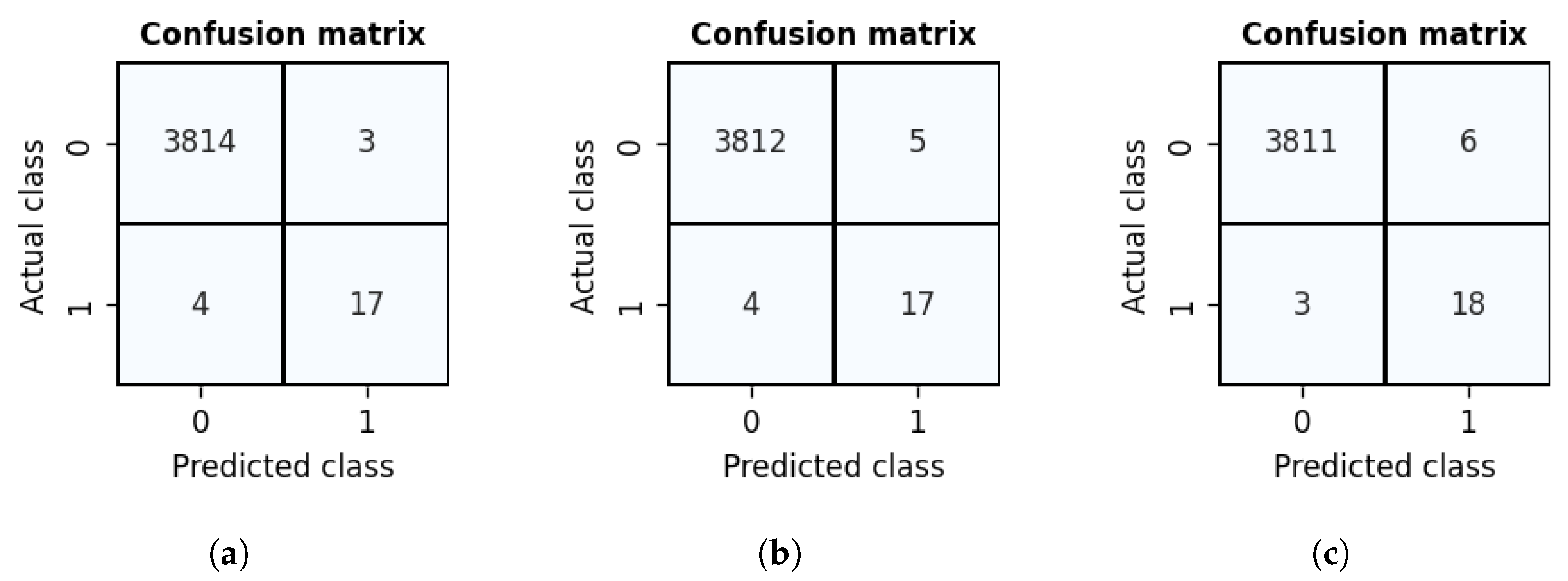
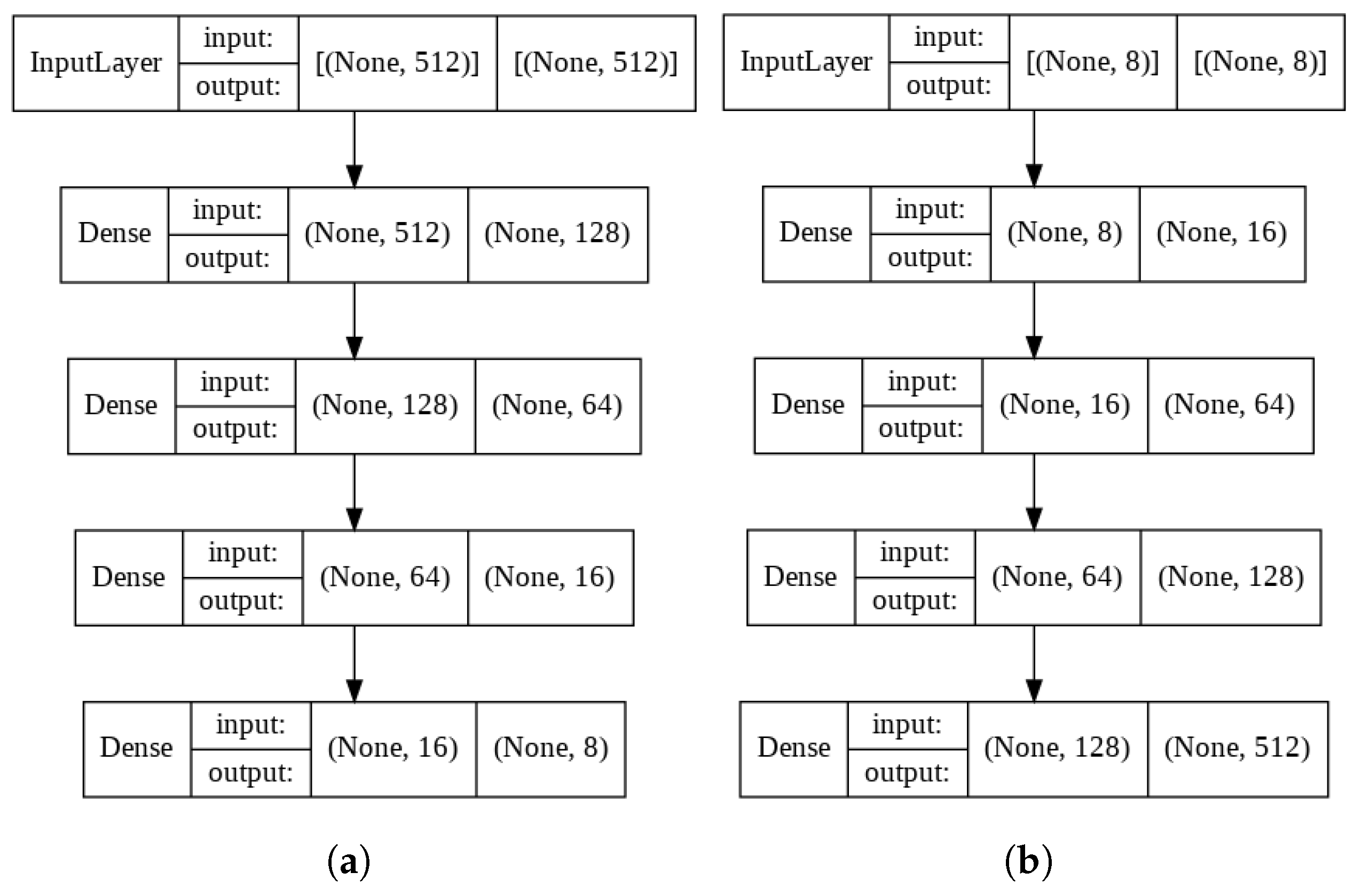
Table 1.
Anonymized data sample.
| JE_NO | EFF_DATE | ACCOUNT | AMOUNT | SOURCE | COMPANY | FY | Fabricated_JE | TYPE |
|---|---|---|---|---|---|---|---|---|
| A-111 | 2019-07-07 | 1930 | 10,512.00 | C | 44 | 2018-09-01–2019-08-31 | 0 | 0 |
| A-111 | 2019-07-07 | 1510 | −10,512.00 | C | 44 | 2018-09-01–2019-08-31 | 0 | 0 |
| B-111 | 2019-06-10 | 2330 | −2374.00 | E | 55 | 2018-07-01–2019-06-30 | 0 | 0 |
| B-111 | 2019-06-10 | 2440 | 2374.00 | E | 55 | 2018-07-01–2019-06-30 | 0 | 0 |
Table 2.
Dataset columns with data types.
| N | Column Name | Column Type |
|---|---|---|
| 0 | JE_NO | string |
| 1 | EFF_DATE | datetime |
| 2 | ACCOUNT | string |
| 3 | AMOUNT | float |
| 4 | SOURCE | string |
| 5 | COMPANY | string |
| 6 | FY | string |
| 7 | Fabricated_JE | string |
| 8 | TYPE | string |
Table 3.
Label counts on a transaction level.
| Label | Count |
|---|---|
| Normal data | 31,952 |
| Anomaly type 1 | 22 |
| Anomaly type 7 | 20 |
| Anomaly type 3 | 20 |
| Anomaly type 4 | 18 |
| Anomaly type 6 | 18 |
| Anomaly type 5 | 18 |
| Anomaly type 8 | 18 |
| Anomaly type 2 | 14 |
Table 4.
Non-anomaly and anomaly transaction counts.
| Label | Count |
|---|---|
| Normal data | 31,952 |
| Anomaly | 148 |
Table 5.
Description of introduced anomaly types.
| No. | Description |
|---|---|
| 1 | Classic mistake. Account that should not be combined with VAT. |
| 2 | Withdrawal cash to your private account and finance it by getting VAT back. Zero game for company, win for yourself. |
| 3 | Invoice with only VAT. Insurance which should be cost only (no VAT) has been recorded as only VAT. |
| 4 | Decreasing cost and getting VAT back. Improves margins and provides cash. |
| 5 | Increasing revenue and getting VAT back. Improve top line, margins and provides cash. |
| 6 | Inflating revenue, recording manual revenue and cost. |
| 7 | Fake revenue followed by clearing the invoice against account 4010 to make it look as if the invoice were paid, using the client payment process. |
| 8 | Double entry of supplier invoice, followed by recording it as being paid by creating revenue instead of reversing the invoice. |
Table 6.
Unique value counts for categorical columns.
| Column Name | Unique Count |
|---|---|
| JE_NO | 5105 |
| EFF_DATE | 1558 |
| ACCOUNT | 426 |
| SOURCE | 7 |
| COMPANY | 9 |
| FY | 18 |
| Fabricated_JE | 2 |
| TYPE | 9 |
Table 7.
Selected features for journal entry encoding.
| ACCOUNT | AMOUNT | SOURCE | D/C | ACCOUNT_DC | AMOUNT_POSITIVE |
|---|---|---|---|---|---|
| ✓ | ✓ |
Table 8.
Logistic regression model classification report.
| Precision | Recall | F1-Score | Support | |
|---|---|---|---|---|
| 0 | 1.00 | 0.98 | 0.99 | 3817 |
| 1 | 0.21 | 0.90 | 0.35 | 21 |
| accuracy | 0.98 | 3838 | ||
| macro avg | 0.61 | 0.94 | 0.67 | 3838 |
| weighted avg | 1.00 | 0.98 | 0.99 | 3838 |
Table 9.
Undiscovered anomaly types by logistic regression model.
| ID | Fabricated_JE | TYPE | y_Pred |
|---|---|---|---|
| 11410 | 1 | 8 | 0 |
| 11704 | 1 | 8 | 0 |
Table 10.
SVM model classification report.
| Precision | Recall | F1-Score | Support | |
|---|---|---|---|---|
| 0 | 1.00 | 0.98 | 0.99 | 3817 |
| 1 | 0.19 | 0.95 | 0.32 | 21 |
| accuracy | 0.98 | 3838 | ||
| macro avg | 0.60 | 0.97 | 0.65 | 3838 |
| weighted avg | 1.00 | 0.98 | 0.98 | 3838 |
Table 11.
Undiscovered anomaly types by SVM model.
| ID | Fabricated_JE | TYPE | y_Pred |
|---|---|---|---|
| 11410 | 1 | 8 | 0 |
Table 12.
Decision tree model classification report.
| Precision | Recall | F1-Score | Support | |
|---|---|---|---|---|
| 0 | 1.00 | 0.97 | 0.99 | 3817 |
| 1 | 0.16 | 1.00 | 0.28 | 21 |
| accuracy | 0.97 | 3838 | ||
| macro avg | 0.58 | 0.99 | 0.63 | 3838 |
| weighted avg | 1.00 | 0.97 | 0.98 | 3838 |
Table 13.
Random forest model classification report.
| Precision | Recall | F1-Score | Support | |
|---|---|---|---|---|
| 0 | 1.00 | 0.99 | 0.99 | 3817 |
| 1 | 0.27 | 1.00 | 0.42 | 21 |
| accuracy | 0.99 | 3838 | ||
| macro avg | 0.63 | 0.99 | 0.71 | 3838 |
| weighted avg | 1.00 | 0.99 | 0.99 | 3838 |
Table 14.
KNN model classification report.
| Precision | Recall | F1-Score | Support | |
|---|---|---|---|---|
| 0 | 1.00 | 1.00 | 1.00 | 3817 |
| 1 | 0.83 | 0.71 | 0.77 | 21 |
| accuracy | 1.00 | 3838 | ||
| macro avg | 0.92 | 0.86 | 0.88 | 3838 |
| weighted avg | 1.00 | 1.00 | 1.00 | 3838 |
Table 15.
Undiscovered anomaly types by KNN model.
| ID | Fabricated_JE | TYPE | y_Pred |
|---|---|---|---|
| 517 | 1 | 6 | 0 |
| 867 | 1 | 6 | 0 |
| 11410 | 1 | 8 | 0 |
| 11704 | 1 | 8 | 0 |
| 9494 | 1 | 8 | 0 |
| 603 | 1 | 1 | 0 |
Table 16.
Naïve Bayes model classification report.
| Precision | Recall | F1-Score | Support | |
|---|---|---|---|---|
| 0 | 1.00 | 1.00 | 1.00 | 3817 |
| 1 | 1.00 | 0.19 | 0.32 | 21 |
| accuracy | 1.00 | 3838 | ||
| macro avg | 1.00 | 0.60 | 0.66 | 3838 |
| weighted avg | 1.00 | 1.00 | 0.99 | 3838 |
Table 17.
Recall avg macro performance for three neural network models.
| Model No. | Model | No. of Hidden Layers | Recall Avg Macro |
|---|---|---|---|
| 1 (a) | Vanilla ANN | 1 | 0.9043 |
| 2 (b) | DNN1 | 2 | 0.9041 |
| 3 (c) | DNN2 | 3 | 0.9277 |
Table 18.
Supervised models’ evaluation comparison.
| No. | Algorithm | TN | FN | FP | TP | Recall Avg Macro |
|---|---|---|---|---|---|---|
| 1 | Logistic Regression | 3747 | 2 | 70 | 19 | 0.9432 |
| 2 | Support Vector Machines | 3732 | 1 | 85 | 20 | 0.9650 |
| 3 | Decision Tree | 3710 | 0 | 107 | 21 | 0.9859 |
| 4 | Random Forest | 3760 | 0 | 57 | 21 | 0.9925 |
| 5 | K-Nearest Neighbour | 3814 | 6 | 3 | 15 | 0.8567 |
| 6 | Naïve Bayes | 3817 | 17 | 0 | 4 | 0.5952 |
| 7 | Deep Neural Network | 3811 | 3 | 6 | 18 | 0.9277 |
Table 19.
Unsupervised models’ evaluation comparison.
| No. | Algorithm | TN | FN | FP | TP | Recall Avg Macro | Anom.% |
|---|---|---|---|---|---|---|---|
| 1 | Isolation Forest | 11,592 | 0 | 1130 | 70 | 0.9555 | 9.38 |
| 2 | Autoencoder | 11,301 | 0 | 1421 | 70 | 0.9441 | 11.65 |
Publisher’s Note: MDPI stays neutral with regard to jurisdictional claims in published maps and institutional affiliations. |
© 2022 by the authors. Licensee MDPI, Basel, Switzerland. This article is an open access article distributed under the terms and conditions of the Creative Commons Attribution (CC BY) license (https://creativecommons.org/licenses/by/4.0/).
Share and Cite
MDPI and ACS Style
Bakumenko, A.; Elragal, A. Detecting Anomalies in Financial Data Using Machine Learning Algorithms. Systems 2022, 10, 130. https://doi.org/10.3390/systems10050130
AMA Style
Bakumenko A, Elragal A. Detecting Anomalies in Financial Data Using Machine Learning Algorithms. Systems. 2022; 10(5):130. https://doi.org/10.3390/systems10050130
Chicago/Turabian StyleBakumenko, Alexander, and Ahmed Elragal. 2022. "Detecting Anomalies in Financial Data Using Machine Learning Algorithms" Systems 10, no. 5: 130. https://doi.org/10.3390/systems10050130
Note that from the first issue of 2016, this journal uses article numbers instead of page numbers. See further details here.