
Resilient Network Design: Disjoint Shortest Path Problem for Power Transmission Application
1
Department of Mathematics and Statistics, University of Calgary, Calgary, AB T2N 1N4, Canada
2
School of Management, Zhejiang University, Hangzhou 310058, China
3
Gurobi Optimization, LLC, Beaverton, OR 97008-7105, USA
*
Author to whom correspondence should be addressed.
Systems 2024, 12(4), 117; https://doi.org/10.3390/systems12040117
Submission received: 10 December 2023
/
Revised: 12 March 2024
/
Accepted: 27 March 2024
/
Published: 31 March 2024
(This article belongs to the Special Issue Developing Resilient Systems: Engineering Solutions for a Changing World)
Abstract
:Path redundancy is essential for safety and reliability in many real-world routing problems, such as the design of networks for power transmission, transportation, etc. These problems are typically posed to find the shortest path on a weighted graph. For the shortest path with path redundancy, particularly in the Disjoint Shortest 2-Path (DS2P) problem, two disjoint paths are desired such that the combined weight of the two paths is minimized while a minimum distance path separation is maintained. The conventional formulation of the above requires a large-scale mixed-integer programming (MIP) model. However, this approach is practically intractable due to the model’s complexity and extremely long run-time. We demonstrate why DS2P is NP-complete and propose an efficient heuristic to find an approximate solution to the problem in a much shorter time frame. We demonstrate the approach on a realistic dataset for power transmission routing, integrating the computational methodology with a visualization interface using Google Maps. The resulting prototype software is freely available through GitHub and can be deployed on a cloud platform, such as Amazon AWS.
1. Introduction
Catastrophic changes in operational and natural environments present huge risks and uncertainties in supply chains. A common solution to make a system more resilient to such catastrophic changes is to build in some redundancy. Redundancy in power transmission lines as a protective measure is recommended by the IEEE Power System Relaying and Control Committee (PSRC) and is regulated by the North American Electric Reliability Corporation (NERC). According to [1], the physical separation of designated groups in a redundancy protection system should be maintained to ensure failure resilience in case of catastrophic events. The recommendation of physical separation is a part of bulk power system protection criteria in some North American regional electricity organizations. A natural question arises: how can we add the necessary level of redundancy for the least possible cost?
Transmission line routing is a classical applied optimization problem. Numerous approaches, such as the raster-based GIS approach, genetic algorithms, and graph-theoretical methods, have been proposed to identify the shortest or least-cost path or paths over a given locale, demonstrating varying degrees of success largely dependent on the complexity of the underlying model. Our work is motivated by a practical question—optimal transmission powerline routing (with redundancy constraint)—as further described in Section 1.2.
A common abstraction of the routing problem is to model the system as a graph. Many utility metrics are reduced to graph properties, such as the shortest path between two vertices, etc. A basic illustration of a classical shortest (here, least-cost) path is given in Figure 1, where the path is depicted in red.
The effective solution techniques for the shortest path problem stand out as a set of notable achievements of classical Operations Research stemming from the original work of Dijkstra in the late 1950s [2]. To date, the shortest path problem has found many applications in network design, GPS routing, etc. Although the shortest path has been shown to be computationally easy, some of its innocent-looking variants present incomparable challenges.
We study a variant of the shortest path problem, which we refer to as the Disjoint Shortest 2-path Problem (DS2P), in which two disjoint paths need to be determined instead of one, and in addition, the paths have to conform to some minimum-distance constraints. By distance constraints, we mean that the two paths have to be at least a certain distance apart from each other. The DS2P problem variant is poorly understood.
Our main contribution is the proposal of a novel method to account for distance constraints that, under certain assumptions, guarantee optimal two-path recovery in a very modest run-time. If the assumptions are not met, our method can be regarded as a heuristic. The method is based on a geometric embedding of a two-path problem in a higher-dimensional graph, followed by the shortest-path computation. In the embedding model, hard geometric constraints are converted to the graph’s connectivity with the associated cost structure. The computational run-time requirements to recover an optimal set of two geometrically distinct paths grow moderately as compared to all the other known alternatives, resulting in an efficient numerical procedure. Along the way, we classify the hardness of DS2P and give an exact 0-1 integer programming formulation of the two-path problem, and we demonstrate the comparative advantages of our embedding approach. Our method can be generalized to accommodate distinct origin–destination pairs and more complicated geometric constraints.
Shortest path routing is often one of the most important aspects of infrastructure projects such as roads, pipelines, or power transmission lines. Conventional ways to find the shortest/most economical paths mostly rely on survey data and available maps. Other digital technologies like remote sensing, image processing, drone surveys, geographical information systems (GIS), etc., have made the task less daunting and more precise in terms of data availability. Due to these technologies, huge amounts of data are, in principle, available to facilitate good decision-making. However, the challenge lies in how to use the available information effectively. We illustrate how the novel DS2P methodology can be embedded into a data-driven decision-making cycle for optimal powerline routing, including integration with Google Maps and cloud deployment.
The manuscript is organized as follows: in Section 2, we first formulate the problem on a graph and then present a corresponding 0-1 MIP model formulation; in Section 3, we discuss some basic properties of the exact models, including the complexity of the graph-based model and the linear programming relaxation of the 0-1 programming model; in Section 4, we introduce our novel approximation scheme; and in Section 5, we further illustrate how the new approach can be used for practical data-driven decision-making.
1.1. Literature Review and Related Works
In many applications, a necessity arises to determine a set of alternative paths between some source–sink pair. For example, a multi-path concept was applied for network robustness in the context of transit design in [3]. In [4], the authors studied a related path diversification problem with an application to a transportation network. The authors presented an experimental approach reliant on network and path penalization and evaluated various trade-offs for a Washington DC area case study. An interesting approach to road path diversification (without geometric constraints) is presented in [5] and relies on a physical analogy to electric power flow and its formal analysis. In [6], the authors studied the survivability of low-cost communication networks. Some of the proposed models fall within the domain of so-called bilevel programming, while others pursue a graph-theoretic approach.
Transmission line routing and planning have long drawn attention as an application of the shortest path problem as well; see, for example, [7,8]. Much work in the literature focuses on expansion planning, where the routes are well documented by transmission owners or regulators [9]. Classical engineering reliability aspects of power systems are already well covered in the literature; for example, see [10,11]. In [12], the authors considered the question of re-configuring the power network following a natural disaster, including better locations for transformers and maintenance holes in the grid, proposing a hybrid optimization-based heuristic approach. The optimal placement of the new transmission lines corresponds to the topological design of a very specialized unorthodox “supply chain”, where multiple power lines serve to increase the system’s resilience to catastrophic failures.
The shortest-path application in transmission line routing has drawn collaborative attention from industry and academia. Ref. [13] used a genetic algorithm and an improved Artificial Bee Colony algorithm in combination with a total weight surface raster map to find the single shortest path. ArcGis is a product of ESRI and is extensively used for preparing GIS-related input in the form of a pixelated dataset called a raster, with each cell having a value. These datasets can be used as cost metrics for finding the shortest paths. Ref. [14] used dynamic programming (DP) with GIS to create a raster cost map, which includes geographic as well as non-geographic costs, to give a DP-embedded GIS-based grid in which each cell represents the minimum cost from the origin. The economic corridor for transmission line laying is typically defined within a boundary region that allows some deviation from the optimal route for feasibility. Ref. [15] discusses the drawbacks of raster-based shortest-path solutions, mainly attributed to the discretization of the continuous space. A geometric distortion associated with the rectangular aspect of rasters is discussed in [16]. Ref. [17] suggests two types of geometric distortions: elongation and deviation distortions. Ref. [18] defines elongation as the ratio between the costs of the least-cost path (LCP) and the true LCP. The deviation distortion corresponds to the absolute difference in location between the LCP and the true LCP [19]. Further, ref. [18] introduced a third type, proximity distortion, which is caused by ignoring the effects of neighboring cells. There are alternative methods like vector-based graphs and GA-based approaches to overcome the pitfalls of raster-based methods. Ref. [15] also points out the drawbacks of a GA, which mainly results in the probabilistic heuristic nature of the solution. Thus, the raster-based approach to the LCP is preferred over the GA approach for being exact in identifying the LCP.
To determine the single shortest (or least-cost) path between any two nodes in the graph, besides the classical Dijkstra algorithm [2], other efficient and specialized algorithms exist, such as the Bellman–Ford algorithm [20,21], Fredman and Tarjan’s algorithm [22], etc. Similarly, there are methods to efficiently compute the shortest paths between all pairs of vertices, e.g., the Floyd–Warshall algorithm [23,24]. These algorithms are very computationally efficient and allow one to find the shortest path for very large (nonnegatively weighted) sparse graphs with relative ease. Depending on the algorithm, one can complete this task within a constant multiple of either or arithmetic operations, where and denote the number of edges and vertices in the graph.
One well-studied extension of the classical shortest path problem is the so-called K shortest path routing problem. Here, the aim is to find not only one single shortest path but also the other paths in a non-decreasing order of cost. Due to its importance, the K shortest path problem is well studied. For brevity, we give only two entry points to this field of research, namely, [25,26], where polynomial-time algorithms were given. There are also versions of algorithms determining the existence of -disjoint paths between distinct pairs of vertices , … in a given graph . This variant of the -disjoint path problem has also been extensively studied as well, and again, for brevity, we only cite [27] here, where polynomial algorithms are proposed. Another notable extension is attributed to Suurbale’s algorithm [28], which allows us to find a min-cost pair of disjoint paths between the two vertices in a nonnegatively weighted directed graph. A good and updated brief survey of disjoint paths in networks can be found in [29].
Unlike the classical single shortest path problem, or the above K shortest path routing problem or the -disjoint path problem, few practical and well-understood approaches exist for the 2-path variant with “geometric” constraints, applicable to large networks. An example of geometric constraints is a situation where paths are further required to be separated by some minimum distance. Although the latter problem has many potential applications, to our knowledge, no efficient general-purpose method exists for DS2P where the user can specify such a geometric constraint. In [30], the authors consider a very closely related minimum-cost pair in the D-geodiverse paths problem. Our DS2P problem is slightly more general; it can be posed on an abstract graph and is not reliant on a specific Euclidean embedding. The authors explored a MIP-based approach for models posed over relatively small graphs, particularly featuring two (communication) network topologies: Germany50 with 50 nodes and 88 links and CORONET CONUS with 75 nodes and 99 links. The main difference between our work and [30] is the target size of the network: MIP works well for small topologies, while for medium to large networks with thousands of nodes or more, we quickly hit the computational wall, and other solution techniques are required. Similarly, in [31], the authors propose an extension of the D-geodiverse problem to paths, relying on a similar MIP approach and, hence, subject to similar computational limitations. In contrast, for larger networks, mostly heuristic methods lacking rigorous analysis have been proposed. For instance, when two paths are desired, a manual search is usually performed on a set of K-disjoint paths, instead of systematically recovering the cheapest pair of paths. Unlike the identification of a single least-cost path, the case of the DS2P, where we need to introduce separation constraints between the paths, does not have commercially available software packages. In a typical powerline application, the size of a graph representing a possible network topology is large (thousands and even millions of nodes alone). As a consequence of using unproven heuristics, one may end up with sub-optimal solutions, which could result in a large unrealized socio-economic potential.
1.2. Motivational Example
The northeast region of Alberta, Canada, is an area with the highest growth in electricity demand across the province. Energy and oil sand industries in the Fort McMurray area constitute a large portion of the current and future electricity demand. On the other hand, a large amount of hydro energy is available in the Slave River basin, which is located at the northern border of the Alberta province. The problem is how to transmit electricity to the Fort McMurray area. The northern region has a very sparse population, and most of the area is covered with forests and ice; there is almost no human development in the area. Hydro-generated power has to be transmitted via power lines to substations in the vicinity of the facilities in Fort McMurray. Through this, it is possible to bring green energy to energy-intensive operations and contribute to greenhouse gas reduction plans.
There are many geographical, environmental, economic, human footprint, and other considerations in the region. To quantify these, the regional map can be discretized using a desired resolution, and each cell in the grid can be assigned a representative “weight” corresponding to a power line transitioning through the cell. The resulting color-wash map is presented in Figure 2, with brighter-red colors corresponding to more expensive regions in terms of the anticipated construction cost. The detailed map is divided into 311-by-244 cells of 1 × 1 km cell size resolution. The representative construction costs for each cell were determined in collaboration with the Alberta Electric System Operator using the blend of automated rasterization and a manual process. The costs consider topographical features, accessibility, and other considerations. Two dark-red areas correspond to the forbidden zones where large water bodies are located and the cost of transmission line construction may as well be assumed to be infinite.
The objective is to find the optimal route or corridor for the power lines in northeastern Alberta. A hypothetical northeastern Alberta powerline topology is presented in Figure 3, with a star depicting the generator facility and a circle depicting the receiver station. When designing a power transmission line between the generating facility and the consumer node, a company may be legally required to build not just one but two redundant power lines, distanced from one another by some minimum safety margin, so that if one of the lines goes down due to an accident, there is still a high probability of power being delivered to the destination via the second back-up line.
Thus, we aim to find two separate corridors for transmission lines going from the power plant to the substation. Because of the specific reliability standards, these two lines must be separated by a distance of at least 50 km or, equivalently, must be 50-unit cells apart. The latter problem may be abstracted to solving an instance of DS2P—finding the two shortest paths on a graph subject to a geometric distance constraint with vertices representing cell centers and edges representing the cost of transitioning from any one cell to another.
Similar to the powerline design problem, a distance-constrained 2-path problem naturally arises in road construction, high-capacity fiber-optic cable network design for telecom, and GPS navigation. We expect an efficient solution approach to DS2P to benefit these application areas as well.
2. Problem Formulations
In this section, we propose two formulations of DS2P. The first formulation approaches the problem from a graph-theoretic viewpoint. The second formulation is based on so-called mixed-integer programming, or more specifically, 0-1 integer programming. Both formulations may be regarded as general models in the sense that distance constraints can take more exotic and abstract forms. However, since this work is motivated by a practical problem, we pay the most attention to the Euclidean or counting metric measuring the distance. The first formulation is used to establish a hardness result for the corresponding variant of DS2P. The second model closely relates to the well-known min-cost flow problem and provides a convenient computational baseline for comparison; see Section 5.3.1.
2.1. Graph-Based Problem Formulation
For simplicity, from now on, we assume that we are dealing with a finite, directed, weighted graph with vertices indexed by . Let represent the edge going from vertex i to j, with the associated weight . Note that we work with directed graphs and, generally speaking, may have . We introduce a special pair of vertices, where the source is denoted by s and the sink by t. A path from the vertex u to v is an ordered collection of vertices so that for every consecutive pair , there exists an edge ; we say that the path has the length k in accordance with the number of edges used, counting possible multiplicities. An edge is a path of length 1. Between any two vertices in a graph, there may be no path at all, a unique path, or a set of alternative paths, depending on the graph’s configuration. The path has a cumulative cost .
We proceed with stating the classical (single) shortest path problem.
Problem 1.
Given a graph , with terminal vertices , find a path so that its cumulative cost is minimized, where , .
To define the 2-path variant with distance constraints between the paths, it is useful to introduce the notions of reachability and neighborhood.
Definition 1.
The vertex u is Δ-reachable from v if there exists a -path of length Δ or less.
In our setup, reachability is used to determine the distance between the paths and thus serves largely as a surrogate for the geometric distance. To this end, since the Euclidean distance is symmetric, when referring to u as -reachable from v, we understand this in the context of using the underlying undirected version of the graph obtained by replacing every edge of with a bi-directional edge.
Definition 2.
A Δ-neighborhood of a vertex v denoted by is a subset of such that whenever u is Δ-reachable from v.
- The main reason to introduce the notion of a neighborhood is that the distance constraint has to be relaxed for the edges near the source and the sink; otherwise, the model ceases to be meaningful and becomes infeasible. Now, we are in a position to state our first and rather more abstract variant of DS2P.
Problem 2.
Given a directed graph , a source , a sink , and a fixed distance threshold Δ, find two paths from s to t, defining them by and , such that
- (i)
- The two paths are at least Δ-distance apart with respect to the counting (edge) metric, i.e.,for alland allthe vertex v is not -reachable from ;
- (ii)
- The total cost is minimized among all possible paths satisfying (i).
For simplicity, we can take and in the above, while, generally, the neighborhoods of the source and sink can be further modified if required; see Figure 4a.
Generally, in what follows, when we want to emphasize graph nodes, they are depicted with larger figure elements, e.g., labeled circles. However, when we want to emphasize edges and cost structure, the nodes are often depicted as dots, while a color-wash scheme, like in Figure 2, is used for the edges.
An example of a directed graph is shown in Figure 4b with source at 1 and sink at 6. Since is non-planar, using the Euclidean distance between vertices to capture the distance between the paths ceases to make sense. However, the statement of DS2P with and still makes sense, with the solution given by and . Thus, the use of a more abstract counting metric fits general graphs—planar or non-planar.
The scenario where , , and is very important, and its significance will be seen when DS2P complexity is discussed.
2.2. The 0-1 Integer Programming Model
As we have mentioned, the bulk of the 0-1 integer programming model relates to the min-cost flow formulation of the shortest path problem. We introduce the min-cost flow model first and then propose the 0-1 integer programming formulation for DS2P.
A flow over an edge is a real number assigned to the edge. Intuitively, this can be thought of as the quantity of goods carried on a road segment, or the amount of water flowing through a pipe. The min-cost flow problem is the central object of study in almost every book on network flows. Besides its theoretical importance, problems that are modeled as min-cost flow constantly arise in industries, including manufacturing, communication, transportation, and so on. The min-cost flow problem is typically defined over a capacitated network; that is, in addition to the edge cost , there is a capacity for each edge , signifying that the flow along -edge cannot exceed . Now, the min-cost flow model is given as follows (see, for instance, [32], p. 296).
Problem 3.
With each vertex , we associate a number , which indicates whether the vertex is a supply or a demand node, depending on whether or , respectively. The min-cost flow problem solves the following linear programming instance, where represents the flow along the -edge:
In its generic form, the min-cost flow problem allows for fractional optimal flow values. However, under certain assumptions, it yields integer flows only. Specifically, when all the capacities and are integers, we have integer optimal flow values . By making clever choices for and , we can model many situations, including the shortest path problem.
First, observe that the shortest path problem may be formulated as the following 0-1 integer programming problem:
Problem 4.
The binary variables are used to indicate whether the -edge is used in the construction of the shortest path—set —or not—set . The affine constraint guarantees the flow conservation. The source s has one unit of flow out, and the sink t has one unit of flow in. All the other vertices always have zero-net flow since only one unit of flow is allowed to go in and out. Next, we note that, due to the integrality property, the binary variables may be replaced with continuous capacitated variables, , , thus giving us an instance of min-cost flow.
Similarly, we can easily formulate the DS2P problem by adding one more flow corresponding to the y-variables along with the required minimum-distance constraint , where measures the distance between the vertices (or the edges), and is the required threshold.
Problem 5.
Similarly to for the first path, binary variables are used to indicate whether the edge belongs to the second path or not. By restricting the cumulative flow through the -edge to be no greater than 1 (see the fourth group of affine inequality constraints above), we permit only one path within close proximity to the other. We intentionally do not specify the distance function to keep the model as flexible as possible. In particular, can be chosen to represent either the counting reachability metric or the Euclidean distance based on the graph’s embedding.
The above model corresponds to solving an instance of 0-1 programming, while MIP instances in general are notoriously difficult. A natural question arises: can we simply relax the binary restriction on the variables into linear inequalities, as was the case for a single shortest-path formulation? We address the hardness classification of DS2P next, before addressing the former.
3. Basic Properties of DS2P Models
3.1. Graph-Based Problem Complexity
We show that for , the decision version of DS2P is NP-hard by relating the problem to the so-called 3SAT problem. In contrast, when , DS2P is easy and can be reduced to the standard shortest path. Since, in practice, we are most likely to be interested in more than vertex-disjoint paths, that is, cases where , this turns our prospects of solving DS2P over general graphs quite bleak.
The 3SAT problem is an important example of an NP-complete problem. We review its statement next, along with some auxiliary definitions.
Definition 3.
A Boolean expression consists of binary variables (0 means false while 1 means true), three operations—AND (i.e., conjunction, denoted by ∧), OR (i.e., disjunction, denoted by ∨), and NOT (i.e., negation, denoted by a bar above the variable)—and parentheses.
Definition 4.
The Boolean satisfiability problem, abbreviated as SAT, is the problem of determining whether an assignment exists to satisfy a given Boolean expression. When there exists such an assignment, it is called a true assignment, and the given Boolean expression is satisfiable.
For example, , , and with resulting negations , etc., is a true assignment for the Boolean expression , and consequently, this Boolean expression is satisfiable.
To be consistent with terms in Computer Science, we introduce the following jargon: a literal is either a variable, then called positive literal, or the negation of a variable, then called negative literal; a clause is a disjunction of literals, or a single literal. The 3SAT problem is a type of Boolean satisfiability problem with a specific structure, namely, that each clause contains exactly three literals. For example, finding a true assignment for is a 3SAT problem.
Theorem 1
([33] p. 48). The 3SAT problem is NP-complete.
Interestingly, the behavior of DS2P varies drastically with the desired distance between the paths. Specifically, when , the problem is very easy, while for , DS2P becomes very hard. We proceed to illustrate this phenomenon in detail.
Setting leads to the vertex-disjoint shortest path problem. Polynomial algorithms are given for the vertex-disjoint shortest path problem in undirected graphs with positive weights in [27,34]. The corresponding digraph can be modified so that the problem fits the min-cost flow model [28]. We illustrate the latter modification procedure with an example in Figure 5, where the solid lines have cost 0 and the dashed lines have cost 1.
Suppose we want to find two vertex-disjoint shortest paths from node-1 to node-4. If we simply implement the min-cost flow model to deliver two units of flow in total—derived from Problem 4, with integrality relaxed to and the non-zero RHS replaced by —we will obtain {1,2,3,4} and {1,3,5,4}, whose total cost is zero. However, these two paths have a common vertex: node-3. The modification in Figure 5 guarantees that every node is visited only once, since the edge can only be used once. The min-cost flow model has the property of having integer flow, and since the corresponding LP problem is in P, we conclude that the problem with is in P as well.
When considering DS2P and related instances, it is worthwhile to mention that the following problem (stated in [27]) is NP-complete.
Problem 6.
Given a graph with positive edge weights and two pairs of vertices , , find whether there exist two disjoint (edge-disjoint or vertex-disjoint) paths from to and from to such that is the shortest path.
Inspired by the reduction technique of Problem 6 in [27], we have the following theorem:
Theorem 2.
Let and .
If , then DS2P is in P.
If , then DS2P is in NP-hard.
Proof.
Denote the number of clauses and the number of literals in the expression by m and n, respectively. For each clause , we construct a sub-graph , and for each pair of literals and , we construct a sub-graph , as shown in Figure 6. has nine edges, and the three middle ones represent the corresponding literals , , and . has two sides: the left side consists of the edges of , and the right side consists of the edges of . Denote the times that each literal appears in all s by , and let the length of both sides of be so that both sides have edges of and , respectively. This construction process is a polynomial-time transformation.
Connect each sequentially by coinciding one’s last vertex with the next one’s first vertex, and repeat the same process for each . Then, connect each pair of vertices that are incident with the edge of the literal in s to the ones in s incident with the edge of with dashed lines, respectively and sequentially. We use solid lines to connect the source s to the initial points and of sub-graphs A and B, respectively, and connect the sink t to the ending points and as well, and we use dashed lines to connect to and to . Set the weight of all the solid lines to 1 and the weight of all the dashed lines to . For example, Figure 7 is constructed for , and Figure 8 is constructed for .
We claim that finding two disjoint shortest paths subject to the distance constraint from s to t in Figure 7 is equivalent to solving the 3SAT problem . Note that Figure 7 has the following properties:
- 1.
- DS2P is always feasible: there are always two paths satisfying all the constraints, that is, and , whose total cost is .
- 2.
- Every variable admits a unique assignment: if the first path goes through the edge in , the second path cannot go through the edge in due to the distance constraint .
- 3.
- The DS2P optimum determines the satisfiability. For convenience, we denote the path that goes through sub-graphs s (or s) by A (or B) and otherwise by (or ), and by , we mean that, under the distance constraint, the two situations A and co-occur; that is, one of the two paths goes through all s, while the other does not go through all s. There are four scenarios:
- (a)
- , and then the least cost is ;
- (b)
- , and then the least cost is ;
- (c)
- , and then the least cost is ;
- (d)
- , and then the least cost is .
It is straightforward thatand Scenario (a) implies that the corresponding 3SAT problem has a true assignment.
In the example shown in Figure 7, there exist two such disjoint shortest paths:
(we allow for a slight abuse of notation in the above for the sake of brevity).
If we set all the literals in to be true, that is,
then , and we solve the 3SAT problem.
In the example shown in Figure 8, there do not exist two such paths with the total cost that satisfy the distance constraint. And it is not a coincidence that the corresponding 3SAT problem has no true assignment, meaning it is always false.
Considering these two examples together, we can see that, indeed, the outcome of solving a DS2P problem implies the satisfiability of its corresponding 3SAT expression. If the outcome shows that the cost equals , then it has a true assignment, which can be expressed by the path from to ; otherwise, the 3SAT expression is always false.
Graphs constructed for scenarios when can be regarded as subdivisions of the graph of the scenario when . This reduction applies regardless of whether the graph is directed or undirected; hence, for both types of graphs, the DS2P problem with is NP-hard. □
3.2. LP Relaxation of the DS2P 0-1 Programming Model
Recall that, in Section 2.2, we presented the 0-1 MIP formulation of the single shortest path problem. An additional and crucial property that makes this formulation so useful is the solution integrality of the respective LP relaxation. The latter feature of the min-cost flow re-formulation of the classical shortest path problem is commonly referred to as the Integrality Theorem ([32] p. 381).
Theorem 3.
If all edge capacities and supplies/demands of nodes are integers, the min-cost flow problem always has integer optimal min-cost flow values.
Thus, a reasonable question here is whether the LP relaxation of DS2P Formulation 5 has a similar favorable integrality property. Specifically, consider the following linear programming relaxation to be the MIP equivalent to Problem 5 (here, for convenience, we have added a spurious edge of capacity 2 between the sink and the source and forced a unit of flow throughout x and y variables).
Problem 7.
Unfortunately, the integrality of the LP relaxation solution is lost, as is illustrated in the next example.
Suppose we want to solve a DS2P problem for the uniform grid graph shown in Figure 9, where node-1 is the source, node-16 is the sink, all the solid edges have cost 1, and dashed edges have cost ∞. Clearly, we want the paths to go along the solid lines, as, otherwise, the total cost of the paths would be infinite. If we further require the Euclidean distance to be strictly bigger than , with the exception of vertices immediately adjacent to the source and sink, then there do not exist two such paths with finite cost, since the Euclidean distance between node-8 and node-9 is exactly . However, it can be easily verified that the LP relaxation may yield four fractional flows as a feasible solution:
A slight modification of this example, with the infinite edge cost replaced with large finite values, gives a situation where rounding these fractional solution values provides no additional useful information to construct an incumbent. In short, we believe that the MIP formulation has a fairly weak LP relaxation, which is often a good predictor that solving the MIP model (with a standard branch-and-bound approach) will be difficult.
We should also note that the cardinality of the distance constraints is expected to grow very rapidly for practical graphs representing physical path routing. So, we may indeed have a very hard and large instance of a 0-1 programming problem representing DS2P.
4. A Novel Approximation Scheme
It has been shown that the general version of DS2P is hard. Therefore, we make some simplifying assumptions, starting with graph topology, that, in turn, allow us to introduce an efficient heuristic approach. We focus on the minimum Euclidean separating distance between the path version of the problem, while one can easily translate what follows for the case of an edge-based counting metric between the paths.
4.1. Special “Diamond” Graph
From now on, we assume that the real-world (good) path connectivity can be well represented using a bi-connected directed diamond graph. In other words, we fix the path’s topology to those realizable over a diamond grid, assuming that such paths provide enough good options for selection from a practical point. From an explanation point of view, it is convenient to first describe a version of such a graph along with its particular 2D embedding.
Geometrically, the diamond graph corresponds to a uniform square K-by-K grid, with vertices located at the grid points and (diagonal downward) edges, with the source being the top-most and the sink being the bottom-most vertex; see Figure 10.
Using such a graph configuration is motivated by simplicity and the large computational advantages it provides. From a usability point of view, albeit restrictive, we also do not see this configuration as unreasonable. We expect that, in practice, such as in the case of our motivating example from Section 1.2, the cost data are obtained as a set of some sample values, e.g., a matrix of the representative cost per unit path length on a discretized regular grid superimposed over a geographical area of interest. Assuming that the majority of cost values are not dramatically different from cell to cell—possibly justified by the terrain being largely homogeneous—it is reasonable to expect that “good” paths mostly proceed in the direction from the start location toward the terminus (in our Figure 10, this is colinear to the z-axis) and do not contain large backward loops. In other words, if we have enough options to traverse the distance between the source and the sink, it is unlikely that making a backward loop will decrease the overall construction cost and become economical. The expansion of the diamond grid toward the middle as we traverse the z-axis allows for a wide range of possible path configurations, while as we approach the terminal nodes, it is reasonable to assume that the paths will narrow down toward the source and sink.
It is quite possible that, in the neighborhoods of the source and sink, where the minimum-distance constraints are not applicable, permitting more flexible path trajectories is of higher importance. In practical terms, we think of the source and sink as being in more confined sub-regions, e.g., due to urban development. Once we depart from the respective neighborhoods of the source and sink, the terrain becomes more homogeneous and less restrictive. To accommodate more flexibility in the vicinity of the terminal nodes, one can augment the diamond graph topology by replacing it with a truncated diamond graph and adding complete sub-graphs around the source and sink; see Section 5.2. Similarly, the graph embedding on the uniform Euclidean grid is applied out of convenience, while other embedding variants may also be considered, including non-grid-based embedding, and potentially represent more exotic path segments, e.g., the curvy path segments in Figure 11b.
It should also be noted that the bi-connected diamond graph can be used to emulate a higher degree of connectivity between the desired vertices. For instance, we can accommodate the addition of vertical edges by doubling the grid density and appropriately defining the new edge cost, as illustrated in Figure 11a. The dotted edges represent a prohibitively high cost—think ∞ or in excess of the sum total of the edge costs of the initial graph—and are priced as such to prevent the “spurious” paths from cutting through the middle of each cell; thicker solid edges have zero cost. The respective algorithmic modifications of our scheme are quite straightforward and are deferred to later subsections. Unless mentioned otherwise, here, we focus on a diamond graph for clarity.
To facilitate the explanation, we use three types of labels for the vertices of the diamond graph in Figure 10, which are in one-to-one correspondence with each other:
- corresponds to array-like indexing along the index axis;
- corresponds to vertex labeling by -coordinates in the given embedding;
- is a left-to-right and top-to-bottom vertex enumeration index.
For example, in the figure, corresponds to the source, and corresponds to the sink vertex. We have
and
with . Since, in some sense, the z-coordinate measures the path’s progress toward the sink, we will occasionally refer to the z-value as a level; see Figure 10.
As a reminder, our ultimate goal is to find the optimal pair of paths that are at least units apart. We believe that the computational advantages offered by the diamond graph topology outweigh the downsides of working with the restrictive graph class, at least in applications to a longer-range resilient electric power supply design.
4.2. Three-Dimensional Embedding
The main idea of our approach is to embed the distance-between-the-paths constraint within the graph structure itself, possibly by increasing the dimensionality of the embedding, rather than adding the distance constraints to a planar graph model representing a single path. Out of a planar diamond graph, we construct a 3D graph that represents two paths simultaneously, whose vertices and edges can be carefully chosen to approximate the minimum-distance requirement. To this end, we will use the horizontal distance between the paths as a surrogate for the minimum distance. In the case of using a uniform Euclidean grid for the path’s metric embedding, as per Figure 10, if the two paths are d units apart in the x-direction, the paths cannot be closer than to one another; see Figure 12. The distance approximation constant depends on the particular embedding chosen; e.g., think of stretching or compressing the grid in the z-direction. By picking a suitably large d, one can guarantee that the paths have a certain minimum distance in between. We also note that by increasing d, one may inadvertently make the search space unnecessarily restrictive. Thus, in practice, we may want to take a balanced approach when selecting a specific value of d. In what follows, we will illustrate that, due to our scheme being particularly efficient, such ad hoc decisions can be made in near real time.
We proceed to describe how the 3D graph is constructed in the pseudo-code below, using primarily Euclidean vertex labeling.
- Input:
- (2D) diamond graph corresponding to uniform grid along with edge cost , and minimum horizontal path distance threshold d.
- 0.
- Initialize% Populate the set of 3D vertices
- 1.
- for
- 2.
- if
- 3.
- set
- 4.
- else
- 5.
- for
- 6.
- for
- 7.
- if
- 8.
- set
- 9.
- for
- 10.
- set
- 11.
- if
- 12.
- set
- 13.
- else
- 14.
- for
- 15.
- for
- 16.
- if
- 17.
- set% Populate the set of 3D edges and respective edge cost
- 18.
- for
- 19.
- for all vertices
- 20.
- for all so that
- 21.
- if vertex
- 22.
- set
- 23.
- set
- 24.
- set edge cost
- Output:
- (3D) embedding graph with edge cost .
where
- for iterator = start_value:increment:end_value
- denotes a Matlab-like for-loop, while if increment is omitted, we increment by 1, and
- for all members in a set
- is used to iterate over the set, and
- % is used for the brief code commentary.
Geometrically, the procedure above is as follows. First, we replicate the planar diamond graph twice and assign the graph realizations to two orthogonal planes, say, to axes XZ and YZ; in the YZ-axis, the y-coordinate is just a copy of the corresponding x-value of the graph in the XZ embedding. For each of the two graph copies, we align the corresponding Z-axes with one another, with the Z-axis passing through the source and the sink; e.g., using a 3-by-3 grid as an illustration (Figure 10), these have the coordinates (0,0) and (0,6). The X-axis and Y-axis are positioned in 3D space so that they are mutually orthogonal. The vertices of the 3D graph can be labeled with -coordinates, whose 2D orthogonal projections are in XZ and in the YZ plane. For example, the (−2,0,2) 3D vertex encodes a pair of vertices (−2,2) in XZ and (0,2) in the YZ plane, both of which have . The 3D edges are projected similarly, keeping in mind that for the 2D projection, we allow at most two downward-diagonal edges from a node. Consequently, the cumulative 3D edge cost is set to be the sum of the costs of the two corresponding projections in 2D. In other words, any pair of two planar paths corresponds to a path in the 3D graph, and vice versa; given a 3D path between the 3D source (0,0,0) and the sink (0,0,2K), the corresponding two paths can be found by simple orthogonal projections onto 2D, as illustrated in Figure 13c.
Importantly, observe that while constructing the 3D graph, we simply omit the vertices that violate the minimum horizontal distance conditions; visually, one can think of this step as removing a “vertical slab” of vertices from the graph of a given width (see Figure 13b). Therefore, any 3D path between the source and the sink will satisfy the horizontal distance constraint. Similarly, since one cannot accommodate the minimum-distance-between-the-paths constraints within the immediate vicinity of the source and sink, we relax the constraint in the respective neighborhoods (lines 1-2 and 11-12 in the pseudo-code); here, we do so within the -depth neighborhoods of the source and sink, while this choice can be further tailored depending on the end-use scenario. An illustration with a diamond 3-by-3 grid graph and the resulting 3D embedding graph can be found in Figure 13a,b, with brighter edge colors representing higher costs. Equivalently, instead of removing the offending vertices, we could assign a prohibitively large cost to the edges leading to or from such vertices or remove these offending edges.
Finally, observe that there is a natural symmetry in the newly constructed 3D graph, which we can take advantage of to reduce the number of vertices (and edges). Namely, the paths in the XZ- and YZ-axes are interchangeable. To break the symmetry, it suffices to assume that one of the paths is, for example, always to the left of the other; e.g., consider only the vertices with . This last modification cuts the number of edges and vertices in the 3D graph roughly by half (see Figure 13d,e), giving two alternative views on the same 3D graph, with the 3D path superimposed.
With the 3D graph at hand, we observe that to find a pair of desired disjoint shortest paths, it suffices to determine the single shortest path in 3D between (0,0,0) and (0,0,2K) vertices.
4.3. Shortest Path and Solution Recovery
Several well-known shortest-path algorithms exist, which can be applied to recover an optimal source–sink 3D path. For example, Dijkstra’s algorithm finds the shortest path on a generic graph with nonnegative edge weights in operations. Using Fibonacci heap min-priority queue, the theoretic run-time complexity of finding the shortest path can be reduced to (see [22]); however, the last algorithm is much harder to implement efficiently.
A typical implementation of Dijkstra’s algorithm relies on having an adjacency matrix as part of its input. For the K-by-K grid, the 3D graph has vertices and thus entries of the possibly very large and sparse adjacency matrix. Thus, an out-of-the-box (adjacency-based) Dijkstra’s algorithm with the run-time complexity would be able to determine the shortest path on the 3D embedding graph in arithmetic operations, since .
Taking into account the special topology of the sparse graph—as any vertex has, at most, four incoming and four outgoing edges—we can easily adapt Dijkstra’s algorithm to run in merely . In short, the algorithm reduces to a forward propagation of computing the shortest path to each node from the source and requires operations, reducing both the time and memory required.
To take better advantage of the 3D graph’s specific structure, firstly, we note that the two distinct 3D vertices and may belong to the same pair of planar paths, one passing through and the other through -coordinates. Thus, we can take advantage of the symmetry. It is sufficient to consider only the vertices where .
Secondly, since the vertices of the -level (where ) are reachable by a single edge only from the level, we can compute the optimal path level by level. To illustrate, see Figure 14, where the pentagons represent vertices on level 2 and circles represent vertices on level 3. From (−2,2,2), the path may go to (−3,1,3), (−3,3,3), (−1,1,3), or (−3,3,3). Now, suppose we have already computed all the least-cost paths from (0,0,0) to level 2. To compute the cost of paths from (0,0,0) to vertex (−1,1,3), we only require the least-cost paths from (0,0,0) to (−2,0,2), (−2,2,2), (0,0,2), and (0,2,2), along with the respective single-edge costs. To obtain the least cost from (0,0,0) to (3,−1,−1), we compute the costs of the four alternatives above and pick the minimum. Once the least-cost path to level 3 is computed, we can proceed to the next level, and so on. Note that we consider only two consecutive levels at a time—when processing level , we can ignore the cost information for levels above —and can access the graph’s connectivity information without forming the adjacency matrix explicitly.
In summary, the modified “layered” shortest-path algorithm is as follows.
- Input:
- 3D embedding graph corresponding to grid, edge cost .
- 0.
- Initialize from-source-to-vertex min-cost and precursor arrays,,and the shortest path (list)% Forward propagation to compute the least cost
- 1.
- for
- 2.
- for all vertices
- 3.
- for all so that
- 4.
- if vertex
- 5.
- set
- 6.
- set
- 7.
- if
- 8.
- set% Backward look-up to extract the shortest path
- 9.
- set
- 10.
- append v to
- 11.
- for
- 12.
- set
- 13.
- append v to
- Output:
- The shortest path (in backward order) from (0,0,0) to .
The run-time complexity is a direct consequence of the algorithm visiting every node in only once, with nodes in total. Due to its purely sequential nature, this method is easy to implement efficiently.
In Table 1, we compare the run-times of out-of-the-box Dijkstra’s algorithm with an explicitly formed adjacency matrix against our streamlined layered approach. Larger graphs are of particular interest, as they correspond to higher practical model resolution. The comparison was made on the same Surface Pro 3 laptop with a modest Intel Core i7-4650U dual-core CPU (Intel, Santa Clara, CA, USA), with the approach implemented in Matlab.
In the experiments, as expected, the run-time of the layered approach grew at a roughly cubic rate, while the adjacency-Dijkstra-based approach experienced a higher-degree polynomial growth in run-time with K.
Further speed-up can be obtained with parallel implementation, to which our approach is very well suited. Typical run-times of the layered approach coded with OpenMP in C++, run on a quad-core Intel Q9550 2.83 GHz machine (Intel, Santa Clara, CA, USA), are presented in Table 2.
We observe that the experimental run-time increases at a roughly cubic rate in relation to the grid size K, and this pattern remains consistent across various hardware configurations. Thus, in a sense, the run-times remain robust and predictable even when using quite different hardware. The latter is important, as we envision a possibility of deployment on various architectures, including cloud-based platforms, while Table 2 shows that a good speed-up can be obtained just by switching to modestly more powerful hardware.
For the expected applications, where one also needs to balance out the realistically obtainable accuracy of the edge costs against the grid resolution, we indeed expect the grid sizes to be in the mid-hundreds. This makes our approach to the least-cost disjoint path recovery run in near real time.
The individual planar shortest paths are recovered from those of the 3D graph as simple projections, obtained by omitting the extra coordinate; see Figure 13 with two projections of the same 3D graph and the shortest path in (d) and (e), along with the least-cost pair of the disjoint paths recovered and displayed in (f).
4.4. When Is the Scheme Provably Optimal?
Another natural question to ask is whether, under some additional assumptions, the approach is guaranteed to generate a provably optimal solution. We can answer this affirmatively.
Note that, in the uniform diamond grid, the edges have the Euclidean length . It is more convenient to present the streamlined statement below using a re-scaled version of the same grid where all the edges have unit lengths instead. With a slight abuse of notation, we refer to such an embedding as , where the axes are scaled by a factor of . With this in mind, we can state the following.
Theorem 4.
For , if , then the approximation scheme produces an optimal least-cost pair of paths separated by at least d with respect to both the Euclidean distance and edge-based counting metrics.
To prove the above, it suffices to observe that guarantees that, on the scaled diamond grid , the two paths have at least one and two vertices between them in the horizontal direction. In the closest-possible-paths configuration, where the two run parallel and diagonally to one another, this gives Euclidean distances of 2 and 3, respectively. The case of corresponds to vertex-disjoint paths, and the edge-based counting metric is analyzed similarly. See Figure 12 for an illustration with . The respective 3D embedding procedure, as described in Section 4.2, can be easily modified by using a multiple of the target d horizontal distance threshold in lines 2,7,11,16 and then re-scaling .
In turn, this shows that deciding whether there exists a pair of d-distant paths on a diamond grid with a given maximum total cost is solvable in polynomial time for . Thus, indeed, restricting our attention to the special diamond graphs gives us a large computational advantage, as compared to a more general problem statement.
If , if the resulting pair of paths violates the d-minimum-distance constraint, one option is to gradually increase d until the minimum-distance requirement is met, potentially sacrificing the least-cost pair optimality. Another alternative is to extend our approach to a branching scheme, in a spirit similar to how one constructs the branch-and-bound tree for MIP, to facilitate the search for an optimal path pair. Namely, if the d-minimum-distance constraint is violated, we can easily identify at least one pair of vertices, one on the path in XZ and the other in the YZ-axis. Consequently, we can consider two branches separately: one where we remove the offending vertex in XZ, and the other where we remove the offending vertex in YZ. After running the 3D embedding and the shortest-path algorithm on the resulting (reduced) graphs, if neither of the branches gives us the d-minimum-distance path pair, we can apply the offending vertex removal process to each of the branches, and so on. Since the number of possible branches may grow quickly, we cannot readily produce a good worst-case estimate of the branching scheme run-time to optimality. In practice, one may opt to proceed with a more aggressive “bulk” vertex removal (i.e., instead of a single offending vertex, remove the whole neighborhood of such a vertex) in an attempt to improve the scheme’s efficiency. We anticipate that a combination of varying d and aggressive branching, streamlined with good data structure implementation, may lead to the best results while attempting to recover the least-cost d-distant pair of paths.
We also want to highlight one advantage of our scheme over a more traditional greedy approach. The greedy approach corresponds to first computing the single shortest path between the source and the sink, then removing a d-distance neighborhood around that path from consideration, and computing the second cheapest path over the remaining domain. It is relatively straightforward to imagine a situation where the greedy approach may perform arbitrarily poorly as compared to our scheme. Namely, consider a situation where the cost of laying a path is proportional, say, to an elevation; for example, we aim to build two d-distant paths along a river-bed in a valley surrounded by a mountainous area; see Figure 15b for a topographical example. For simplicity, assume that the cross-section of the valley has the shape as in Figure 15a. Now, the greedy approach will result in one of the two paths being assigned to the very bottom of the valley, while the second path will have no other option than to be placed at the mountaintop, and thus, the resulting pair of paths will potentially have a very large cumulative cost; the cross-sections of the corresponding paths are indicated with white circles in the figure. In contrast, our scheme will permit the generation of the two paths near the bottom of the valley, depicted in red.
For now, we restrict our efforts to working with a single 3D embedding scheme instance (i.e., we do not consider branching) and illustrate how our approach may be integrated within the specific application.
5. Toward More Practical Computational Framework
5.1. From User Inputs to Good Routing
In this section, we phrase the problem of finding a pair of physically separated least-cost paths from a user’s perspective. Additionally, we break down the problem into a sequence of smaller self-contained tasks and formulate a mathematical counterpart for each of these tasks. Figure 16 shows the design process flow chart.
A starting point could be to use a regular uniform diamond grid with a source and sink at the top and bottom vertices, as discussed in the previous section. This is not the only possible choice for the 2D graph embedding. For example, compressing the grid in Figure 10 along the vertical z-axis would allow more remote points to be reached in the x-direction, while making a narrower diamond grid would increase the accuracy with which the x-distance between the paths approximates the minimum path separation. In other words, the user has to decide on a suitable diamond graph embedding—assigning graph vertices geographical coordinates—balancing out the ability to capture reasonable paths against the ability to use the “horizontal” diamond distance as a surrogate for the minimum distance between the paths.
There is no guarantee that the user will provide the sample construction costs at exactly the points corresponding to the diamond graph vertices. Instead, the user may have access to some scattered sample points’ latitude–longitude and construction cost estimates in the vicinity of these points.
For concreteness, assume the user input indeed consists of some scattered latitude–longitude set of points along with the cost “density” as the average cost per km of the power line to be constructed near a point. We want to derive a good approximation of the diamond graph edge cost from the available scattered data points, which can essentially be thought of as two inter-connected interpolation tasks. To distinguish between the diamond graph vertices and the user input points, we refer to the former as control points.
Using the user input, we approximate the cost density at control points. Here, we need a moderate number, on the order of , of such approximations made. To accomplish this approximation task-1, we implement inverse distance weighting [35], which is a popular choice in geomatics applications and is well suited for parallel implementation if further speed-up is desired, e.g., [36]. Let the n known user input points around the control point and be points representing the (latitude, longitude, cost)-triple. Then, given , we determine f as
Moving on to the next task-2, to compute the edge cost, we would need to integrate the cost density along the edge length and thus would need a cost “map”—a function that, given the planar coordinates, returns the cost density —over the whole region, whereas such a map can be queried much more frequently to compute the respective path integrals. To construct such an interpolating cost map we use the standard bi-linear Bezier surface (see, for instance, [37]), with patches corresponding to the control points on the diamond graph grid. Namely, to map a point inside a single (diamond graph) grid cell, we recall that the bi-linear Bezier patch
with the vertex control points corresponding to a point on the line joining and and lying on a hyperbolic paraboloid surface:
Given no a priori requirements for the smoothness of the cost map, and taking into account the rapidly increasing computational cost of using higher-degree Bernstein polynomials, we deemed the bi-linear approximation to be suitable. The edge cost in task-3 is computed by the numeric integration of along the edge length using Simpson’s 3/8 rule, assuming straight-edge trajectories between the vertices.
5.2. Further Steps to Accommodate More Flexible Path Trajectories
As was mentioned in Section 4.2, we can emulate the vertical edges of the diamond grid by doubling the grid size. Furthermore, the modeling flexibility can be increased by considering non-Cartesian coordinates’ embedding, such as elliptic coordinates, while still embedding the planar graph’s vertices as points on a grid in the new coordinate system.
To accommodate a wider selection of sub-paths in the neighborhood of source and sink nodes, we can extend the diamond graph by using a more aggressively truncated diamond grid, as in Figure 17a. A more basic diamond grid could be replaced by the graph in the figure to form a basis for the 3D embedding model with only minor modifications. The edges between levels 0 and 1 could either represent the cost of straight sub-paths or, in a more elaborate setting, could represent more complicated trajectories in the neighborhoods of the source and sink. For instance, a sub-path within a regular circular neighborhood of the source node can be modeled as a path on a complete sub-graph with vertices embedded on concentric (radially expanding) arcs around the source, and similarly for the sink (see Figure 17b). The respective shortest sub-paths connecting to the vertices on the truncated diamond grid can be computed separately and passed as (pseudo-)edge costs when forming the 3D embedding model.
We can also accommodate distinct source and sink pairs by re-aligning the diamond grid so that the source or sink pair corresponds to the same level of the diamond graph; see Figure 17a with two distinct terminal nodes displayed as smaller solid circles. In the latter case, the terminal node is simply assigned for some and rather than . Similar considerations would apply to a distinct pair of source nodes.
5.3. Computational Platform and Results
5.3.1. Baseline Comparison with the Exact Formulation with Synthetic Data
We consider how the 3D embedding scheme performs relative to the exact MIP formulation of DS2P, as described in Section 2.2.
As we illustrate shortly, the computational requirements presented by solving the exact MIP formulation quickly surpass the capabilities for near-real-time decision-making offered by conventional hardware, as the grid sizes grow to the hundreds. This severely limits the application of exact MIP models of DS2P for practical applications. As this requirement’s scaling effect can be demonstrated for relatively small grid sizes, we rely on a set of synthetic randomly generated data.
Both approaches were benchmarked using a Matlab environment. Since the 0-1 MIP model sizes grow very rapidly with the size of the grid K and the prescribed minimum distance, for simplicity, we consider only the time required to solve the underlying LP relaxation of the MIP problem. The 0-1 MIP solution times cannot be any shorter than the latter and are often far greater. As expected, the solution to LP relaxation has a large number of fractional entries and cannot be readily interpreted as a pair of paths. In an attempt to make the most equitable comparison, in both cases, we used open-source solvers only. Namely, in the case of solving the LP relaxation, we used the well-reputed SDPT3 conic solver [38], while when solving the shortest path problem, we used Dijkstra’s algorithm script available from the Mathworks Matlab Bioinformatics Toolbox. To give the further benefit of the doubt to MIP, for 3D embedding, we used a simpler and slower out-of-the-box adjacency matrix-based approach.
In Table 3, we report the run-times for the two approaches, as they scale with the grid dimension K. The computations were completed using a Surface laptop with 8 G of RAM and a dual-core 3.3 GHz Intel CPU. The problem instances were randomly generated, with the cost-edge matrix sampled uniformly. We report average run-time values over a sample of 10 problems for each dimensionality. A minimum-distance requirement of two units between the paths was imposed.
Even when comparing the less computationally favorable out-of-the-box embedding approach with solving only the linear relaxation of the DS2P MIP formulation, it is evident that the computational requirements imposed by the latter are much more extensive. We suspect that the number of affine constraints in the MIP formulation plays a major role here. For more realistic problem dimensions, with K going into the hundreds, solving even a relaxed version of the DS2P MIP formulation quickly becomes prohibitively expensive. In contrast, the 3D embedding scheme offers a much less computationally extensive alternative to realistic grid sizes. Recall that, in Section 4.3 Table 1, we demonstrated that a streamlined layered approach to 3D LCP recovery scales favorably with increasing grid size.
5.3.2. Application to a Realistic Dataset
To validate our approach, we applied our framework to the cost dataset represented by a color wash in our motivating example; see Figure 3. Here, the costs largely depend on the terrain features, with water bodies having the highest cost, shown in yellow, and flat-land areas having the least cost, shown in blue. To represent possible paths, a truncated diamond grid with the concentric neighborhoods of the source and sink was used. Specifically, the neighborhoods where the path separation requirement can be relaxed consist of two radially expanding complete graphs as per Figure 18, and the diamond graph corresponds to an 86-by-86 grid. The grid sizing was chosen to conform to the available data, as was described in our motivating example; see Figure 2. The edge costs were automatically computed using the control points and the interpolation scheme, as described at the start of this section. The source and sink are roughly 300 km apart, and the two power lines are required to be separated by at least 50 km.
Our integrated approach, including the data processing steps outlined in Section 5.1 and Section 5.2, was implemented in Python. To facilitate better decision-making, the optimization engine was further integrated with Google Maps. Since we envision a potential for the high-availability use of the disjoint path optimizer, we built and tested the application both locally and on the Amazon Elastic Compute Cloud using Django. We selected a free-tier service of AWS EC2, deploying a modest VM with a single CPU, 1 GB of RAM, and up to 30 GB of storage running the Ubuntu 20.4 operating system. Django is a free, open-source framework supporting the Model-View-Template (MVT) architecture, which can speed up the development of a web application built in the Python programming language. To speed up the execution times, we used a compiled Cython language, which is a superset of Python. Despite the very modest cloud hardware choice, the computations were completed in under 10 s.
Following the methodology discussed in the previous section, we computed and plotted the two shortest paths, separated by at least 50 km from one another in the “horizontal” direction; see Figure 18. Even though the 3D embedding scheme can be regarded as a heuristic, here, the approach resulted in the recovery of the path pair satisfying the distance constraint with corresponding to 50 km, with no further adjustments required. Consequently, we computed the optimal least-cost pair over all paths realizable on the diamond grid. The aggregate total cost could not have been improved by subsequent manual attempts.
The resulting prototype software is freely available through GitHub and can be deployed on a cloud platform, such as Amazon AWS; see [39].
6. Conclusions and Future Work
We investigated the question of determining an optimal transmission line layout in the context of a resilient power supply. Specifically, the problem of how to determine a configuration for a set of two (one main and one redundant) power lines, connecting the generator and the receiver, was addressed, where an additional minimum-distance-between-paths requirement was imposed, and the total cost of construction was to be minimized. We formulated the Disjoint Shortest 2-Path problem on a graph and demonstrated how DS2P can be reformulated as a 0-1 integer programming model. We classified the hardness for the former model, as well as briefly discussed the LP relaxation for the latter model. Along with the two exact formulations, we presented a far more efficient and easier-to-implement numerical scheme based on a novel 3D graph embedding, which, under some further mild assumptions, leads to the exact solution. When the assumptions are not met, the approach yields an effective heuristic.
We demonstrated the use of the novel approach as part of the software package for analyzing long-distance routes, where, as per industry norms, certain separation constraints are applied on the paths. The polynomial-time computations provide a reasonable alternative to MIP and can be integrated with Google Maps and deployed in the cloud as a web service to facilitate better and near-real-time decision-making. Our approach can also be extended to identifying sets of disjoint geodiverse paths via higher-dimensional embedding.
An interesting and relevant question of identifying more efficient computational strategies for solving an exact MIP-based DS2P problem remains open. Among such strategies, one should consider devising MIP reformulations of DS2P with tighter LP relaxation, identifying efficient MIP cuts, and developing good incumbent heuristics. Concerning the last strategy, it would be intriguing to see whether the 3D embedding scheme can be used as a heuristic to improve the otherwise extremely long run-times required by the exact MIP approach. This is the subject of future potential research.
Author Contributions
A.J., H.S. and Y.Z. have equally contributed to design, research, and writing activities. All authors have read and agreed to the published version of the manuscript.
Funding
This research was funded by Natural Sciences and Engineering Research Council of Canada, RGPIN-2019-07199.
Data Availability Statement
For the data presented in this study please contact the corresponding author.
Conflicts of Interest
The authors declare no conflicts of interest.
References
- Ward, S.; Gwyn, B.; Antonova, G.; Apostolov, A.; Austin, T.; Beaumont, P.; Beresh, B.; Bradt, D.; Brunello, G.; Bui, D.-P.; et al. Redundancy Considerations for Protective Relaying Systems. In Proceedings of the 2010 63rd Annual Conference for Protective Relay Engineers, College Station, TX, USA, 29 March–1 April 2010; pp. 1–10. [Google Scholar] [CrossRef]
- Dijkstra, E.W. A Note on Two Problems in Connexion with Graphs. Numer. Math. 1959, 1, 269–271. [Google Scholar] [CrossRef]
- Laporte, G.; Marin, A.; Mesa, J.A.; Perea, F. Designing Robust Rapid Transit Networks with Alternative Routes. J. Adv. Transp. 2011, 45, 54–65. [Google Scholar] [CrossRef]
- Cheng, D.; Gkountouna, O.; Züfle, A.; Pfoser, D.; Wenk, C. Shortest-Path Diversification through Network Penalization: A Washington DC Area Case Study. In Proceedings of the IWCTS’19: 12th ACM SIGSPATIAL International Workshop on Computational Transportation Science, Chicago, IL, USA, 5 November 2019; pp. 1–10. [Google Scholar] [CrossRef]
- Sinop, A.K.; Fawcett, L.; Gollapudi, S.; Kollias, K. Robust Routing Using Electrical Flows. ACM Trans. Spat. Algorithms Syst. 2023, 9, 24. [Google Scholar] [CrossRef]
- Grötschel, M.; Monma, C.L.; Stoer, M. Polyhedral and Computational Investigations for Designing Communication Networks with High Survivability Requirements. Oper. Res. 1995, 43, 1012–1024. [Google Scholar] [CrossRef]
- El-Amin, I.; Al-Ghamdi, F. An Expert System for Transmission Line Route Selection. In Proceedings of the International Power Engineering Conference, Singapore, 18–19 March 1993; Nanyang Technological University: Singapore, 1993; Volume 2, pp. 697–702. [Google Scholar]
- Shin, J.R.; Kim, B.S.; Park, J.B.; Lee, K.Y. A New Optimal Routing Algorithm for Loss Minimization and Voltage Stability Improvement in Radial Power Systems. IEEE Trans. Power Syst. 2007, 22, 636–657. [Google Scholar] [CrossRef]
- Donovan, J. A National Model for Sitting Transmission Lines. Electric Energy T&D Magazine. 2006. Available online: https://electricenergyonline.com/energy/magazine/286/article/a-national-model-for-siting-transmission-lines.htm (accessed on 1 December 2023).
- Billinton, R.; Allan, R.N. Reliability Evaluation of Power Systems; Springer: New York, NY, USA, 1996. [Google Scholar] [CrossRef]
- Lisnianski, A.; Levitin, G. Multi-State System Reliability: Assessment, Optimization and Applications; Series on Quality, Reliability & Engineering Statistics; World Scientific: Singapore, 2003. [Google Scholar]
- Quintana, E.; Inga, E. Optimal Reconfiguration of Electrical Distribution System Using Heuristic Methods with Geopositioning Constraints. Energies 2022, 15, 5317. [Google Scholar] [CrossRef]
- Eroglu, H.; Aydin, M. Solving Power Transmission Line Routing Problem Using Improved Genetic and Artificial Bee Colony Algorithms. Electr. Eng. 2018, 100, 2103–2116. [Google Scholar] [CrossRef]
- Monteiro, C.; Ramírez-Rosado, I.J.; Miranda, V.; Zorzano-Santamaría, P.J.; García-Garrido, E.; Fernández-Jiménez, L.A. GIS Spatial Analysis Applied to Electric Line Routing Optimization. Power Deliv. IEEE Trans. 2005, 20, 934–942. [Google Scholar] [CrossRef]
- Piveteau, N.; Schito, J.; Martin, R.; Weibel, R. A Novel Approach to the Routing Problem of Overhead Transmission Lines. In Proceedings of the 38. Wissenschaftlich-Technische Jahrestagung der DGPF und PFGK18, Munich, Germany, 7–9 March 2018; pp. 798–801. [Google Scholar]
- Tomlin, D.C. Geographic Information Systems and Cartographic Modeling; Esri Press: Seoul, Republic of Korea, 1990. [Google Scholar]
- Goodchild, M.F. An Evaluation of Lattice Solutions to the Problem of Corridor Location. Environ. Plan. A Econ. Space 1977, 9, 727–738. [Google Scholar] [CrossRef]
- Huber, D.L.; Church, R.L. Transmission Corridor Location Modeling. J. Transp. Eng. 1985, 111, 114–130. [Google Scholar] [CrossRef]
- Antikainen, H. Comparison of Different Strategies for Determining Raster-Based Least-Cost Paths with a Minimum Amount of Distortion. Trans. GIS 2013, 17, 96–108. [Google Scholar] [CrossRef]
- Bellman, R. On a Routing Problem. Q. Appl. Math. 1958, 16, 87–90. [Google Scholar] [CrossRef]
- Ford, L.R. Network Flow Theory; RAND Corporation: Santa Monica, CA, USA, 1956. [Google Scholar]
- Fredman, M.L.; Tarjan, R.E. Fibonacci Heaps and Their Uses in Improved Network Optimization Algorithms. ACM 1984, 3, 596–615. [Google Scholar]
- Floyd, R.W. Algorithm 97: Shortest Path. Commun. ACM 1962, 5, 345. [Google Scholar] [CrossRef]
- Warshall, S. A Theorem on Boolean Matrices. J. Assoc. Comput. Mach. 1962, 9, 11–12. [Google Scholar] [CrossRef]
- Yen, J.Y. An Algorithm for Finding Shortest Routes from All Source Nodes to a Given Destination in General Networks. Quart. Appl. Math 1970, 27, 526–530. [Google Scholar] [CrossRef]
- Eppstein, D. Finding the k Shortest Paths. SIAM J. Comput. 1999, 28, 652–673. [Google Scholar] [CrossRef]
- Eilam-Tzoreff, T. The Disjoint Shortest Paths Problem. Discret. Appl. Math. J. Comb. Algorithms Inform. Comput. Sci. 1998, 85, 113–138. [Google Scholar] [CrossRef]
- Suurballe, J.W. Disjoint Paths in a Network. Netw. Int. J. 1974, 4, 125–145. [Google Scholar] [CrossRef]
- Iqbal, F.; Kuipers, F. Disjoint Paths in Networks. In Wiley Encyclopedia of Electrical and Electronics Engineering; Alvarado, A., Mitchell, J., Eds.; Wiley: Hoboken, NJ, USA, 2015; pp. 1–14. [Google Scholar] [CrossRef]
- de Sousa, A.; Santos, D.; Monteiro, P. Determination of the Minimum Cost Pair of D-Geodiverse Paths. In Proceedings of the DRCN 2017—Design of Reliable Communication Networks, 13th International Conference, Munich, Germany, 8–10 March 2017; pp. 1–8. [Google Scholar]
- Godinho, M.T.; Pascoal, M. Implementation of Geographic Diversity in Resilient Telecommunication Networks. In Proceedings of the Operational Research, Évora, Portugal, 6–8 November 2022; Almeida, J.P., Alvelos, F.P.E., Cerdeira, J.O., Moniz, S., Requejo, C., Eds.; Springer: Cham, Switzerland, 2023; pp. 89–98. [Google Scholar]
- Ahuja, R.K.; Magnanti, T.L.; Orlin, J.B. Network Flows: Theory, Algorithms, and Applications; Prentice Hall: Upper Saddle River, NJ, USA, 1993. [Google Scholar]
- Garey, M.R.; Johnson, D.S. Computers and Intractability: A Guide to the Theory of NP-Completeness; W. H. Freeman & Co.: New York, NY, USA, 1979. [Google Scholar]
- Ohtsuki, T. The Two Disjoint Path Problem and Wire Routing Design. In Graph Theory and Algorithms: 17th Symposium of Research Institute of Electrical Communication, Tohoku University, Sendai, Japan, 24–25 October 1980, 1980 Proceedings; Saito, N., Nishizeki, T., Eds.; Springer: Berlin/Heidelberg, Germany, 1981; pp. 207–216. [Google Scholar] [CrossRef]
- Shepard, D. A two-dimensional Interpolation Function for Irregularly-spaced Data. In Proceedings of the 1968 23rd ACM National Conference, New York, NY, USA, 27–29 August 1968; pp. 517–524. [Google Scholar]
- Wang, S.Q.; Gao, X.; Yao, Z.X. Accelerating POCS Interpolation of 3D Irregular Seismic Data with Graphics Processing Units. Comput. Geosci. 2010, 36, 1292–1300. [Google Scholar] [CrossRef]
- Varady, T.; Martin, R. The Handbook of Computer-Aided Geometric Design; Elsevier: Amsterdam, The Netherlands, 2002; pp. 651–681. [Google Scholar]
- Tütüncü, R.; Toh, K.C.; Todd, M. Solving Semidefinite-Quadratic-Linear Programs Using SDPT3. Math. Program. Ser. B 2003, 95, 189–217. [Google Scholar] [CrossRef]
- Jha, A. Disjoint_SPfinder. 2023. Available online: https://github.com/jha-amit/Disjoint_SPfinder (accessed on 1 December 2023).
Figure 1.
An example of a shortest path.

Figure 2.
Cost color-wash map.

Figure 3.
Hypothetical northeastern Alberta powerline topology with 2 transmission corridors in red.
Figure 3.
Hypothetical northeastern Alberta powerline topology with 2 transmission corridors in red.

Figure 4.
(a) Schematic illustration of DS2DP and (b) example.

Figure 5.
Digraph modification for .

Figure 6.
Sub-graphs for 3SAT reduction.

Figure 7.
The graph constructed for .

Figure 8.
The graph constructed for .

Figure 9.
Fractional-flow example.

Figure 10.
A 3-by-3 diamond graph.

Figure 11.
Extensions with vertical edges (a) and “curved” path segments (b).

Figure 12.
Path separation on ℓ-sized uniform square grid, with two exemplary paths displayed in thicker teal and magenta lines.
Figure 12.
Path separation on ℓ-sized uniform square grid, with two exemplary paths displayed in thicker teal and magenta lines.

Figure 13.
The 3D embedding scheme illustrated for a 3−by−3 grid: (a) a planar diamond graph, (b) the 3D embedding, (c) the 3D embedding with a cost map superimposed, (d) a view of the 3D embedded path, (e) an alternative view of the same 3D embedded path, (f) the reconstructed pair of planar paths.

Figure 14.
Levels 2 and 3.

Figure 15.
Greedy vs. 3D embedding scheme illustration, with paths depicted in red and blue, respectively: (a) simplified cross-sectional view, (b) top view.
Figure 15.
Greedy vs. 3D embedding scheme illustration, with paths depicted in red and blue, respectively: (a) simplified cross-sectional view, (b) top view.

Figure 16.
Flow chart for transmission line routing via DS2P approach.

Figure 17.
(a) Diamond graph extension using (b) the complete sub-graphs in the neighborhoods of source and sink; note not all edges of complete sub-graphs are shown.
Figure 17.
(a) Diamond graph extension using (b) the complete sub-graphs in the neighborhoods of source and sink; note not all edges of complete sub-graphs are shown.

Figure 18.
Disjoint shortest 2 paths with 50 km separation.


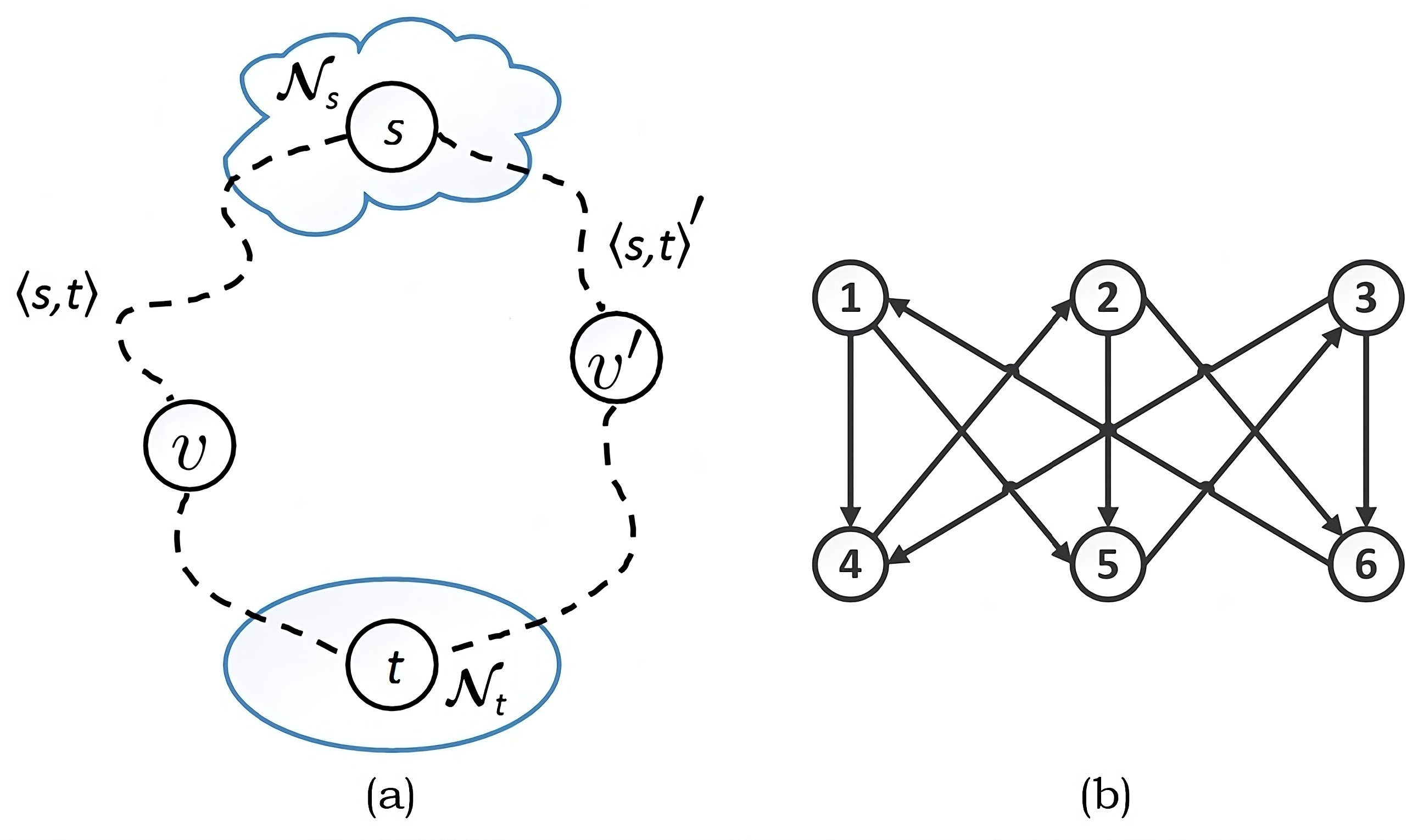
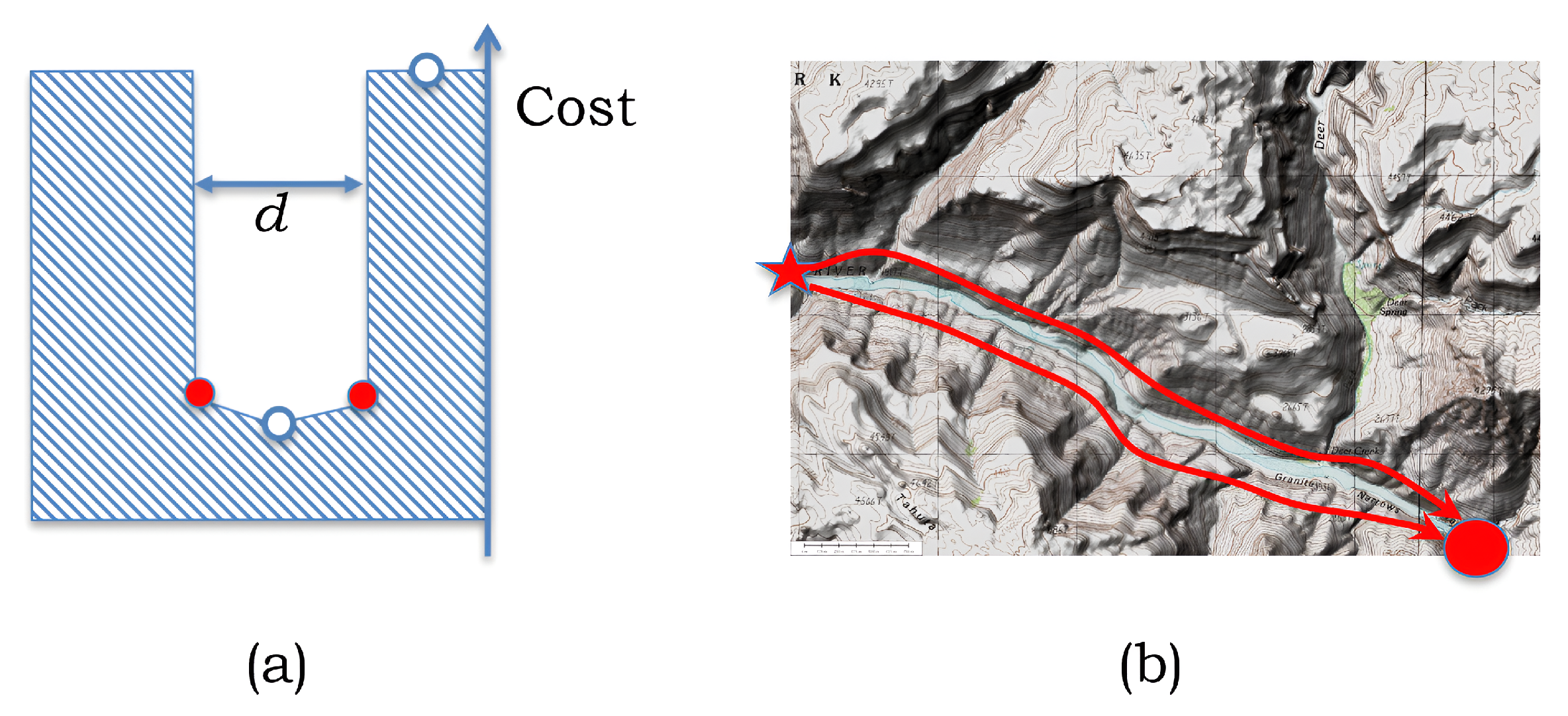
Table 1.
Average run-time in seconds for 3D least-cost path: out-of-the-box vs. layered approach.
| K | 100 | 150 | 200 | 250 | 300 |
|---|---|---|---|---|---|
| Building 3D adjacency matrix | 5.27 | 25.21 | 51.03 | 151.74 | 270.61 |
| Dijkstra’s algorithm | 1.36 | 10.25 | 31.18 | 79.64 | 284.01 |
| Layered approach | 3.05 | 5.85 | 8.86 | 19.55 | 29.23 |
Table 2.
Layered approach run-time in seconds with OpenMP.
| K | 500 | 600 | 700 | 800 | 900 | 1000 |
|---|---|---|---|---|---|---|
| Run-time | 4.85 | 8.22 | 12.87 | 19.12 | 31.80 | 37.84 |
Table 3.
Average run-times in seconds for MIP- and 3D embedding-based approaches.
| K | 5 | 10 | 20 | 50 | 100 | 200 |
|---|---|---|---|---|---|---|
| 0-1 LP relaxation | 0.99 | 1.50 | 5.60 | 43.13 | 422.89 | 4635.73 |
| Building 3D adjacency matrix | 0.0026 | 0.0063 | 0.042 | 0.59 | 5.27 | 51.03 |
| Dijkstra’s algorithm | 0.0007 | 0.0013 | 0.0084 | 0.15 | 1.36 | 31.18 |
Disclaimer/Publisher’s Note: The statements, opinions and data contained in all publications are solely those of the individual author(s) and contributor(s) and not of MDPI and/or the editor(s). MDPI and/or the editor(s) disclaim responsibility for any injury to people or property resulting from any ideas, methods, instructions or products referred to in the content. |
© 2024 by the authors. Licensee MDPI, Basel, Switzerland. This article is an open access article distributed under the terms and conditions of the Creative Commons Attribution (CC BY) license (https://creativecommons.org/licenses/by/4.0/).
Share and Cite
MDPI and ACS Style
Jha, A.; Song, H.; Zinchenko, Y. Resilient Network Design: Disjoint Shortest Path Problem for Power Transmission Application. Systems 2024, 12, 117. https://doi.org/10.3390/systems12040117
AMA Style
Jha A, Song H, Zinchenko Y. Resilient Network Design: Disjoint Shortest Path Problem for Power Transmission Application. Systems. 2024; 12(4):117. https://doi.org/10.3390/systems12040117
Chicago/Turabian StyleJha, Amit, Haotian Song, and Yuriy Zinchenko. 2024. "Resilient Network Design: Disjoint Shortest Path Problem for Power Transmission Application" Systems 12, no. 4: 117. https://doi.org/10.3390/systems12040117
Note that from the first issue of 2016, this journal uses article numbers instead of page numbers. See further details here.