Using Agent-Based Modeling to Assess Liquidity Mismatch in Open-End Bond Funds


1
Muma College of Business, University of South Florida, 4202 East Fowler Avenue, Tampa, FL 33620, USA
2
FinaMetrics LLC, Tampa, FL 33647, USA
*
Author to whom correspondence should be addressed.
†
These authors contributed equally to this work.
Systems 2017, 5(4), 54; https://doi.org/10.3390/systems5040054
Submission received: 1 October 2017
/
Revised: 18 November 2017
/
Accepted: 28 November 2017
/
Published: 6 December 2017
(This article belongs to the Special Issue Pervasive Simulation for Enhanced Decision Making)
Abstract
:In this paper, we introduce a small-scale heterogeneous agent-based model of the US corporate bond market. The model includes a realistic micro-grounded ecology of investors that trade a set of bonds through dealers. Using the model, we simulate market dynamics that emerge from agent behaviors in response to basic exogenous factors (such as interest rate shocks) and the introduction of regulatory policies and constraints. A first experiment focuses on the liquidity transformation provided by mutual funds and investigates the conditions under which redemption-driven bond sales may trigger market instability. We simulate the effects of increasing mutual fund market shares in the presence of market-wide repricing of risk (in the form of a 100 basis point increase in the expected returns). The simulations highlight robust-yet-fragile aspects of the growing liquidity transformation provided by mutual funds, with an inflection point beyond which redemption-driven negative feedback loops trigger market instability.
1. Introduction
The financial crisis of 2008 again highlighted the complex and evolving nature of the financial system and spurred another round of research into the dynamics of financial crises. New regulations aimed to curb risk taking in areas that were at the center of the crisis and limit the potential for contagion to other financial industry segments (with institutions deemed too-big-to-fail being a primary concern). History shows, however, that the financial industry tends to respond to regulation by re-allocating risks across the system. As a result, crises tend to originate in new areas and rarely copy historical patterns.
In the years following the crisis, credit provision to the corporate sector witnessed significant changes. While bank credit contracted, corporate bond markets showed extraordinary growth. Bonds—transferable debt securities—are an important means by which companies fund their business operations and expansion. Well-functioning bond markets—the mechanisms that connect bond issuers with investors and enable trading between investors—are deemed essential for economic activity and growth.
During the bond market expansion, the risks of investing in bonds increased significantly. With yields at historic lows, bonds offer little compensation for interest rate and credit risks while exhibiting high sensitivity of prices to changes in expected returns. Additionally, concerns around the deterioration of liquidity have taken center stage. The challenges are multi-faceted and include the lack of (pre trade) price transparency, reduced investor heterogeneity (increased “herding” behavior) and the decline in dealer intermediation capacity.
In light of its current evolution, the bond market ranks highly on the list of potential risks to financial stability, prompting regulators (and industry participants) to question its resilience under stress [1]. In this paper, we focus on the potential systemic risk caused by the interaction between impaired market liquidity and the increased reliance on liquidity transformation provided by pooled investment vehicles (such as mutual funds) [2]. The two concerns can be summarized as follows:
- Changes in market micro-structure have led to reduced market liquidity and increased liquidity fragility (the tendency of liquidity to evaporate under conditions of stress).
- The growing role of mutual funds in bond markets introduces stability risks from rising liquidity transformation in the presence of redeemable shares. Mutual funds contain redemption features that make them susceptible to runs potentially triggering fire sales and price swings similar to those associated with the activities of participants who rely on short-term debt financing.
Over the last few years, both hypotheses have received ample attention from practitioners, regulators and the academic community without reaching consensus on the scope and severity of the issues. We intend to contribute to the discussion using a somewhat different approach and explore the conditions under which a run on mutual funds can lead to instability. In this paper, we seek to assess the significance of the price feedback loop associated with mutual fund redemption behavior. We use agent-based modeling (ABM) and simulation to better understand the endogenous price dynamics following a market-wide reassessment of risk (using a 100 basis point increase in expected bond yields). We analyze the impact of redemption driven feedback loops under increasing mutual fund participation levels (using market shares of 15%, 25% and 35%).
2. Corporate Bond Market and Liquidity Transformation
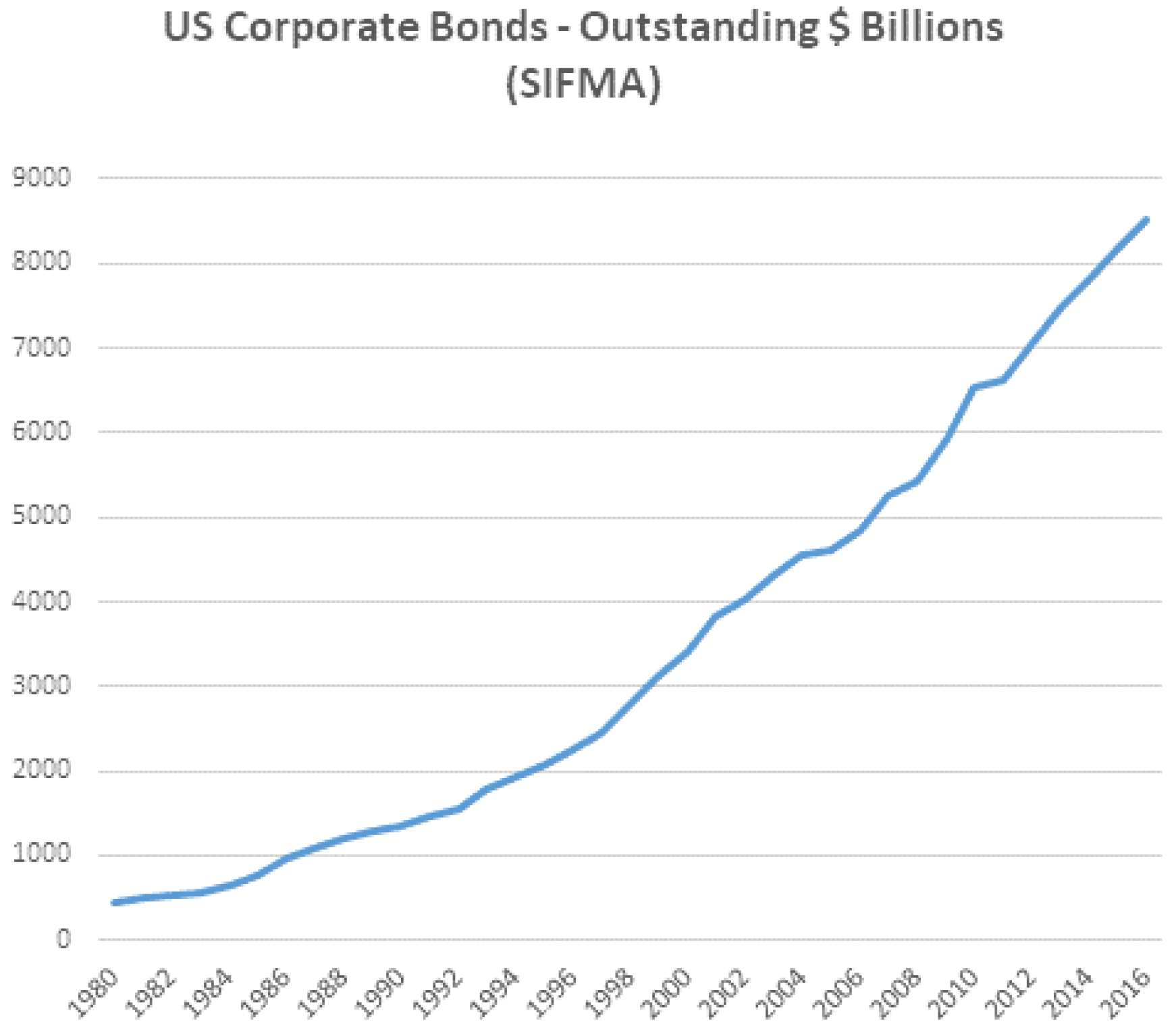
The US corporate bond market has experienced remarkable growth over the past 25 years, with continued expansion following the financial crisis. Analysis of SIFMA (Securities Industry and Financial Markets Association) data points to the overall US corporate bond market expanding from $5.2 trillion in outstanding nominal (Q4 2007) to over $8.5 trillion (Q3 2016) (see Figure 1). Market growth is equally remarkable when measured relative to GDP. Between 2007 and 2015, the investment grade (IG) sector nearly doubled in relative size, with the outstanding nominal relative to GDP increasing from approximately 15% to 30%.
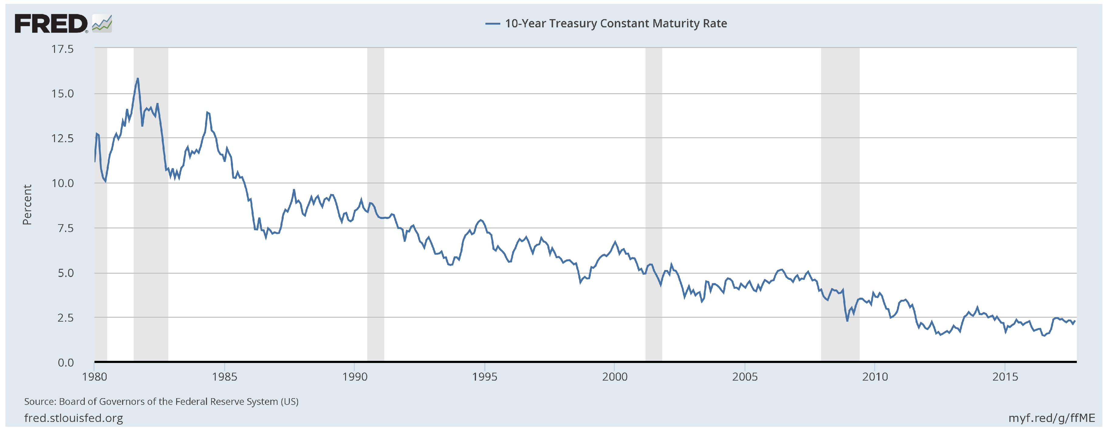
The expansion of the bond market coincided with decreasing risk premiums and increasing price risks. In the current low yield environment, bond prices (which behave inversely to yields) are very sensitive to changes in expected returns, with small increases in interest rates or credit spreads triggering significant drops in bond prices (a feature known as convexity). Figure 2 highlights the remarkable secular decline in the 10-year Treasury yield, often used as a benchmark for evaluating relative yields on corporate bonds.
In addition to convexity, price risk in the overall market has further increased due to a lengthening of the maturity of the outstanding bonds (a longer maturity implies higher price sensitivity) and a decline in overall credit quality. Faced with historically low yields, issuers have been eager to lock in “low rates for longer” through the issuance of bonds with longer maturities (see Figure 3). Overall credit quality has declined as well. Table 1 shows the credit distribution of the IBoxx index (an index of European investment grade corporate bonds). In 2007, BBB rated bonds (the lowest rating in the investment grade category) accounted for 27% of the index; by 2017, the share of BBB bonds in the index increased to 49%. Similar observations apply to the US corporate bond sector, where borrowers with lower credit ratings make up for an increasingly large share of the market. Between 2010 and 2017, the Merrill Lynch US investment grade corporate bond index saw the relative share of bonds with BBB ratings increase from 38% to nearly 48%.
Reflecting on the increased fundamental risk in global bond markets, Jeffrey Gundlach (CEO of Doubleline Capital) was recently quoted in the Financial Times (see below).
“With rates near the lowest levels ever and duration at literally the highest level ever, it is the worst possible set-up versus history. You are [taking] more risk and getting less reward”
Given the combination of increased risks and growing importance of the corporate bond sector, concerns around the proper functioning of its secondary market have taken center stage. Central to the concerns is the deterioration of liquidity, which relates to the ability of market participants to buy or sell a given quantity of bonds, with reasonable immediacy, at low cost, without triggering an outsize impact on price [5]. In a rising rate environment, investors who look to sell bonds will likely face an increasing “illiquidity” discount, further adding to negative price pressure.
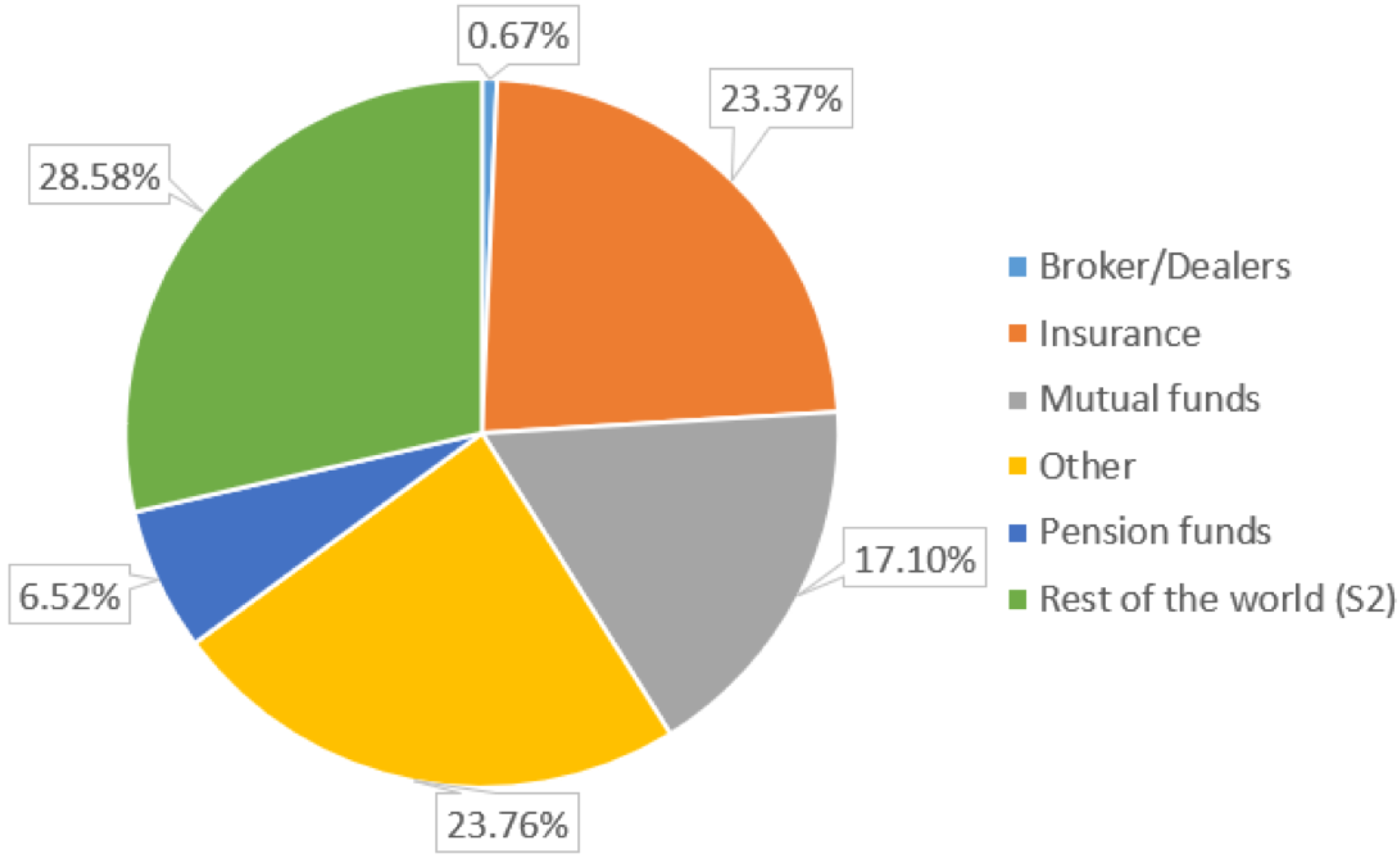
The decline of liquidity is particularly concerning when viewed in the context of the changing corporate bond investor base. Historically, corporate bonds were primarily held by institutional investors with a long investment horizon (such as life insurance companies and pension funds) seeking a steady income stream with limited principal risk. Over the past 20 years, however, the market share of “buy-and-hold” investors has continually decreased in favor of new categories of investors such as mutual funds. Using Federal Reserve data, we estimate that mutual funds accounted for roughly 1.7% of the corporate bond market at the beginning of 1981 (see Figure 4). By the end of Q3 2016 (see Figure 5), the mutual fund market share had increased to around 17% (this excludes holdings of exchange traded funds, which account for an additional 2.8% of the market).
The emergence of mutual funds as significant players in bond markets presents some unique risks. Mutual funds contain redemption features that make them susceptible to withdrawal patterns that resemble classic “run” behaviors potentially triggering fire sales and price swings similar to the activities of participants who rely on short-term (runnable) debt financing. Recent research highlights multiple mechanisms that could lead to disruptive selling by mutual funds, including a first-mover advantage associated with redemption externalities [7] and the dynamic management of cash holdings to buffer against future redemption risk [8]. Empirical studies document return-chasing behavior of mutual fund investors and a significant flow–performance relationship (rising prices trigger fund inflows which contribute to rising prices, the opposite logic applies to falling prices). Funds with illiquid assets exhibit stronger sensitivity of outflows to past performance than funds with liquid assets [7].
When faced with major redemptions, a fund may need to sell its holdings in order to pay out redemptions. Forced selling of bonds in an illiquid market causes further price drops, which, in turn, leads to more investor redemptions. In a downward market, bond funds can therefore introduce a powerful negative feedback loop which—through the various contagion mechanisms—can spill over to other asset markets and impact the real economy [9].
In the simulations described here, we analyze redemption-driven feedback loops following market-wide repricing of risk premiums (using an increase in the required yield). The increase in yield leads to drops in the fundamental value of bonds, with the magnitude of the initial price drops determined by the characteristics of each bond’s cash flow pattern (duration and convexity). However, the feedback loop caused by investor redemptions and forced liquidations is likely to lead to further price decreases and perhaps panic-driven behavior. Our goal is to isolate these effects and eventually study how proposed regulatory policies could improve stability.
3. Agent-Based Modeling and Simulation
Agent-based modeling and simulation have been applied to financial markets in many creative ways, starting with early work on artificial financial markets (such as the Santa Fe artificial stock market) [10]. For an interesting review of influential early projects (see [11]), and, for a more wide ranging (and very entertaining) look at agent-based modeling in finance, see [12]. Of course, simulation methods (apart from agent-based approaches) have been used to study economic phenomena for a long time. For example, Stigler’s pioneering work that uses Monte Carlo simulations to study trading behaviors in securities markets dates back to 1964 [13]. As further noted in [12], Kim and Markowitz developed one of the first “multi-agent” models to investigate the 1987 stock market crash [14]. Their model has two agent types, “rebalancers” and “portfolio insurers” that trade stocks and hold cash balances. Rebalancers simply aim to keep their portfolios evenly split between the two asset classes. Portfolio insurers use a “constant proportion portfolio insurance” (CPPI) method to maintain the portfolio risk level in relation to an insurance expiration date. The simulation results highlight the destabilizing nature of portfolio insurers and provide at least a partial explanation for crisis dynamics like the 1987 crash. The work of Hommes and in ’t Veld provides a much more recent example of modeling booms and busts using heterogeneous agents [15]. In this model, two agent types (fundamentalists and chartists) share knowledge of fundamental prices but take different views on how long price trends last. Fundamentalists hold beliefs around mean-reversion of prices, while chartists look to momentum and the belief that trends tend to continue. The agents can gradually switch beliefs based on performance, which leads to amplifications of booms and busts.
The Office of Financial Research (OFR) has published various papers discussing the value of ABM in the analysis of financial systemic risk (for example, see [16]). Furthermore, the European Commission sponsored a major research initiative (CRISIS, the Complexity Research Initiative for Systemic Instabilities), which aims to analyze systemic risks to the financial sector and the wider economy using ABM. Agent-based approaches have not been applied nearly as widely as DSGE (dynamic stochastic general equilibrium) and econometric models [17]. While most of the existing literature around the application of ABM to finance is focused on equity markets (with some interesting applications to currency and housing markets), we aim to analyze the liquidity conundrum in the corporate bond market (as outlined in Section 2 above).
Our work draws heavily on the strong foundation of prior agent-based models, including advice on how to pursue this type of research [18]. Our focus is squarely on crisis dynamics following some of the prior work cited. However, our work is marked by several important differences:
- Most prior agent-based models focus on central limit order book market structures (as in most equity markets).
- Our corporate bond market model is a decentralized dealer-based quote-driven market, selected since it is considered at risk by many regulatory organizations. Corporate bond markets have been the subject of only one other recent agent-based model [19].
- The agents are drawn from real-world participants based on their investment mandates, constraints and the nature of their liabilities.
- The agent implementations follow empirical (micro-grounded) financial literature, such as the Treynor model of the dealer function [20].
Traditional approaches to micro-prudential risk management, including stress tests and portfolio risk analytics such as Value-at-Risk (VaR), focus on the resilience of individual firms to specific shocks. They fail to address the broader question of how stress might be transmitted among firms through the dynamics of contagion and fire sales. Agent-based modeling and simulation can capture the second order effects of interactions and feedback loops as it models the reaction functions (or behavior) of individual agents. It is particularly well-suited to the analysis of the endogenous nature of liquidity dynamics under stress [21].
Numerous studies have attempted to shed light on the changing liquidity conditions. Opinions differ, however, on the significance of the problem, its root causes and potential fixes. Due to limited data availability (or lack of transparency), most liquidity analyses rely on executed transactions and can only paint a partial picture of liquidity [22]. Furthermore, historical analyses may not adequately capture the dynamics under stress conditions (which is the fundamental concern); liquidity is typically ample during normal (steady-state or equilibrium) market operations but tends to evaporate under conditions of stress. These are the issues we aim to explore using a heterogeneous agent-based model of the corporate bond market.
3.1. Why Agent-Based Modeling?
At this point, it is worth considering why agent-based modeling is a reasonable methodology for investigating economic phenomena. In our view, agent-based approaches are particularly well-suited for modeling financial markets, often complex ecosystems of heterogeneous agents. Economic modeling typically proceeds from theory, through mathematical model formulation, toward better understanding of the economic system being studied. This top-down approach employs abstractions that focus more on representative agents and common behaviors expressed in aggregation. Agent-based modeling uses simulation, based on the interactions of autonomous heterogeneous agents, to generate the emergent behaviors of complex systems (and hopefully inform theory). This more bottom-up approach starts with a characterization of the ecosystem and proceeds through the implementation of heterogeneous agent behaviors (and interactions) towards understanding and theory refinement. The record of more traditional economic models in understanding crisis dynamics is not good. Agent-based models may provide some help in understanding economic systems, especially under conditions of stress. For a persuasive and much more expansive case for agent-based modeling, see Richard Bookstaber’s recent book The End of Theory [21]. Some of the factors that favor agent-based modeling are outlined below:
- Heterogeneous agents: As noted above, agent-based approaches rely on the interactions of heterogeneous agents to generate emergent behaviors of interest. The bond market model described here uses a small (at least to start) set of agent classes to represent a mix of bond investor types with decision-making behaviors anchored in the finance literature.
- Emergent phenomena: Complex system-wide dynamics arise from the interactions between individual agents making simple decisions such as firms trading in a market. Agent-based modeling is based on the actions and interactions between individual autonomous synthetic agents implemented with important behaviors encoded as decision-making algorithms. Basically, the ABM approach is all about emergent system dynamics (simple rules, complex behaviors).
- Non-ergodic processes: Individual actions and interactions that take into account prior context make each simulation pathway potentially unique. As Bookstaber suggests: Does history (and context) matter?—for roulette, no; for human behavior, typically an emphatic yes.
- Radical uncertainty: Emergent phenomena and non-ergodic processes lead to unanticipated uncertainty (“black swans”) or “the things we do not know we do not know” (as noted by D. Rumsfeld, US Secretary of Defense). These unknowns are exactly the type of phenomena that characterize crisis dynamics.
- Computational irreduciblity: Complex systems, based on context-driven interactions, can often be understood only by tracing out the entire path over time (using simulation rather than mathematical shortcuts). This makes agent-based modeling and simulation a natural fit for studying systems like financial markets.
4. An Agent-Based Model of the Corporate Bond Market
The bond market agent-based model implements a somewhat stylized investor ecology, with participants trading a limited universe of bonds through dealers who provide transaction immediacy on a principal basis using a request-for-quote (RFQ) protocol. In selecting the set of agents, we aim to model representative corporate bond investor heterogeneity. While there are multiple ways to segment the investor base, we guided our selection of buy-side agents by the nature of their liabilities (leveraged versus non-leveraged, presence of inflows/outflows) and their investment mandate (passive versus active, long only versus long/short). As as result, the market model includes three buy-side agent classes representative of a mutual fund, an insurance company and a hedge fund.
Out of the three types of buy-side agents, two represent “real money” investors (using no leverage), while the third maintains leveraged positions. Real money investors cannot maintain short positions (must be “long only”); these include an insurance company (typical value investor) and a mutual fund (using passive index tracking). The leveraged investor represents an unconstrained participant (such as a hedge fund) who can maintain both long and short positions.
Recent analysis from the Office of Financial Research (OFR) highlights the importance of financial networks in understanding contagion risk and presents a model of the financial system as a multilayer network (see Figure 6). In line with this multi-layer network view, we modeled interactions between agents using three distinct but interconnected layers representing asset, funding and collateral markets. While our analyses focus on asset price dynamics, there are critical dependencies on the flow of funding (interaction between market liquidity and funding liquidity) and collateral movement. The funding layer focuses on the role of leverage and its impact on fire sales (including feedback loops and cross-asset contagion). It includes critical constraints for leveraged market participants (such as hedge funds and broker-dealers). The collateral layer supports the asset layer (short sales) and funding layer (secured financing) and models the flow of collateral through securities’ lending arrangements and “repo” transactions.
In addition to the three layers of the bond market, the model includes a few direct and indirect linkages with other asset verticals, including equities and government bonds. Equity markets impact the model through the behavior of one of the buy-side agents (an insurance company) that re-balances positions between equities and bonds based on equity market volatility (as well as absolute yield levels). Government bond markets furthermore provide the risk free yield curve, which is used as an input to the bond pricing equation.
In summary, we developed heterogeneous agent classes based on two important dimensions that reflect the real ecology of the US corporate bond market.
- Investment mandate: The investment mandate or policy is perhaps the most important criterion since it encompasses the goals of the organization. Key factors here include the investment horizon and any performance benchmarks (like the Bloomberg Barclays US Aggregate Bond Index). Is the investment vehicle passively or actively managed? Can both long and short positions be held or is it long only? These factors map nicely to the asset layer in the multi-layer network view of the financial system (see Figure 6). Basically, the mandate constrains the decision-making options and as such is central to implementing an agent class.
- Nature of liabilities: The key factor is leverage with respect to the nature of any liabilities. For example, the hedge fund agent class relies heavily on leverage, while the insurance company does not borrow at all. Are the liabilities more or less runnable? Clearly, an open-ended vehicle such as a mutual fund is subject to investor redemptions at any time, creating inflows and outflows based on performance (or anything else that affects the whims of skittish investors).
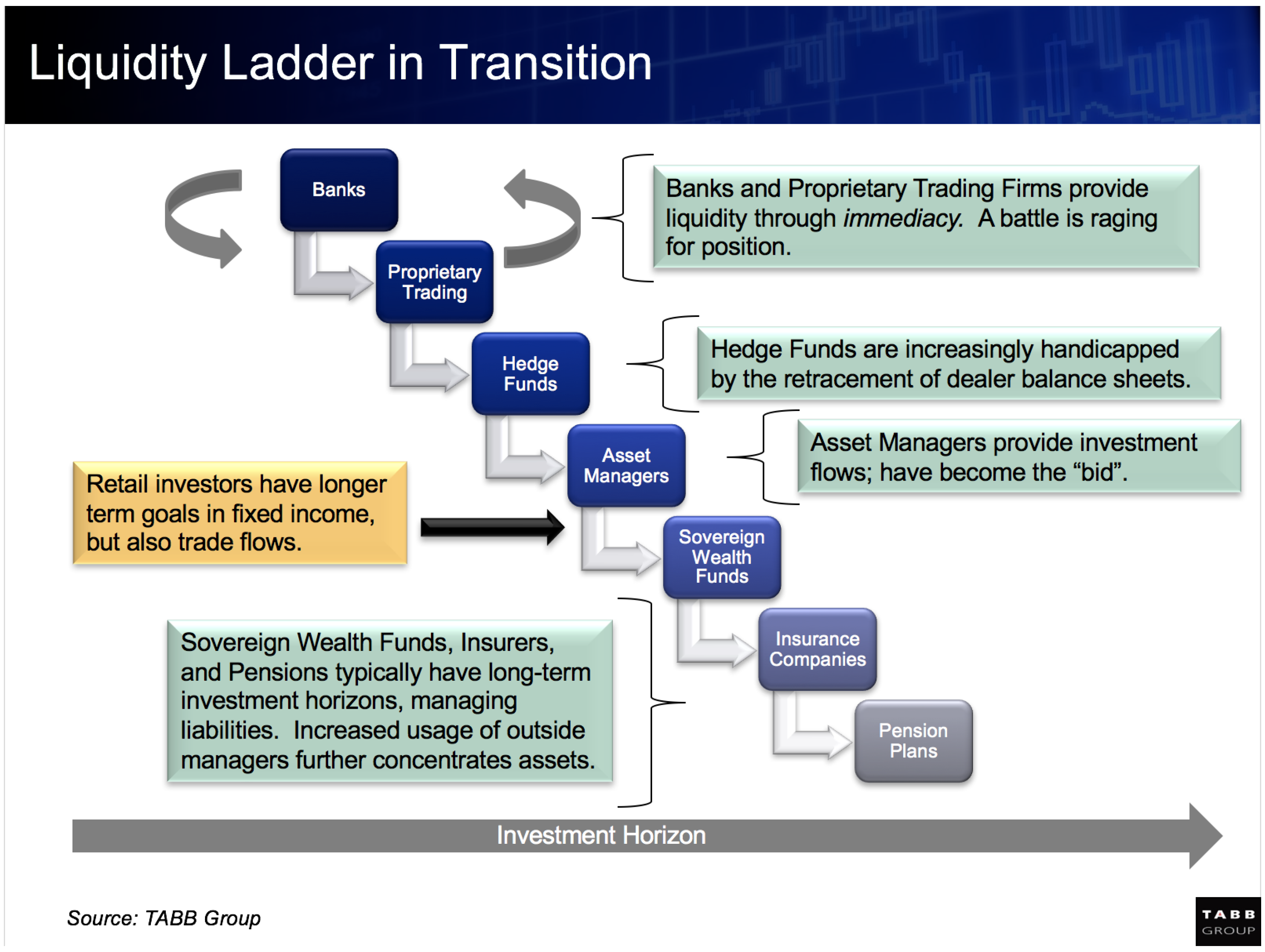
In addition to these two dimensions, other taxonomies of bond market investors informed our choices, including buy-side agents based on mutual funds, insurance companies and hedge funds. The first of these taxonomies is drawn from the Federal Reserve Flow of Funds data referenced in Figure 4 and Figure 5. This data is used to develop the approximate market shares reflecting the real investor ecology. The “liquidity ladder” (from the Tabb Group) is a another reasonable way to organize investor types (see Figure 7 and Table 2). At the top of the ladder, we find our sell-side dealers (mapped to banks and proprietary trading firms). Further down the ladder, we find our hedge funds and mutual funds (mapped to asset managers). We then use insurance companies to capture the investors with longer term investment horizons (including sovereign wealth funds and pension funds). Finally, a more recent paper from the Bank of England used detailed regulatory bond market data to cluster the behaviors of “dealer banks, non-dealer banks, insurance companies, hedge funds, and asset managers” [24]. Again, we find support for our sell-side broker-dealer agents, and buy-side agents based on insurance companies, hedge funds, and mutual funds (as asset managers). The non-dealer banks represent less than 4% of the US corporate bond market, so we left that agent class out for now.
4.1. Mutual Fund Class
The mutual fund acts as a real money investor who aims to replicate the performance of a defined benchmark that includes the full universe of bonds available in the initial model. Any dividends or capital gains distributions are assumed to be re-invested. As noted, the fund is long only and does not leverage positions. The fund also maintains a dynamic cash balance as a buffer against investor redemptions (limiting forced sales) and to minimize transaction costs by parking cash until sizable orders can be made.
4.2. Insurance Company Class
The insurance company agent implements a long-term value investor with a liability driven investment strategy. This agent manages an investment portfolio across equity and fixed income markets and changes allocation between markets depending on overall market conditions. The insurance company is a “long only” investor with additional constraints limiting the concentration of risk in any specific bond. In the initial model, leveraged positions cannot be established (another real money investor) and we further assume there are no external inflows or outflows in the form of premiums or claims.
Trading activity for the insurance company results from changes in portfolio allocation between equity and fixed income markets. Macro allocation decisions are driven by a number of variables, including equity market volatility, as well as the current level and slope of the yield curve. Time series of equity volatility measures such as the VIX are loaded into the model, so different time periods can be used to anchor the simulations in realistic business cycles.
4.3. Hedge Fund Class
The hedge fund agent acts as a short-term tactical trader who follows a relative value trading strategy. As such, the hedge fund maintains both long and short positions and makes active use of leverage. In the real world, fixed income relative value hedge funds have historically been among the most leveraged market participants.
The hedge fund agent is not subject to external inflows (basically a closed end fund) or redemptions (assume investor lock up); its trading capacity is constrained only by the availability of secured financing (leverage) from broker-dealer agents. We assume the hedge fund finances all positions on margin through prime-brokerage style arrangements with some of the dealers. Broker-dealers limit leverage using security-specific haircuts that can be dynamically adjusted depending on market conditions.
All margining is assumed to occur on an overnight basis. At the start of each trading day (a tick in the agent-based simulation), margin requirements are calculated based on current market prices and security-specific haircuts, as set by the broker-dealer agents. The difference between margin requirements and current wealth determines the trading capacity. If the new margin requirements exceed current wealth, the hedge fund is forced to liquidate positions (de-leverage) to meet margin calls. Any excess wealth is free to be invested.
4.4. Broker-Dealers and the RFQ Protocol
Dealers respond to requests for quote (RFQ) from the buy-side agents and trade with clients on a principal basis (there is no inter-dealer market in the initial model). Asset owners must trade with the dealer offering the lowest price. Dealers can maintain both long and short positions. Dealer behavior is limited through regulatory constraints and market discipline, the latter expressed through a constraint on value-at-risk (VaR) relative to capital.
5. Mutual Fund Redemption Experiments: Model Setup
In order to assess the significance of a negative price feedback loop caused by mutual fund redemption behavior, we run agent-based simulations using a simplified model which includes only two agent types: mutual funds and dealers. We model dynamics in the asset layer of the model, without any restrictions in the funding or collateral layers (dealers have unlimited access to financing and there are no restrictions on collateral availability).
5.1. Mutual Funds
Purchases and sales of bonds by mutual funds are driven by inflows (investor fund purchases) and outflows (investor fund redemptions). In line with empirical findings, we model mutual fund flows as a function of historical returns [25]. The flow-performance relationship exhibits a concave shape, which implies that the sensitivity of outflows (to bad performance) is greater than the sensitivity of inflows (to good performance). We specify the daily flow for a given fund at simulation tick t as a percentage of the fund’s prior daily wealth (NAV) as:
where is the daily return lagged by a day (at the end of the prior simulation tick), is the weekly return lagged by a day, is a binary value (indicator) with value 1 if and value 0 if , is a binary value (indicator) with value 1 if and value 0 if .
Using data on corporate bond index returns and fund flows between 1991 through 2014, model parameters were calibrated as follows: , , , , .
Investor inflows and redemptions affect the fund’s cash position, which is managed to a target cash-to-assets ratio of 5% with a lower bound of 3% and an upper bound of 8%. When the cash position exceeds the upper bound, the fund must put cash to work by buying bonds using the index weights. In the opposite direction, the fund must liquidate a portion of the portfolio if redemptions cause the projected end-of-day cash position to drop below the lower bound. The buying and selling behaviors rank the bonds based on current departures from the index and then try to complete trades bond-by-bond until the free cash is invested (or necessary cash is raised). The behaviors are asymmetrical in that buying a specific bond can be postponed until the next tick if no dealer can be found. However, selling is a bit more aggressive in that the agent attempts to raise the necessary cash using any bonds that can be traded.
5.2. Dealers
Dealers are the essential price setters in the initial model. Given the intent to trade, asset owners make a request-for-quote (RFQ) to all dealers. Dealers must respond with “no quote” or a full quote for the requested order size (no partial order fills are allowed for now).
Dealers quote prices using a spread to the bond’s fundamental value (in the initial model, the last traded price reflects fundamental value). Spread calculations are based on inventory positioning considerations and follow the logic outlined by Treynor, using the following assumptions [20].
- Dealers are subject to inventory concentration limits which dictate the maximum long or short position a dealer can hold in a given bond. Inventory limits are set to 10% of outstanding nominal for long positions and 7.5% for short positions.
- Within the inventory limits, dealers quote prices with a view on maximizing client flow.
- We assume the existence of a community of value investors who provide the “outside spread” faced by the dealers. The outside spread sets the price at which dealers can unload a position when it approaches inventory limits. Model values for the outside spread(s) are set as follows: outside bid spread = 100 bps, outside ask spread = 125 bps.
- Dealers specialize in specific bonds based on maturity. Dealer specialization coefficients model the depth of the dealer’s franchise in a given bond as the percentage of the overall value investor community covered by the dealer’s sales force (see Table 3, note the five bonds are named MM101-105). Dealer specialization coefficients are set as follows.
- -
- An inventory spread is calculated using a step function, with the maximum spread equal to the outside spread applicable to the dealer.
- -
- The inventory spread is adjusted slightly (increased in case of a bid, lowered in case of an offer) if the dealer can cover any part of the request out of inventory; that is: the inventory spread is increased on a bid quoted against a short position and lowered on an ask quoted against a long position. The amount of the inventory spread adjustment is dependent on dealer specialization and is proportional to the fraction of the quote that can be serviced out of inventory.
- The quoted price in response to an RFQ is equal to the last traded price adjusted for the spread as calculated above.
5.3. Market Universe and T-Zero Starting Conditions
The market universe consists of five tradable bonds (see Table 4 for details). The bonds are identical with respect to structure, form and major covenants including issuer, redemption (bullet redemption at maturity without optionality clauses) and rate provisions (fixed coupon). The bonds differ along only three dimensions:
- Outstanding nominal amount ranges from 500 M to 2 B.
- Maturities cover major points on the yield curve (1, 2, 5, 10 and 25 years).
- Coupon rates range from 1.75% to 4.00%.
At any point in time, all asset owners perceive the same fundamental value for a specific bond. That is, all asset owners use the same valuation model and observe the same input prices. The value for the above five bonds is fully reflected in five data points (a par yield curve with five rates) and a simple calculation of a bond’s price given its par yield.
The starting conditions for the agent-based simulation include:
- Bond index composition with weights based on nominal amount (Table 4, Index Weights).
- Initial par yield curve and bond prices (Table 4, Yield and Price).
- Starting bond holdings are allocated to two buy-side agents: mutual fund and insurance agent. The mutual fund holds either 15%, 25% or 35% of the outstanding nominal in the market, with the remaining nominal held by the insurance agent. The mutual fund is invested across all bonds in the index based on the index weights. All dealers start with square (zero) inventory positions.
In addition, initial endowments for the buy-side agents include:
- Mutual fund: In addition to its bond holdings, the fund has an opening cash position reflecting a 5% cash-to-assets ratio.
- Insurance company: Initial portfolio allocation includes a 60/40 split between fixed income and equity markets (assumed to be invested in a broad market index like the S&P 500).
6. Mutual Fund Redemption Experiments: Model Results
Using the model setup outlined above, we simulate the effect of a 100 basis point rise in expected yields under various mutual fund market shares (using three realistic values: 15%, 25%, and 35%). The magnitude of the chosen shock (100 basis points) is aligned with market risk measures commonly used by regulators and industry participants. In the latest edition of the Global Financial Stability Report, the IMF (International Monetary Fund) estimates losses to fixed income mutual funds following a 100 basis point shock to interest rates [26]. The IMF analysis puts mutual fund losses around 7% of NAV. In our simulations, the 100 basis point shock triggers instantaneous losses in line with IMF calculations (see further discussion in Section 6.1), with fund losses at tick 50 in the simulation reported as 7.2% of NAV. In a research note focused on the first mover advantage in high-yield bond mutual funds, Barclays analysts investigate a variety of market shocks, with the most adverse case amounting to a 10% market drop, about 3% higher than the market correction used in our simulation.
In all experiments, the interest rate shock causes a drop in bond prices and hurts fund returns, thereby causing investors to withdraw funds. At a certain point, a mutual fund needs to liquidate part of the bond portfolio to meet redemptions. These forced sales will cause bond prices to decline further, sparking another round of price drops and redemptions. This type of feedback loop is exactly what we are trying to capture using agent-based modeling approaches.
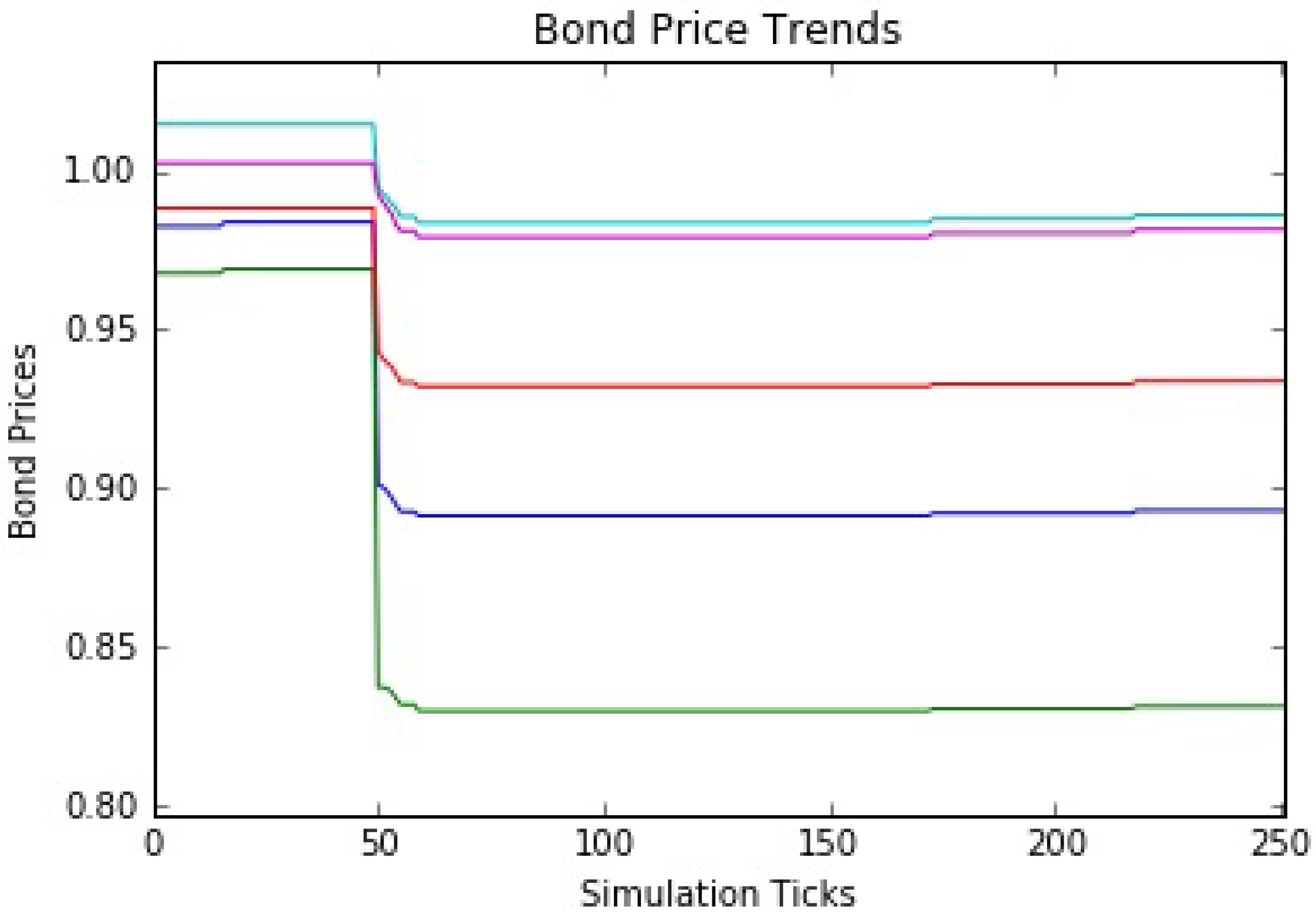
6.1. Mutual Fund at 15% Market Share
The first simulations use a market share of 15%, slightly below the real market share, but a reasonable starting point. The simulations are run for 252 ticks, mirroring the typical number of trading days in a year. An economic shock is delivered at tick 50 in the form of a 100 basis point rise in the interest rate. The corresponding price drops across all five bonds are easily seen in Figure 8. Price changes at tick 50 are due only to the interest rate change and are computed for each bond based on its duration and convexity. Bond prices adjust between 1% to 14% with longer maturity bonds showing higher price sensitivity. At the end of tick 50, re-pricing of the mutual fund bond holdings triggers losses around 7.2% of NAV, in line with IMF analysis (see above).
Following market wide repricing at tick 50, a redemption-driven negative price feedback loop drives more gradual secondary price decreases (in the low 1% range) for the next 10 ticks or so. After the market stabilizes, more normal trading activity returns (in the form of sporadic price increases as investor inflows add funds). Quantitative results are presented for both pre-shock and post-shock prices (see Table 5), as well as for prices at the bottom of the market (see Table 6).
The dynamics of the redemption-driven feedback loop and recovery are outlined in Table 7, which includes weekly investor redemptions for four consecutive trading weeks following the market shock (each week consisting of five ticks). During week 1, investor redemptions equal roughly $172 million, which equates to 23% of the NAV at the start of the week. The fund engages in significant bond sales in order to pay out redemptions, thereby causing bond prices to decline further while yields increase. At the end of week 1, the yield on the bond index has increased by about 120 basis points relative to its value just prior to the market shock. Given the 23% decrease in fund NAV, the yield sensitivity to outflows—measured as the yield increase (in basis points) corresponding to fund redemptions at 1% of NAV—is 5.24 basis points. This measure is aligned with the empirical findings reported in a May 2015 research note from Deutsche Bank in which the authors examine the top 10% largest weekly outflows from high yield (HY) and investment grade (IG) mutual funds along with the coincident spread change during those weeks, and using a trailing-10-episodes-average spread change per percentage fund outflow [27]. During the period between 2004 and 2014, the authors find the spread/flow sensitivity for IG bonds to vary between 2 bps and 30 bps, with the average value prior to the 2008 crisis hovering around 5 bps. This value is aligned with the yield-to-flow sensitivity during our simulation, as reported in the redemption-driven feedback loops during week 1 (5.24 bps) and week 2 (5.13 bps) following the market shock.
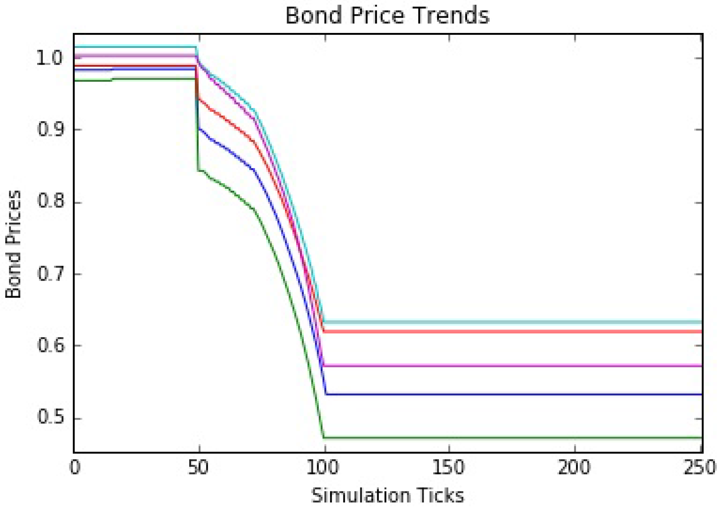
6.2. Mutual Fund at 25% Market Share
The next simulations use a market share of 25%, a reasonable level somewhat above the current situation. Again, the simulations are run for 252 ticks and a 100 basis point interest rate shock is delivered at tick 50. The interest rate hike causes the expected price drops across all five bonds as before (see Figure 9). These shock-induced drops are followed by further drops in prices for the next 10 to 20 ticks due to the redemption-driven feedback loop. As above, the rate hike impacts increase with maturity, showing price drops in the 1% to 14% range. The larger mutual fund market share increases the effects of the feedback loop, with secondary price decreases now in the 1.7% to 2.7% range (see Table 8). This is a definite increase over the first simulation, but the feedback loop still has much less of an effect as compared to the interest rate shock. Once the market stabilizes and normal trading activity returns, there is a somewhat better recovery in prices.
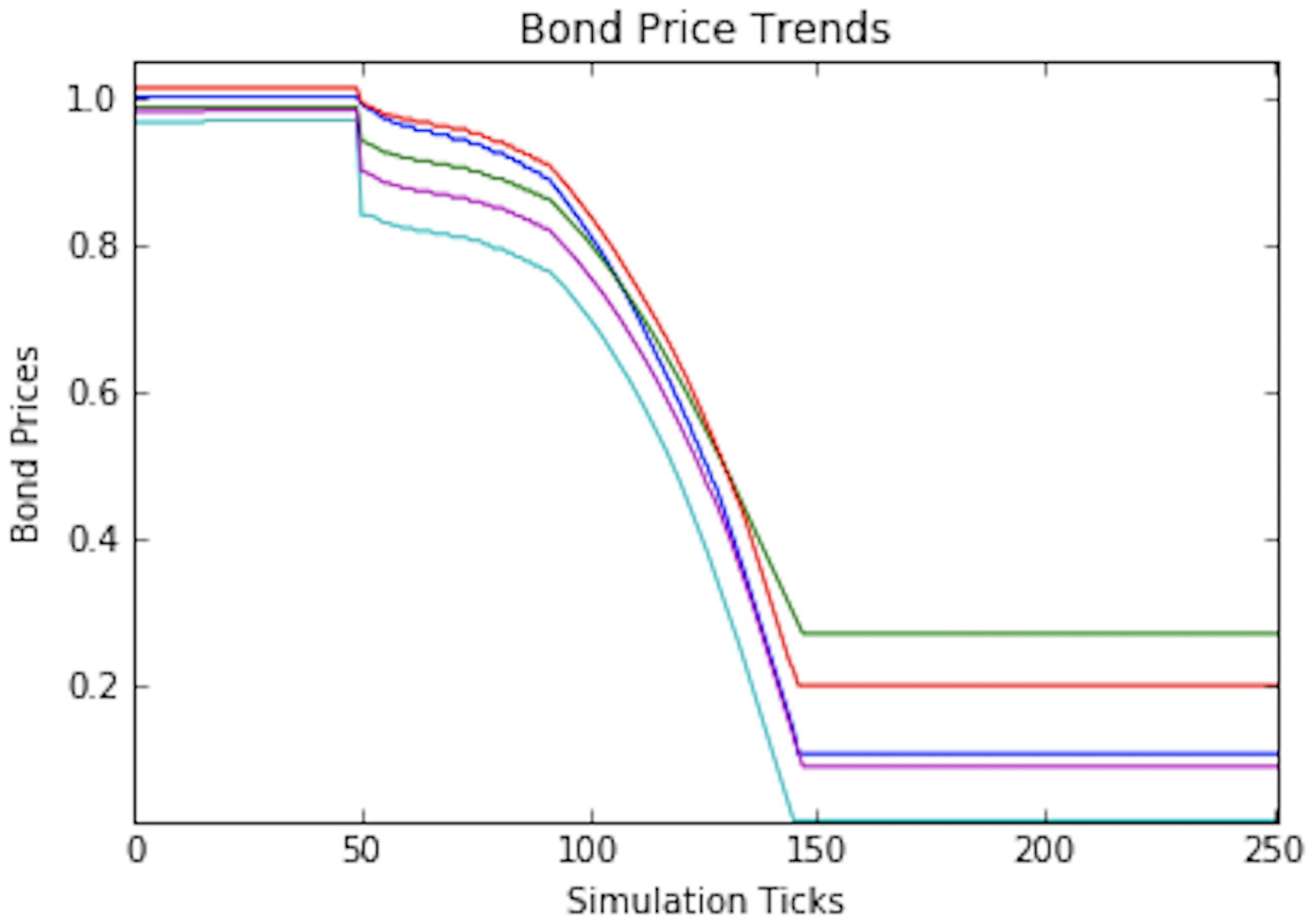
6.3. Mutual Fund at 35% Market Share
The final simulations use a market share of 35%, a substantial increase over the current situation. Again, the simulations are run for 252 ticks and a 100 basis point interest rate shock is delivered at tick 50. The interest rate hike causes the expected price drops across all five bonds as before (see Table 5). However, after that, the simulations take a different path. After these shock-induced drops, the prices fall of a cliff. For the next 50 clicks, the redemption-driven feedback loop causes a spiral of decreasing prices (see Figure 10). In fact, the concave curve means that the price drops accelerate with correspondingly dramatic wealth destruction. The price drops are more pronounced from the outset, but reach an inflection point followed by precipitous price drops until all the dealer capacity is consumed (and the market flatlines). In these simulations, the redemption-driven price drops dwarf the initial interest rate shock effects. The feedback loop causes price drops in the 35% to 44% range, as compared to the shock-induced drops of roughly 1% to 14% (see Table 9).
In actuality, the instability and all out market crashes start to occur at approximately a 30% mutual fund market share (see Figure 11). However, notice that the feedback look is not as severe and overall it takes roughly 50 more trading days (or ticks) to completely crash. We should not read too much into this exact market share level since we aim to use our model to evaluate regulatory policies or re-create market behaviors, not predict specific thresholds. We are much more interested in the emergent behaviors and relative comparisons that can provide useful guidance.
7. Conclusions
In this paper, we introduce an agent-based model of the corporate bond market and obtain realistic market dynamics with a small-scale heterogeneous model. The model includes three buy-side agent classes that provide a nice breadth of different investment approaches. The sell-side agents are broker-dealers who serve as the price setters in the model. This simple model is being used to refine agent behaviors and assess responses to basic exogenous factors and the introduction of regulatory policies and constraints. Our first experiments focus on redemption-driven price feedback loops under increasing fund market shares. The focus is on the mutual fund class in the experiments described here, with economic shocks delivered as the mutual fund market share is increased. As the market share grows, the simulation exhibits realistic feedback loops. First, the prices drop in direct response to an interest rate shock, with secondary redemption-driven feedback loops causing further declines in price, followed by gradual stabilization and recovery. However, at a 35% market share, the model becomes unstable, with the initial shock-induced price drops followed by an accelerating feedback loop that overwhelms the sell-side broker dealers and freezes the market. This is exactly the behavior that concerns both regulators and practitioners. We believe that this agent-based model provides an excellent tool for the evaluation of possible regulatory mechanisms and policies to help minimize future crises.
Acknowledgments
We gratefully acknowledge the support of the National Science Foundation (NSF Award 1445403) and the Office of Financial Research (OFR) in providing funding for this research. For more details, please see the project website at http://GSRisk.org (and Donald J. Berndt’s research page at http://dberndt.link/home).
Author Contributions
Donald J. Berndt and David Boogers conceived and designed the experiments. All authors participated in implementing the agent-based models, performing the experiments and analyzing the data. All authors also contributed to writing and revising the paper.
Conflicts of Interest
The authors declare no conflict of interest. The funding sponsors had no role in the design of the study; in the collection, analyses, or interpretation of data; in the writing of the manuscript, and in the decision to publish the results.
Abbreviations
The following abbreviations are used in this manuscript:
| ABM | Agent-Based Models |
| DSGE | Dynamic Stochastic General Equilibrium Models |
| FINRA | Financial Industry Regulatory Authority (https://www.finra.org/) |
| FRED | Federal Reserve Economic Data (https://fred.stlouisfed.org/) |
| IMF | International Monetary Fund |
| NAV | Net Asset Value |
| OFR | Office of Financial Research (https://www.financialresearch.gov/) |
| RFQ | Request-for-Quote Protocol |
| SIFMA | Securities Industry and Financial Markets Association (https://www.sifma.org/) |
References
- Flood, M.D.; Liechty, J.C.; Piontek, T. Systemwide Commonalities in Market Liquidity; Technical Report, 15-11; Office of Financial Research: Washington, DC, USA, 2015. [Google Scholar]
- Barclays. Mutual Funds and Credit Liquidity, Nobody Move; Barclays Credit Research: New York, NY, USA, 2015. [Google Scholar]
- Board of Governors of the Federal Reserve System (US). 10-Year Treasury Constant Maturity Rate [DGS10]; FRED, Federal Reserve Bank of St. Louis, St. Louis, MO, USA. 2017. Available online: https://fred.stlouisfed.org/series/DGS10 (accessed on 1 October 2017).
- Citi Research. Partying Like It’s 2007; European Credit Weekly: London, UK, 2017. [Google Scholar]
- Roubini, N. The Liquidity Time Bomb. 2015. Available online: https://www.project-syndicate.org/commentary/liquidity-market-volatility-flash-crash-by-nouriel-roubini-2015-05 (accessed on 11 March 2017).
- Board of Governors of the Federal Reserve System (US). Financial Accounts of the United States (Flow of Funds); Federal Reserve System, Washington, DC, USA. 2017. Available online: https://www.federalreserve.gov/releases/z1/current/ (accessed on 1 October 2017).
- Chen, Q.; Goldstein, I.; Jiang, W. Payoff Complementarities and Financial Fragility: Evidence from Mutual Fund Outflows. J. Financ. Econ. 2010, 97, 239–262. [Google Scholar] [CrossRef]
- Morris, S.; Shim, I.; Shin, H.S. Redemption Risk and Cash Hoarding by Asset Managers; Technical Report, 608; Bank for International Settlements: Basel, Switzerland, 2017. [Google Scholar]
- ECB. Shadow Banking in the Euro Area: Risks and Vulnerabilities in the Investment Fund Sector; ECB Occasional Paper 174; ECB: Frankfurt, Germany, 2016. [Google Scholar]
- LeBaron, B.; Arthur, W.B.; Palmer, R. Time Series Properties of an Artificial Stock Market. J. Econ. Dyn. Control 1999, 23, 1487–1516. [Google Scholar] [CrossRef]
- LeBaron, B. Agent-Based Computational Finance: Suggested Readings and Early Research. J. Econ. Dyn. Control 2000, 24, 679–702. [Google Scholar] [CrossRef]
- Samanidou, E.; Zschischang, E.; Stauffer, D.; Lux, T. Agent-Based Models of Financial Markets. Rep. Prog. Phys. 2007, 70, 409–450. [Google Scholar] [CrossRef]
- Stigler, G.J. Public Regulation of the Securities Market. J. Bus. 1964, 37, 117–142. [Google Scholar] [CrossRef]
- Kim, G.W.; Markowitz, H.M. Investment Rules, Margin and Market Volatility. J. Portf. Manag. 1989, 16, 45–52. [Google Scholar] [CrossRef]
- Hommes, C.; in ’t Veld, D. Booms, Busts and Behavioural Heterogeneity in Stock Prices. J. Econ. Dyn. Control 2017, 80, 101–124. [Google Scholar] [CrossRef]
- Bookstaber, R. Using Agent-Based Models for Analyzing Threats to Financial Stability; Technical Report, 0003; Office of Financial Research: Washington, DC, USA, 2012. [Google Scholar]
- Farmer, J.D.; Foley, D. The Economy Needs Agent-Based Modelling. Nature 2009, 460, 685–686. [Google Scholar] [CrossRef] [PubMed]
- LeBaron, B. A Builder’s Guide to Agent-Based Financial Markets. Quant. Financ. 2001, 1, 254–261. [Google Scholar] [CrossRef]
- Braun-Munzinger, K.; Liu, Z.; Turrell, A. An Agent-Based Model of Dyanmics in Corporate Bond Trading; Technical Report, 592; Bank of England: London, UK, 2016. [Google Scholar]
- Treynor, J.L. The Economics of the Dealer Function. Financ. Anal. J. 1987, 62, 27–34. [Google Scholar] [CrossRef]
- Bookstaber, R. The End of Theory; Princeton University Press: Princeton, NJ, USA, 2017. [Google Scholar]
- Edwards, A.K.; Harris, L.; Piwowar, M.S. Corporate Bond Market Transaction Costs and Transparency. J. Financ. 2007, 62, 1421–1451. [Google Scholar] [CrossRef]
- Bookstaber, R.; Kenett, D.Y. Looking Deeper, Seeing More: A Multilayer Map of the Financial System; Technical Report, 16-06; Office of Financial Research: Washington, DC, USA, 2016. [Google Scholar]
- Czech, R.; Roberts-Sklar, M. Investor Behaviour and Reaching for Yield: Evidence from the Sterling Corporate Bond Market; Technical Report, 685; Bank of England: London, UK, 2017. [Google Scholar]
- Goldstein, I.; Jiang, H.; Ng, D.T. Investor Flows and Fragility in Corporate Bond Funds. Technical Report. 2015. Available online: https://ssrn.com/abstract=2596948 (accessed on 1 October 2017).
- IMF. Global Financial Stability Report. 2016. Available online: https://www.imf.org/en/Publications/GFSR/Issues/2017/09/27/global-financial-stability-report-october-2017 (accessed on 1 October 2017).
- Deutsche Bank. US Credit Strategy, Signs of Liquidity Vacuum in Unexpected Places; Deutsche Bank Markets Research: New York, NY, USA, 2015. [Google Scholar]
Figure 1.
US corporate bond market size. Source: SIFMA, data analysis by authors.

Figure 2.
The 30-year decline in 10-year Treasury yields. Source: Federal Reserve Economic Data (FRED) [3].
Figure 2.
The 30-year decline in 10-year Treasury yields. Source: Federal Reserve Economic Data (FRED) [3].

Figure 3.
Average maturity of US corporate bonds (number of years). Source: Financial Times; SIFMA data.
Figure 3.
Average maturity of US corporate bonds (number of years). Source: Financial Times; SIFMA data.
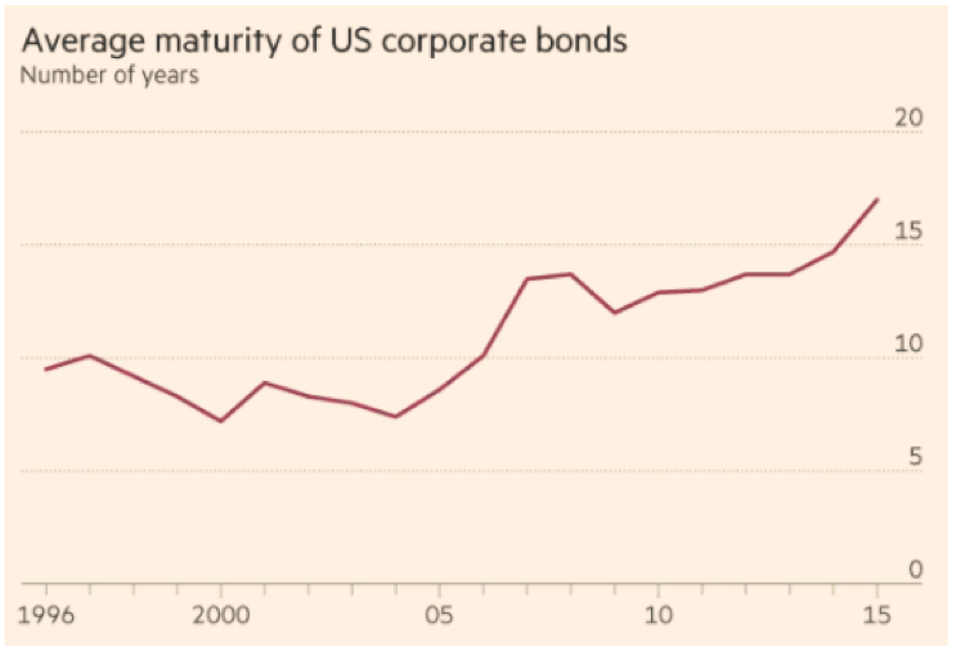
Figure 4.
Investor ecosystem circa 1981 (Q1) by approximate market share. Source: Federal Reserve Flow of Funds data [6], analysis by authors.
Figure 4.
Investor ecosystem circa 1981 (Q1) by approximate market share. Source: Federal Reserve Flow of Funds data [6], analysis by authors.
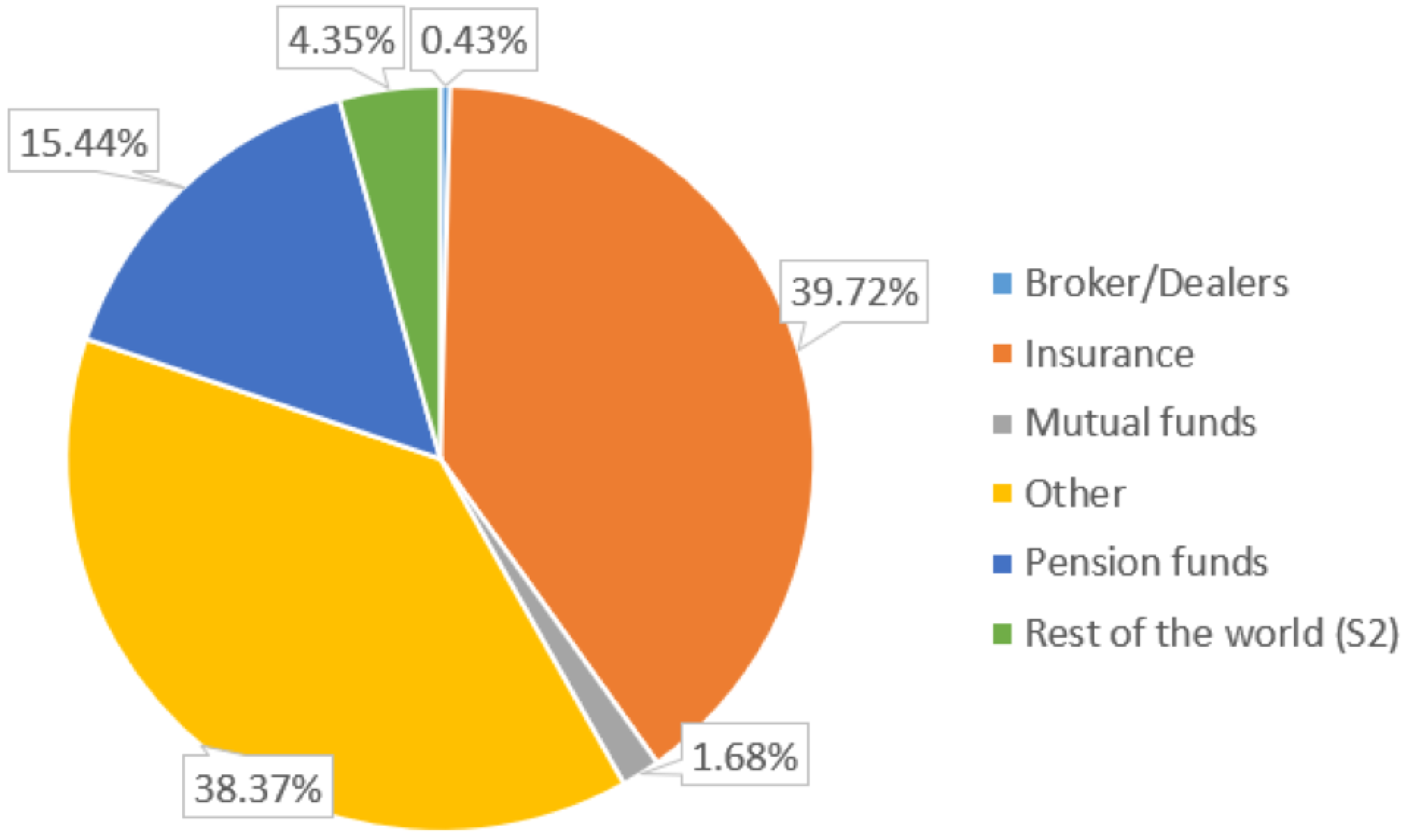
Figure 5.
Investor ecosystem circa 2016 (Q3) by approximate market share. Source: Federal Reserve Flow of Funds data [6], analysis by authors.
Figure 5.
Investor ecosystem circa 2016 (Q3) by approximate market share. Source: Federal Reserve Flow of Funds data [6], analysis by authors.

Figure 6.
The financial system as a multilayer network. Source: Office of Financial Research [23].
Figure 6.
The financial system as a multilayer network. Source: Office of Financial Research [23].
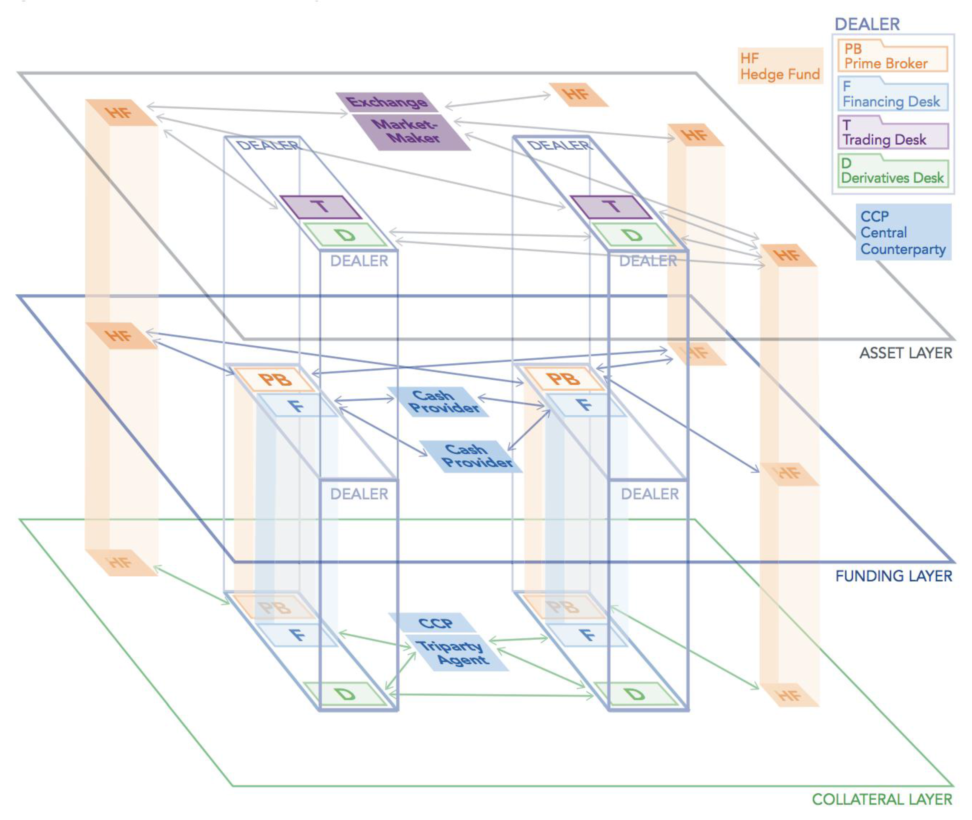
Figure 7.
The liquidity ladder. Source: Tabb Group.

Figure 8.
Bond price trends for a 15% mutual fund market share.

Figure 9.
Bond price trends for a 25% mutual fund market share.
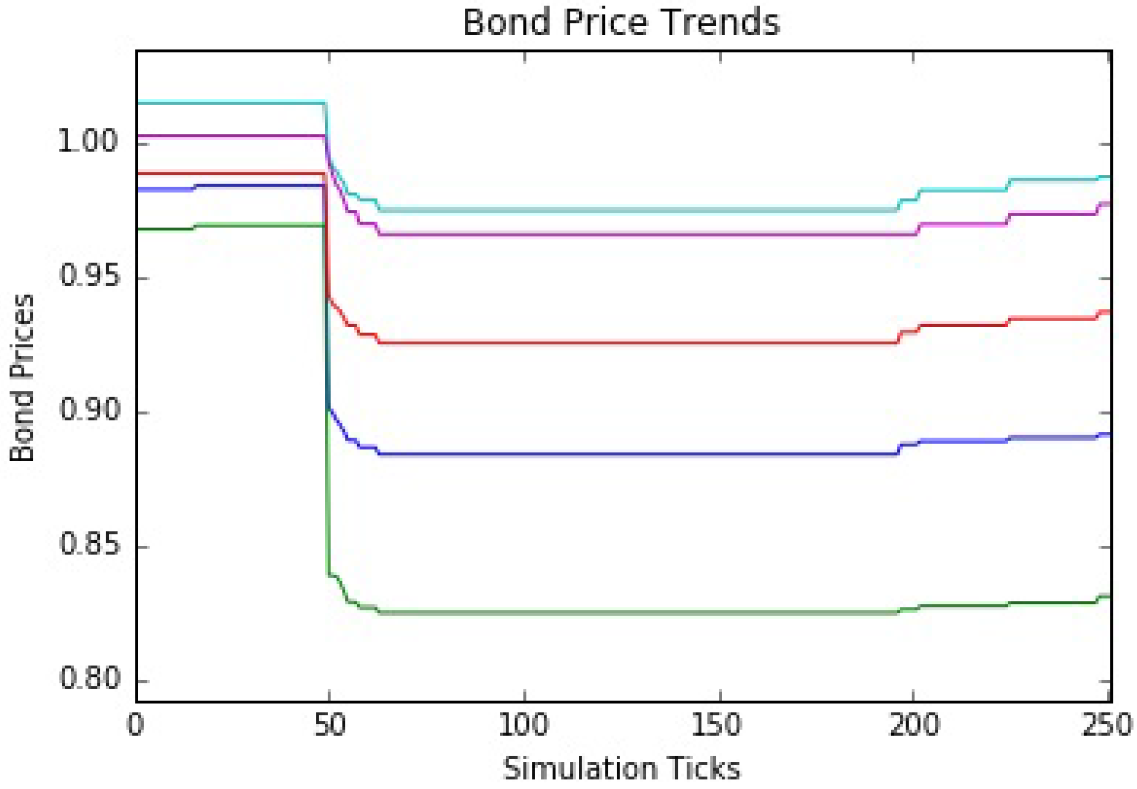
Figure 10.
Bond price trends for a 35% mutual fund market share.

Figure 11.
Bond price trends for a 30% mutual fund market share.


Table 1.
IBoxx index credit rating distribution. Source: Citi Research [4].
Table 1.
IBoxx index credit rating distribution. Source: Citi Research [4].
| Rating | Notional (Euro bn): 2007 | 2017 | Index (%): 2007 | 2017 |
|---|---|---|---|---|
| AAA | 18 | 10 | 3% | 1% |
| AA | 197 | 190 | 27% | 11% |
| A | 319 | 683 | 39% | 40% |
| BBB | 197 | 839 | 27% | 49% |
Table 2.
The liquidity ladder (adapted from the Tabb Group).
| Agent Class | Liquidity Level | Description |
|---|---|---|
| Hedge Funds | High Liquidity | Short-term opportunistic trading with leverage. |
| Mutual Funds | Medium Liquidity | Mixed investments driven by fund inflows/outflows. |
| Insurance Companies | Low Liquidity | Long-term horizon matched to liabilities. |
Table 3.
Dealer specialization across bond maturities.
| Dealers/Bonds: | MM101 | MM102 | MM103 | MM104 | MM105 |
|---|---|---|---|---|---|
| Dealer 1 | 90% | 90% | 75% | 50% | 50% |
| Dealer 2 | 50% | 75% | 90% | 75% | 50% |
| Dealer 3 | 50% | 50% | 75% | 90% | 90% |
Table 4.
Characteristics of tradable bonds.
| Bonds | MM101 | MM102 | MM103 | MM104 | MM105 |
|---|---|---|---|---|---|
| Nominal | 500M | 500M | 1B | 2B | 1B |
| Maturity | 1 Year | 2 Year | 5 Year | 10 Year | 25 Year |
| Coupon | 1.75% | 2.50% | 2.25% | 2.40% | 4.00% |
| Yield | 1.50% | 1.75% | 2.50% | 2.60% | 4.21% |
| Price | 100.247 | 101.468 | 98.832 | 98.249 | 96.772 |
| Index Weight | 10% | 10% | 20% | 40% | 20% |
Table 5.
Initial bond price drops after 100 basis point shock.
| Time (Tick) | Bond | Price | Price Drop (%) |
|---|---|---|---|
| Pre-Shock (49) | MM101 | 100.247 | NA |
| Pre-Shock (49) | MM102 | 101.468 | NA |
| Pre-Shock (49) | MM103 | 98.832 | NA |
| Pre-Shock (49) | MM104 | 98.388 | NA |
| Pre-Shock (49) | MM105 | 96.911 | NA |
| Post-Shock (50) | MM101 | 99.264 | 0.98% |
| Post-Shock (50) | MM102 | 99.517 | 1.92% |
| Post-Shock (50) | MM103 | 94.312 | 4.57% |
| Post-Shock (50) | MM104 | 90.123 | 8.40% |
| Post-Shock (50) | MM105 | 83.725 | 13.61% |
Table 6.
Redemption-driven bond price drops at a 15% mutual fund market share.
| Time (Tick) | Bond | Price | Price Drop (%) |
|---|---|---|---|
| Bottom | MM101 | 97.90 | 1.37% |
| Bottom | MM102 | 98.362 | 1.16% |
| Bottom | MM103 | 93.202 | 1.18% |
| Bottom | MM104 | 89.128 | 1.10% |
| Bottom | MM105 | 82.982 | 0.89% |
Table 7.
Yield reaction to outflows, measured in bps/percentage flow.
| Elapsed Time (Week Since Shock) | Investor Flows (Dollars) | Investor Flows (% NAV) | Index Yield Change (bps) | Yield Reaction to Flows (bps per Percentage Flow) |
|---|---|---|---|---|
| Week 1 | −$171,937,047 | −22.9% | 120 bps | 5.24 bps |
| Week 2 | −$12,263,176 | −2.1% | 11 bps | 5.13 bps |
| Week 3 | −$2,232,899 | −0.4% | 0 bps | 0 bps |
| Week 4 | −$475,590 | −0.1% | 0 bps | 0 bps |
Table 8.
Redemption-driven bond price drops at a 25% mutual fund market share.
| Time (Tick) | Bond | Price | Price Drop (%) |
|---|---|---|---|
| Bottom | MM101 | 96.576 | 2.71% |
| Bottom | MM102 | 97.473 | 2.05% |
| Bottom | MM103 | 92.513 | 1.91% |
| Bottom | MM104 | 88.371 | 1.94% |
| Bottom | MM105 | 82.469 | 1.66% |
Table 9.
Redemption-driven bond price drops at a 35% mutual fund market share.
| Time (Tick) | Bond | Price | Price Drop (%) |
|---|---|---|---|
| Bottom | MM101 | 57.129 | 42.45% |
| Bottom | MM102 | 63.206 | 36.49% |
| Bottom | MM103 | 61.889 | 34.38% |
| Bottom | MM104 | 53.172 | 41.00% |
| Bottom | MM105 | 47.097 | 44.10% |
© 2017 by the authors. Licensee MDPI, Basel, Switzerland. This article is an open access article distributed under the terms and conditions of the Creative Commons Attribution (CC BY) license (http://creativecommons.org/licenses/by/4.0/).
Share and Cite
MDPI and ACS Style
Berndt, D.J.; Boogers, D.; Chakraborty, S.; McCart, J. Using Agent-Based Modeling to Assess Liquidity Mismatch in Open-End Bond Funds. Systems 2017, 5, 54. https://doi.org/10.3390/systems5040054
AMA Style
Berndt DJ, Boogers D, Chakraborty S, McCart J. Using Agent-Based Modeling to Assess Liquidity Mismatch in Open-End Bond Funds. Systems. 2017; 5(4):54. https://doi.org/10.3390/systems5040054
Chicago/Turabian StyleBerndt, Donald J., David Boogers, Saurav Chakraborty, and James McCart. 2017. "Using Agent-Based Modeling to Assess Liquidity Mismatch in Open-End Bond Funds" Systems 5, no. 4: 54. https://doi.org/10.3390/systems5040054
Note that from the first issue of 2016, this journal uses article numbers instead of page numbers. See further details here.