Article

Energy-Efficient FPGA-Based Parallel Quasi-Stochastic Computing

Department of Computer Engineering, Missouri University of Science & Technology, 141 Emerson Electric Co. Hall, 301 W. 16th St, Rolla, MO, 65409-0040, USA
*
Author to whom correspondence should be addressed.
J. Low Power Electron. Appl. 2017, 7(4), 29; https://doi.org/10.3390/jlpea7040029
Submission received: 6 September 2017 / Revised: 26 October 2017 / Accepted: 13 November 2017 / Published: 17 November 2017
(This article belongs to the Special Issue FPGA and Reconfigurable Computing)

Abstract

:
The high performance of FPGA (Field Programmable Gate Array) in image processing applications is justified by its flexible reconfigurability, its inherent parallel nature and the availability of a large amount of internal memories. Lately, the Stochastic Computing (SC) paradigm has been found to be significantly advantageous in certain application domains including image processing because of its lower hardware complexity and power consumption. However, its viability is deemed to be limited due to its serial bitstream processing and excessive run-time requirement for convergence. To address these issues, a novel approach is proposed in this work where an energy-efficient implementation of SC is accomplished by introducing fast-converging Quasi-Stochastic Number Generators (QSNGs) and parallel stochastic bitstream processing, which are well suited to leverage FPGA’s reconfigurability and abundant internal memory resources. The proposed approach has been tested on the Virtex-4 FPGA, and results have been compared with the serial and parallel implementations of conventional stochastic computation using the well-known SC edge detection and multiplication circuits. Results prove that by using this approach, execution time, as well as the power consumption are decreased by a factor of 3.5 and 4.5 for the edge detection circuit and multiplication circuit, respectively.

1. Introduction

Stochastic Computing (SC) is an alternative computing style, which has recently proven to be advantageous in image processing applications, because of its potential area and power benefits compared to binary implementations. The performance benefits of the parallel implementation of a stochastic circuit using FPGAs for an image processing application has not been analyzed in the prior literature. Taking advantage of the parallel implementation of stochastic circuits is possible by using the distributed memory elements of FPGAs. New Stochastic Number Generators (SNGs) are designed to utilize quasi-random numbers, making use of the distributed memory elements in this paper. While it is possible to use Linear Feedback Shift Registers (LFSRs) as random number generators in SNGs, making use of Low-Discrepancy Sequences (LDS) or quasi-random numbers is advantageous, because they do not suffer from random fluctuations and converge faster [1]. Though the design alternative selected here is certainly not new [2], this paper mainly focuses on the possibility of parallel stochastic computation for image processing applications using FPGAs. The main contributions of this paper are as follows:
  • Reduction of the random fluctuation errors present in the traditional pseudo-random numbers by adopting a new way of constructing SNGs by using the Look-Up Table (LUT)-based approach and Low-Discrepancy (LD) sub-random sequences.
  • Reduction in the power consumed as compared to a conventional SC and a successful parallel implementation to decrease the execution time.

2. Background

SC has its roots in the 1960s, and it is used for probability representation using digital bit streams [3,4]. SC has been successfully applied to many applications like image processing, neural networks, LDPCcodes, factor graphs, fault-tree analysis and in filters [5,6,7,8,9,10]. However, the extensive use of stochastic computation is still limited, because of its long run-time and inaccuracy. Recent improvements have mainly focused on improving the accuracy and performance of the stochastic circuits by sharing consecutive bit streams, sharing the stochastic number generators, using true random generators, exploiting the correlation and using the spectral transform approach for stochastic circuit synthesis [11,12,13,14,15,16,17]. This paper also explores new methods to improve the accuracy and performance of stochastic circuits. Figure 1 shows the basic SC circuits. The function implemented by these circuits varies with the number interpretations, i.e., unipolar, bipolar or inverted bipolar (UP, BP, IBP), where unipolar format is used to represent real number x in the range of [ 0 , 1 ] , bipolar is used to represent real number x between [ 1 , 1 ] and IBP is the inverted bipolar format, which is an inversion of BP ranging from [ 1 , 1 ] , where the Boolean values zero and one in the Stochastic Number (SN) represent one and 1 , respectively, rather than 1 and one in the case of the BP format. One can refer to [13] for more details on different SN formats.
In SC, a probability value is represented by a binary bit stream of zeroes and ones with specific length L. To represent a probability value of 0.5 , half of the bits in the bit stream of length L are represented by ones. For example, if 0.5 is to be represented by a bit stream of 10 bits, then the 0101010101 bit stream is one way of representing it. The representation of a probability value in SC is not unique, and not all real number’s in the interval [ 0 , 1 ] can be exactly represented for a fixed value of L. Another considerably important factor when representing a stochastic number is the dependency or correlation between the inputs [19]. This is an important inherent nature of stochastic circuits that limits their performance over certain applications when compared to conventional binary implementations [20]. 
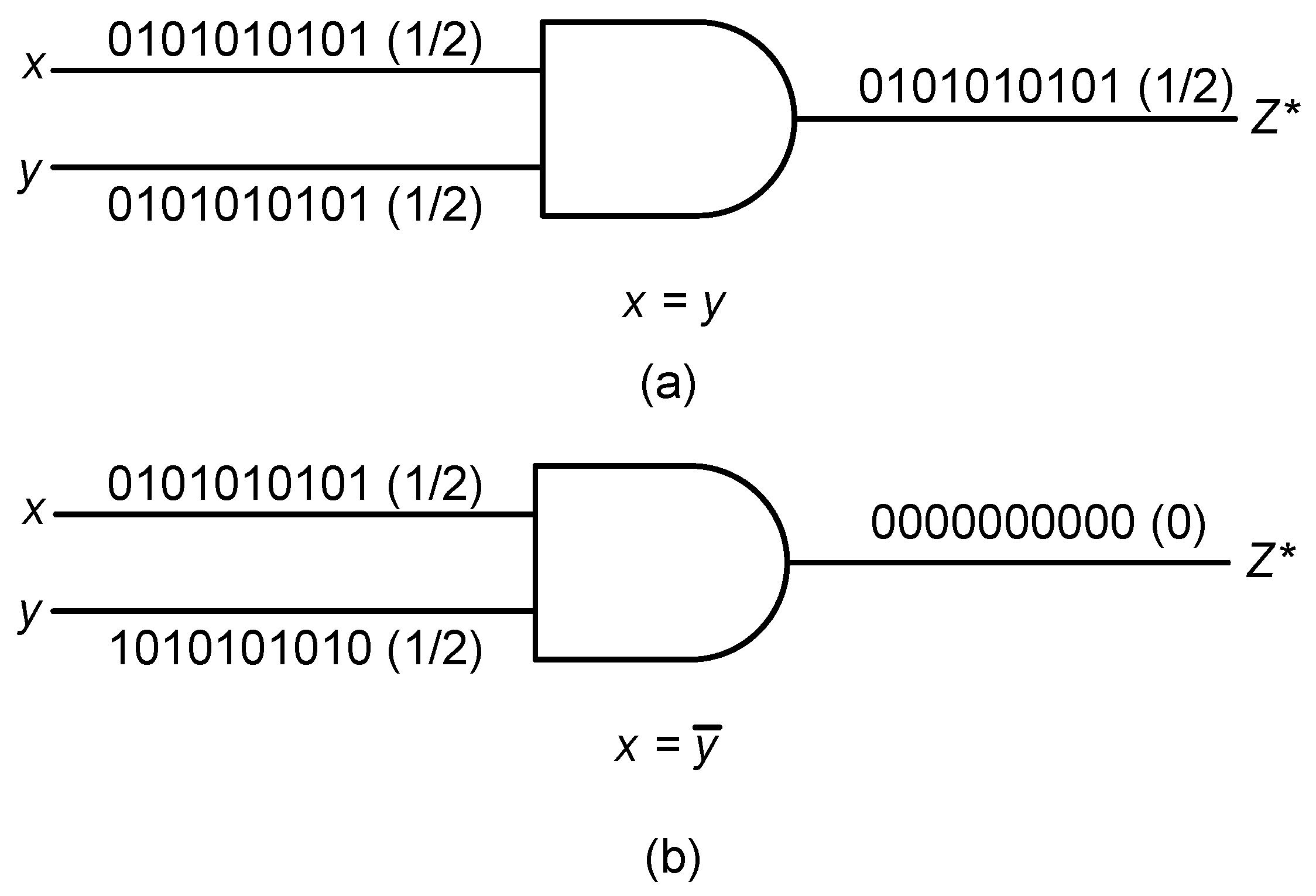
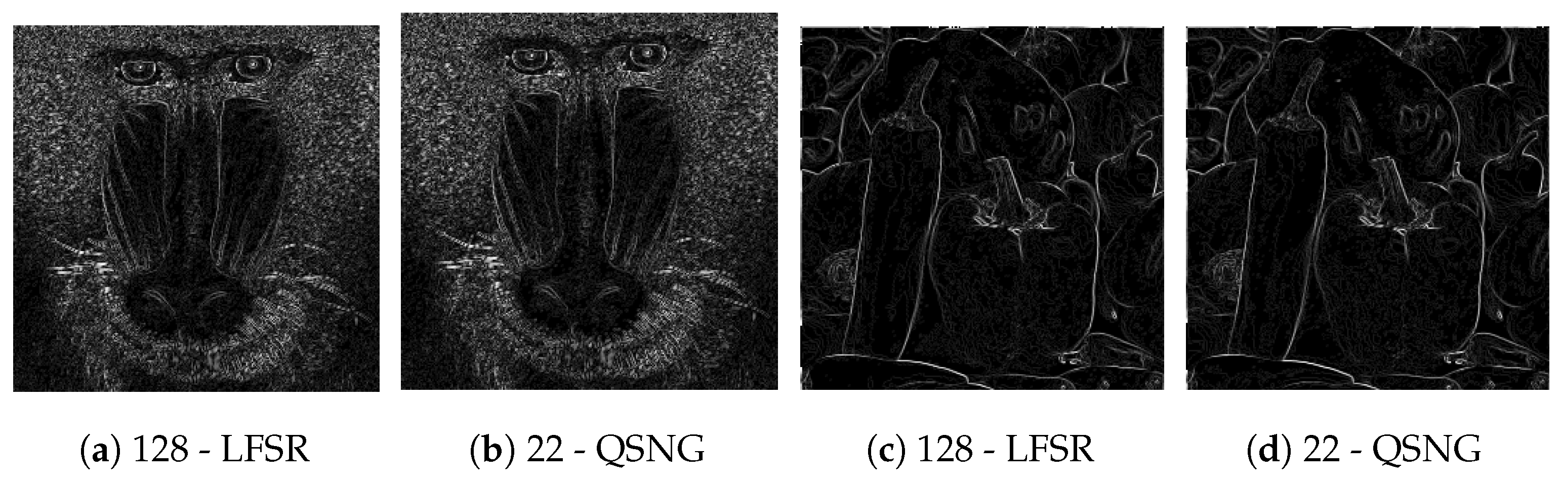
Figure 2 shows two examples where inaccurate results are caused by correlated inputs in the multiplication circuit. This correlation comes from the SNGs, where the SNs generated by SNGs happened to have the same set of sequences of ones and zeros or have some relation among them as shown in Figure 2. This causes inaccuracy in the output generated, so SNGs are always chosen in such a way that they produce uncorrelated SNs. LFSRs are known to be best-suited for SC and have been used for number generation in many SC designs [21]. However, the main disadvantages are the number of SNGs must be higher (i.e., for every independent input, the number of SNGs used increases by one) for uncorrelated inputs and need a longer time to operate for accurate and efficient SC [19].
When the circuit size, power and computation time of SC are considered, the main contributions for these factors to vary significantly are the SNGs. The number of SNGs is proportional to the area of a stochastic circuit, contributing to about 80% of the circuit area. The power consumed by SC mainly depends on the number of clock cycles the circuit uses for computation, which in turn, depends on the SNG properties. The computation time can be limited by SNGs due to their inherent properties such as random number fluctuations. The computation time increases exponentially with the linear increase in accuracy, hence the need to address basic questions such as: What is the minimum number of clock cycles needed to run, so the probability value is represented correctly? What is the effect of random noise fluctuations in a sequence of stochastic operations? Answers to these questions may help in decreasing the computation time drastically. SC has another disadvantage over the binary implementation as all the operations in the SC are single staged; therefore, conventional techniques such as pipelining to improve the throughput cannot be applied [18].
This paper is organized as follows. Section 3 gives the background of the LD sequences and LUT-based method implemented. Section 4 discusses the parallel implementation of SNGs and the different stages used in the parallel implementation of SNGs for parallel stochastic computing. Section 5 discusses the simulation results comparing the proposed SNG with the pseudo-random number generators (LFSRs). An analysis of the convergence rate of the proposed SNG with that of the LFSR is given. A discussion of the application of the proposed serial and parallel SNG in edge detection and the multiplication circuit and the specification of the advantages over the LFSR implementation is given. Finally, Section 6 provides the conclusion.

3. Proposed LUT-Based Method for LD Sequence Generation

In the proposed approach, SNGs are designed to leverage LUTs, which are the distributed memory elements of the FPGAs. The primary focuses of this paper are on decreasing the power consumed, improving the accuracy, reducing the number of random fluctuations and reducing the execution time by parallel implementation using the proposed LUT-based Quasi-SNG (QSNG). FPGAs are the target hardware implemented in this design for their abundant availability of LUTs and their inherent parallel nature. Among various applications, LUTs are used in digital signal processing algorithms, where multiplication is done with a fixed set of coefficients that are already pre-computed and stored in the LUT, so they can be used without computing them each time [22]. The same concept is used in this paper, where pre-computed fixed direction vectors are multiplied with a binary number to get the desired sequence. The LUT-based method is used to develop stochastic bit numbers by using Quasi-Monte Carlo (QMC) methods [23]. The LD sequences in the literature are used to develop these stochastic numbers. The main advantage gained over the use of LFSRs is that LD sequences do not suffer from random fluctuations as the zeros and ones are uniformly spaced [2]. This is unlike LFSRs, where the zero and ones are non-uniformly spaced. The idea behind the LD sequences is to let the fraction of the points within any subset of [ 0 , 1 ) be as close as possible, such that the low-discrepancy points will spread over [ 0 , 1 ) as uniformly as possible, reducing gaps and clustering points. Figure 3 shows the comparison of pseudo-random points (LFSR implementation) and LD points (Sobol sequence) in the unit square. LD points shows even and uniform coverage of the area of interest as shown and are to converge faster when applied to SC.
The widely-used sequences that fall under the LD sequence category are the Halton sequence, Sobol sequence, Faure sequence and Niederreiter sequence [23,25,26]. Generating these sequences is usually software based because the hardware implementation of all these sequences is not suited for SC due to their complexity in construction [2]. This disadvantage of LD sequences is mitigated fully by the proposed LUT-based approach. The main difference in generating the LD sequences lies in the construction of their direction vectors [23]. Each sequence has a specific type of algorithm to compute these, and the uniformity of the sequence depends on the way these direction vectors are computed. In this paper, LUT-based SNGs were designed using three LD sequences including Halton, Sobol and Niederreiter. The digital method was chosen to design these sequences, restricting the base value to binary base two. For a detailed explanation about the sequences mentioned above, refer to [23].
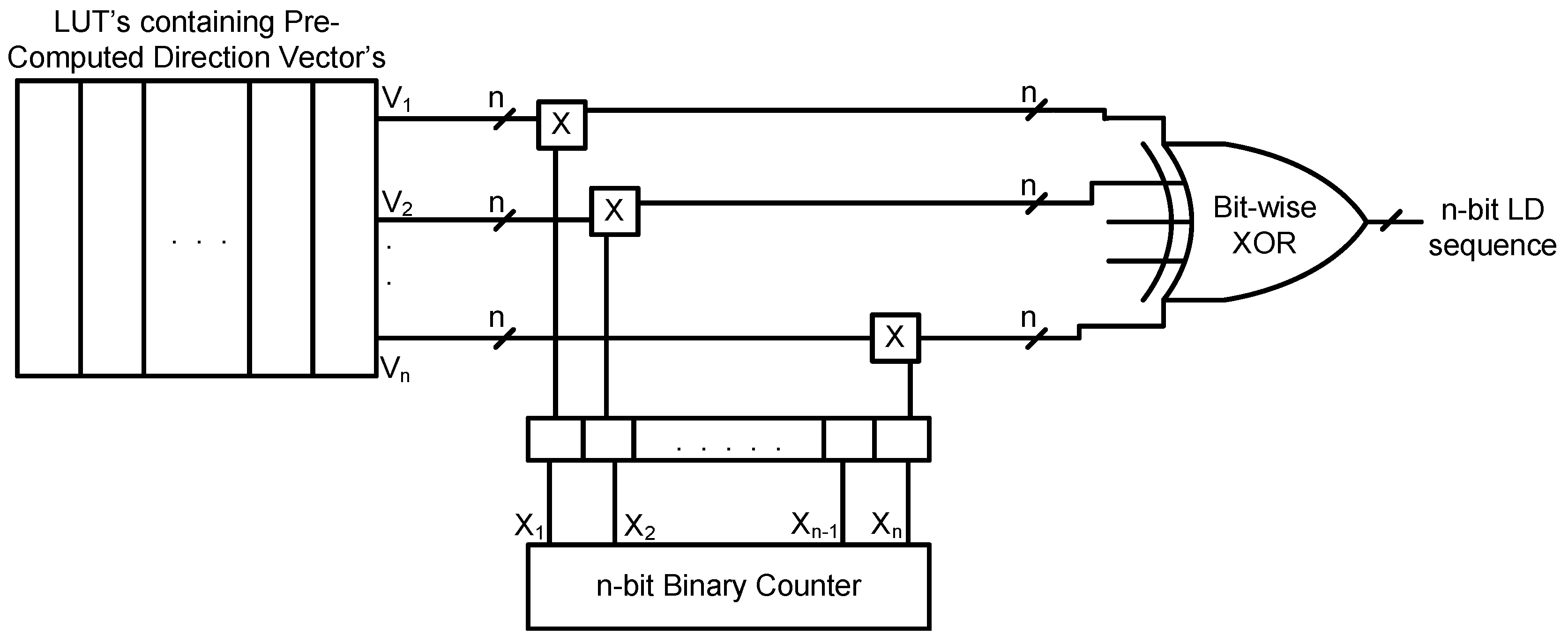
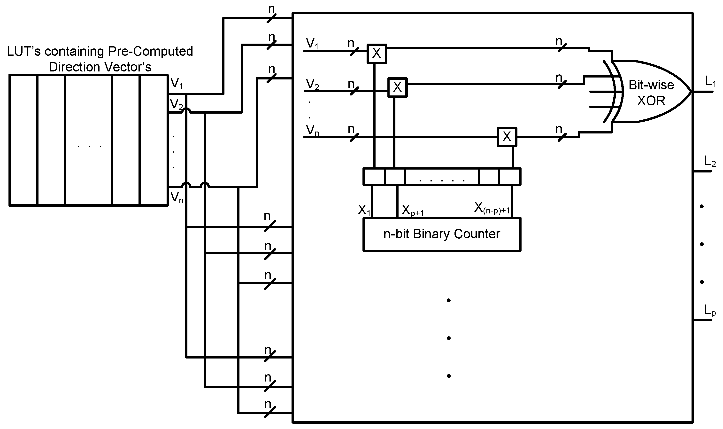
The general structure used for generation of the LD sequence using binary base two is as shown in Figure 4. It contains RAM to store the direction vectors, a multiplication circuit and bit-wise XOR gates. In the multiplication circuit, every bit from the counter output is multiplied by each n-bit direction vector, stored in the RAM, to generate n-bit intermediate direction vectors. These n-bit intermediate direction vectors are then bit-wise XORed (i.e., modulo-two addition) to generate an n-bit LD sequence.
This can be expressed by using a mathematical expression as shown in the equation below [23]:
N = x 1 ( n 1 ) · V 1 x 2 ( n 1 ) · V 2 ,
where ⊕ denotes binary addition or XOR operation, x 1 ( n 1 ) x 2 ( n 1 ) is the binary representation of ( N 1 ) , V 1 , V 2 , V n represents the direction vectors and N represents the N-th number in the respective LD sequence; for example N = 8 represents the eighth number in a Sobol sequence, which is computed by using n direction vectors and an n-bit counter, when Sobol sequence direction vectors are used [23]. Sobol and Niederreiter sequences belong to the general class of digital sequences, and their LD sequence generation can be expressed by the above digital method [25,27]. The Halton sequences belong to the simplest form of LD sequences, and their construction does not have a general form as mentioned above in Equation (1). In the above Equation (1), V 1 , V 2 , V n are called the direction vectors and are defined as the constant values that have to be multiplied with the counter output to generate the desired LD sequence as shown in Figure 4. These values do not change throughout the operation of the circuit; hence, for the generation of Halton LD sequences, defining the direction vectors to fit into the above equation of the general digital method of LD sequence is necessary to generalize the hardware structure for the LD sequences mentioned in the paper.
Halton sequences are defined as the generalized form of van der Corput sequences, which use a distinct prime base for every dimension. The k t h Halton point H ( k ) is defined as H ( k ) = i = 0 a i ( k 1 ) b i 1 [26]. Upon closer inspection of the summation, we define a i ( k 1 ) to be nothing, but the base b representation of k 1 , and b i 1 is the base b term, which has to be multiplied with a i ( k 1 ) for the generation of each sequence depending on the value of k. The term b i 1 is a constant term, and the value does not change with the change in the value of k; hence, these terms are defined as direction vectors and fit into the general form represented above to generate an LD sequence by choosing the base b = 2 . Sobol and Niederreiter sequences have specific algorithms to calculate the direction vectors that fit into Equation (1) to generate the LD sequence. In this paper, algorithms reported in papers [25] and [23] are used to pre-calculate direction vectors. An important point to note in this implementation is that the number of sequences generated is limited by using only R base b direction vectors of R bits, which are capable of representing a value of b R 1 in base b [23]. For example, to generate a stochastic bit length of 256, the generation of only initial 256 LD sequences is required. For this process, eight-bit length direction vectors, which are capable of generating an eight-bit length LD sequence every clock cycle, are needed. The maximum value they can represent is b 8 1 = 255 , limiting the size of the counter. For the above 256 initial sequences, an eight-bit counter is needed to count from zero to 255.
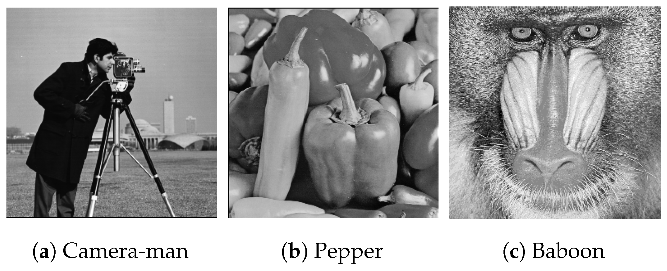
After generation, the LD sequence numbers are sent to the comparator where they are compared with the input value to generate an equivalent stochastic number. The size of the proposed SNG depends on the stochastic bit length L of the circuit, as well as the number of inputs to the stochastic circuit. For a stochastic bit length of 256, it is necessary to use an eight-bit binary counter and a memory space of 64 bits to store eight direction vectors each of an eight-bit length. Independent stochastic inputs require different direction vectors; as the number of independent stochastic inputs increases, the memory space required to store these direction vectors increases. LUT-based SNGs were implemented for 256-, 512-, 1024- and 2048-bit lengths on the Xilinx Virtex 4-SFFPGA (XC4VLX15) device and synthesized using the Xilinx ISE tool. In this paper, a general form of implementation was presented, and further optimization of the circuit has been left for a future study. Table 2 clearly shows that the LD sequence generators make use of more hardware when compared to the LFSRs, but the convergence and the accuracy obtained from LD sequences are superior enough to justify this extra hardware utilization (explained in the following sections).

4. Parallel Implementation of Proposed SNGs for SC

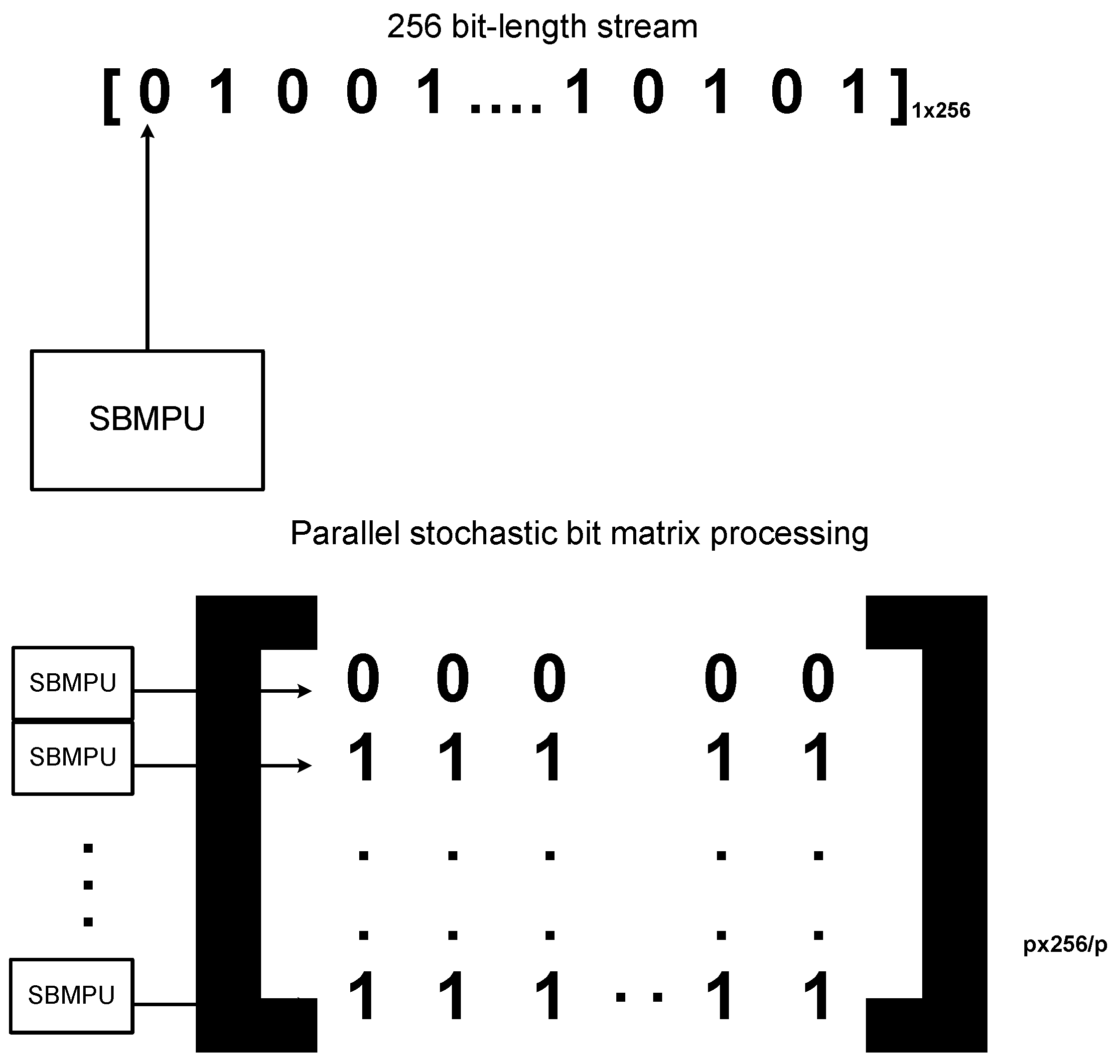
The proposed parallel implementation of the SNGs was designed to generate LD sequence numbers in parallel. These LD sequence numbers generated in parallel were used to generate stochastic bits in parallel. These stochastic numbers, generated in parallel, are termed as Stochastic Bit Vectors (SBVs), and the parallel processing used to generate the sequence is termed as Stochastic Bit Matrix (SBM) processing. Consider a 256-bit length stochastic bit matrix, this design generates p initial bits every clock cycle of the SBM, instead of generating one bit of the SBM. This is shown in a vector form in Figure 5, which shows that for one stochastic bit generation using a single SBM Processing Unit (SBMPU), 256 clock cycles are needed to generate a 256-bit length SBM. By duplicating p SBMPUs in parallel, it is also possible to generate p stochastic bits of the SBM in just one clock cycle. Hence, 256 / p clock cycles are needed for generating a 256-bit length, thus saving the execution time of the operation as p increases.
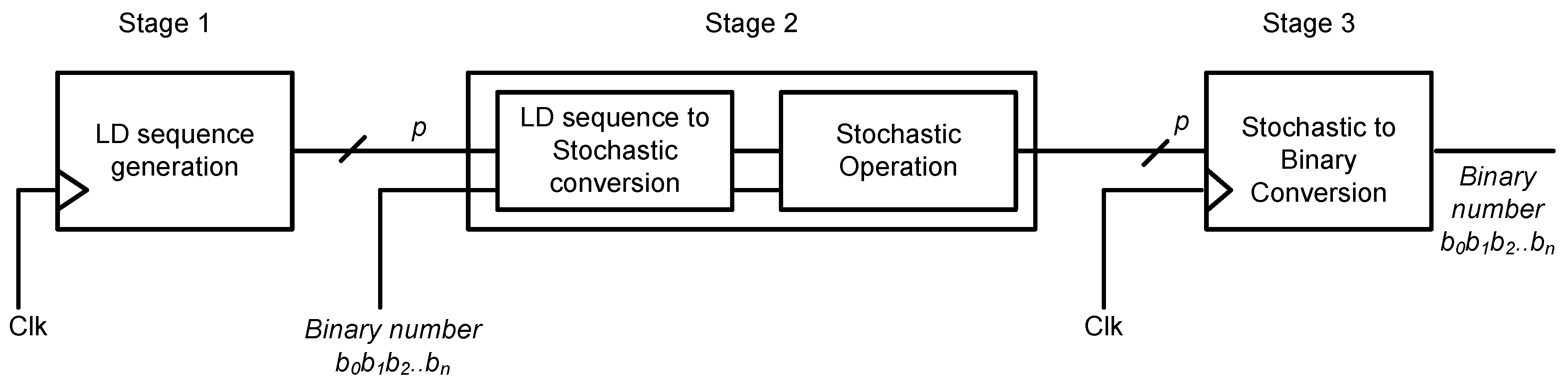
The structure of the parallel implementation of the circuit is shown in Figure 6. The parallel implementation of the proposed SNGs is done in three stages. The first stage is where the LD sequence numbers are generated in parallel. The second stage is where the stochastic bit streams are generated in parallel using comparators and sent to the stochastic circuit for SC. Finally, the third stage is where the stochastic output is converted back to a binary output by counting the number of ones. A combinational circuit is implemented for the conversion of stochastic to binary number by counting the number of ones in the SN by making use of the Hamming weight counter principle [28].

4.1. First Stage

The first initial p LD sequence numbers are generated in parallel depending on the degree of parallelism. The general structure of the implementation is as shown in Figure 7. Here, the entire structure is not duplicated, but the part of the SNG that generates the LD sequence number is duplicated to reduce the area overhead. The degree of parallelism determines the amount of hardware utilized. Counters, which follow a specific sequence of counting, are used to implement the SNGs in parallel. For example, to generate the first initial eight sub-sequences in parallel of a 256-bit stream length, use eight eight-bit counters, which count by eight. The first counter follows the sequence 0 , 8 , 16 , 32 , and the second counter follows the sequence 1 , 9 , 17 , 33 in the same way as the eighth counter follows the sequence 7 , 15 , 31 . Therefore, in the first clock cycle, the eight counters hold the value from zero to seven, which means that the first eight LD sequence numbers are generated in parallel. In the second clock cycle, the counters are incremented by one to hold the value eight to 15, and the next eight LD sequence numbers are generated. These generated sequences are then sent to the parallel comparator units where they are compared with the input probability value to generate the stochastic bits in parallel. This implementation generates a sequence for a single input in parallel. For multiple inputs, different direction vectors can be used, while the circuit for the generation of the LD sequence is the same.

4.2. Second Stage

The second stage consists of the generation of the stochastic bit stream and the stochastic operation. For the generation of the stochastic bit stream, the LD sequences generated in parallel are sent to the comparators, which are also in parallel, such that multiple sequences are compared simultaneously to generate a stochastic bit stream in parallel. For example, to generate eight-bits of the stochastic bit stream, use eight comparators where each sequence is compared with the binary probability value to generate the first eight bits of the SN at the same time. This is termed as eight-bit SBV generation using an eight SBM processing in one clock cycle by replicating the SBM circuit eight times. Similarly, to generate 16 SBV’s, 16 SBM processing is done in one clock cycle replicating the SBM circuit 16 times.
The SBM processing circuit involves only that part of the LD sequence generator capable of generating the sequence (i.e., the multiplication and the bit-wise XOR structure) and an LD sequence to the stochastic conversion unit (i.e., comparator); the LUTs used are shared among the parallel SBM processing units as they are constant values that do not change during the execution cycle. The generated stochastic bits by SBM processing are then sent for computation and then to the stochastic to binary conversion stage for final output. See Figure 8 for the parallel structure of the stochastic bit stream generators. The number of comparators used depends on the degree of parallelism implemented. Hence, the degree of parallelism determines the hardware utilized.

4.3. Third Stage

The final stage in a stochastic computation is to create the binary output, which is generated by using STB conversion units, which are comprised of a counter that counts the number of ones in the stochastic bit-stream. If the output stochastic bits generated are eight bits per clock cycle, it is necessary to count the number of ones in the initial eight-bits within one clock cycle; this is not possible by using a single counter circuit with the same clock period. In this paper, an STB conversion unit is used that converts the parallel stochastic output into a binary number by using simple adder circuits. This circuit can count the number of ones in a parallel bit stream by using the Hamming weight counter principle [
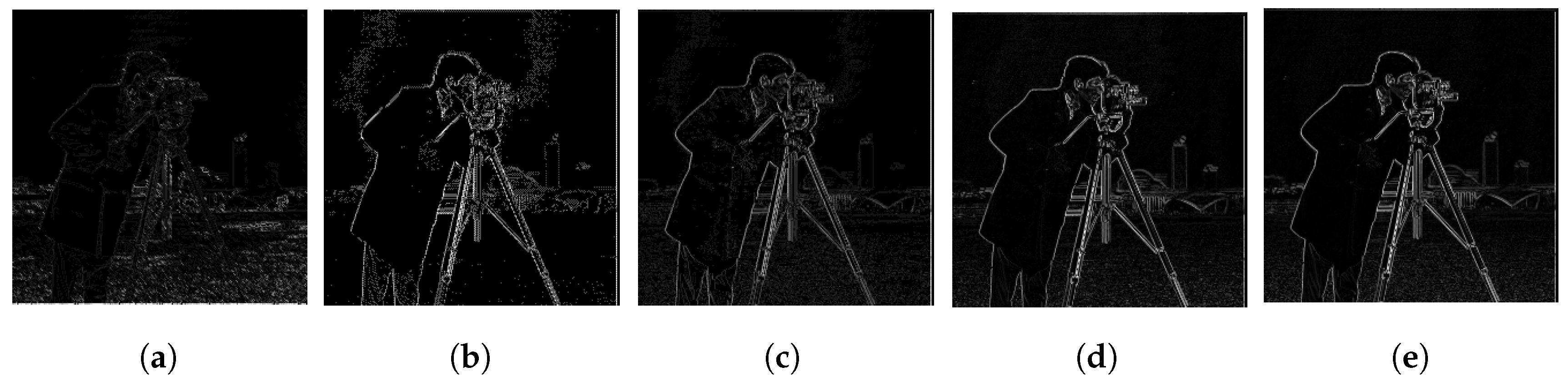
28]. The structure of the STB conversion unit for counting the number of ones in eight parallel stochastic bits of a 256-bit stream length consists of four half adders, two two-bit adders, a three-bit adder, an eight-bit register and a four-bit adder. An eight-bit register is used to store the previous count value, and it is updated every clock cycle with the new value (i.e., the number of ones in the stochastic bit stream). To count the number of ones in 16 stochastic bits of a 256-bit stream length, eight half adders, four two-bit adders, two three-bit adders, an eight-bit register and an eight-bit adder are required. Therefore, the size of the STB conversion unit increases with the number of parallel bits generated. The scalability issue of the STB conversion unit may not be a major concern as the proposed approach mainly targets image processing applications where the word length for many operations is less than 16 bits. The next section presents the simulation results of both the parallel and the serial implementation of the LUT-based LD sequence SNGs.

5. Simulation Results

Simulation results are comprised of both serial and parallel implementation of the LUT-based LD sequence SNGs. All the circuits have been implemented on a Xilinx Virtex 4 SF FPGA (XC4VLX15) device and synthesized using the Xilinx ISE 12.1 design suite, with the minimum area and power reduction as optimization goals. The accuracy of the sequence generator proposed in this work is compared with that of the pseudo-random number generator (LFSR implementation). The results demonstrate that the proposed SNG generators have better convergence when compared with LFSRs. The LUT-based SNGs are used in image processing and arithmetic application of SC (i.e., edge detection and multiplication) to compare the results with the LFSR-based SNGs.

5.1. Edge Detection

The proposed SNGs were tested with stochastic edge detection circuit for eight-bit grayscale images i.e., each pixel was represented using a stochastic bit-length of 256 bits. In this work, an edge detection circuit has been implemented using the stochastic circuit described in [5] as shown in Figure 1g. This circuit is implemented based on Robert’s cross algorithm. The test images selected for implementing the edge detection algorithm are shown in Figure 9. The pixel values of the images were extracted using MATLAB and were given as the eight-bit binary input to the proposed SNGs. The outputs from the proposed SNGs were given to the stochastic edge detection circuit, and the outputs extracted from the post synthesis simulation results were processed in MATLAB. To evaluate the convergence rate and quality of the image generated by the proposed SNGs, MAE (Mean Absolute Error) and PSNR (Peak Signal-to-Noise Ratio) were calculated for the output edge detected image every clock cycle, and the results were compared to the output generated by using pseudo-random number generators (LFSRs).
PSNR is commonly adopted in the image processing field to quantify the acceptability of erroneous or noisy images [29]. The PSNR value (usually in the unit of dB) can indicate the similarity of two different images. Here, the edge detection image generated by running for 256 clock cycles and the edge detection image generated by running for q clock cycles are used to compute the corresponding PSNR value. The q value is defined as the number of clock cycles needed to output a satisfactory result within an absolute error of less than 0.01 between the actual and the predicted value. PSNR value can be calculated by the equation below [29].
P S N R = 10 · log 10 M A X I 2 M S E ,
where M S E = 1 m n i = 0 m 1 j = 0 n 1 | I ( i , j ) K ( i , j ) | 2 is the mean square error of the error-free and the erroneous image, M A X I is the maximum image pixel value (e.g., 255 in the eight-bit grayscale image), m and n represent the width and height of the target image in terms of the number of pixels and I ( i , j ) and K ( i , j ) represent the pixel values of the error-free image and the erroneous/noisy image, respectively. From Equation (2), when the erroneous image is more similar to the original one, a smaller MSE and a higher PSNR value will be obtained.
The MAE value is calculated every clock cycle to determine the q clock cycles needed to output a satisfactory result within an absolute error of 0.01 . It is defined as the average of the absolute difference between the actual value and the predicted value. It can be calculated by using the equation below [29].
M A E = 1 m n i = 0 m 1 j = 0 n 1 | I ( i , j ) K ( i , j ) | ,
where m and n represent the width and height of the target image in terms of the number of pixels, I ( i , j ) represent the pixel values of the edge detection image generated by running for 256 clock cycles (actual value) and K ( i , j ) represent the pixel values of the edge detection image generated by running for r clock cycles (predicted value) where r varies from one to 255, respectively. When MAE equals 0.01 , r equals q.
Initial analysis was done on the open-source benchmark image “Camera-man” shown Figure 9a. It was found that the edge detection circuit using the pseudo-random generator as an SNG took 128 clock cycles to output an absolute error of less than 0.01 as compared to 22 clock cycles required for an LUT-based QSNG. A similar kind of analysis on test images “Pepper” and “Baboon” resulted in the same results. Figure 10, Figure 11 and Figure 12 show the edge detection results for the test images. For Figure 12, the results were not shown for different clock cycles to reduce the space. Table 1 shows the PSNR and MAE values for the test images at different clock cycles. From the table, it can be concluded that the proposed SNGs show a better convergence at a faster rate as compared to pseudo-random generators with an acceptable image quality [29].

5.2. Multiplication

The stochastic multiplication circuit as shown in Figure 1a is being implemented for an eight-bit binary input number using both pseudo-random and LD sequence generators. The average number of clock cycles needed to generate a satisfactory result per input is calculated by giving a random set of 256 input values (xand y) and calculating the average number of clock cycles needed to generate an output with an absolute error of less than 0.01 . For the multiplication circuit, the MAE is mathematically represented as | P z - P z | where, P z is the actual output value and P z is the predicted output value after stochastic computation. It turns out that for LFSR (pseudo-random number generator) as an SNG, the average number of clock cycles needed is 512, and for LUT-based QSNG it is 54 clock cycles only.

5.3. Hardware Utilization

Table 2 shows the comparison of LUT-based QSNG (LD sequence) and LFSR-based (pseudo-random sequence) SNG in terms of resource utilization, average run-time and the average power consumed for edge detection and multiplication circuits. In this paper, average run-time is calculated by multiplying the clock period of the circuit by the average number of clock cycles needed to generate a satisfactory output, which is defined as an output with an MAE of less than 0.01 . The average power is calculated for the average run-time in both approaches. The numbers are estimated values based on the implementation results on the Xilinx Virtex 4 SF FPGA (XC4VLX15) device. From Table 2, the average run time and the power consumed are reduced by 4.5 -times for the multiplication circuit and 3.5 -times for the edge detection circuit. Though the area occupied by the LUT-based QSNG is more as compared to the LFSR-based SNG when the convergence power of the LD sequence is considered acceptable, the results can be achieved at a much faster rate and with a considerable power reduction as shown in the Table 2. For applications that have a trade-off of area for speed and power consumed, the proposed LUT-based QSNG would be very beneficial. The proposed approach is a better low-power design as compared to the conventional stochastic approach.
The hardware utilization of the parallel implementation of edge detection and multiplication circuits is shown in Table 3. Since it is clear from the previous results that the convergence power of LD sequence generators is better than the LFSRs for the same circuit implementation, LD sequences generators’ hardware utilization can be reduced by restricting it to the generation of initial sub-sequences rather than complete sets of sequences. The throughput of the system can be increased drastically by using the proposed parallel implementation. For instance, the proposed serial implementation of the edge detection circuit reduces the computation time by a factor of 35-times; if the same circuit is realized in parallel say with a degree of parallelism of four, we need to run it for just six clock cycles to generate the initial sub-sequence of 24 LD sequences, which would be enough to achieve an acceptable output. On the other hand, for the LFSR-based SNG, we need to run it for 32 clock cycles to generate the initial 128 sequences, which are capable enough to output an acceptable image. The computation time is decreased by a factor of four here suggesting that the throughput of the system has increased. Therefore, by using the proposed SNGs, both the execution time and power consumed can be reduced while achieving a higher throughput by implementing them in parallel.

6. Conclusions

This paper has introduced a novel construction method to realize QSNGs on FPGA using LUTs. The FPGA’s superior reconfigurability was leveraged advantageously for parallel implementation of a stochastic circuit that outperforms the conventional LFSR-based stochastic circuit approach in terms of convergence, power consumed and accuracy. Simulation results suggest that both computation time and power consumed can be saved up to 3.5 -times in the edge detection circuit and up to 4.5 -times in the multiplication circuit as compared to the conventional stochastic approach. Further, extensive simulation results justify that for faster (higher throughput) and more accurate computation with a low-power consumption, making use of FPGA-based parallel quasi-stochastic computing is a better option. The future scope of this work is to optimize the LD sequence generator circuit with a combinational logic to generate the LD sequence to reduce the area occupied.

Author Contributions

All authors contributed equally to this work.

Conflicts of Interest

The authors declare no conflict of interest.

References

  1. Sobol, I.M. Uniformly distributed sequences with an additional uniform property. USSR Comput. Math. Math. Phys. 1976, 16, 236–242. [Google Scholar] [CrossRef]
  2. Alaghi, A.; Hayes, J.P. Fast and accurate computation using stochastic circuits. In Proceedings of the Conference on Design, Automation & Test in Europe Conference and Exhibition (DATE), European Design and Automation Association, Dresden, Germany, 24–28 March 2014; p. 76. [Google Scholar]
  3. Gaines, B.R. Stochastic computing. In Proceedings of the 18–20 April 1967, Spring Joint Computer Conference, Atlantic City, NJ, USA, 18–20 April 1967; pp. 149–156. [Google Scholar]
  4. Gaines, B. Stochastic computing systems. In Advances in Information Systems Science; Springer: Berlin, Germany, 1969; pp. 37–172. [Google Scholar]
  5. Alaghi, A.; Li, C.; Hayes, J.P. Stochastic circuits for real-time image-processing applications. In Proceedings of the 50th Annual Design Automation Conference, Austin, TX, USA, 29 May–7 June 2013; p. 136. [Google Scholar]
  6. Naderi, A.; Mannor, S.; Sawan, M.; Gross, W.J. Delayed stochastic decoding of LDPC codes. IEEE Trans. Signal Process. 2011, 59, 5617–5626. [Google Scholar] [CrossRef]
  7. Aliee, H.; Zarandi, H.R. Fault tree analysis using stochastic logic: A reliable and high speed computing. In Proceedings of the 2011 Proceedings-Annual Reliability and Maintainability Symposium (RAMS), Lake Buena Vista, FL, USA, 24–27 January 2011; pp. 1–6. [Google Scholar]
  8. Li, P.; Lilja, D.J. Using stochastic computing to implement digital image processing algorithms. In Proceedings of the 2011 IEEE 29th International Conference on Computer Design (ICCD), Amherst, MA, USA, 9–12 October 2011; pp. 154–161. [Google Scholar]
  9. Chang, Y.N.; Parhi, K. Architectures for digital filters using stochastic computing. In Proceedings of the 2013 IEEE International Conference on Acoustics, Speech and Signal Processing (ICASSP), Vancouver, BC, Canada, 26–31 May 2013; pp. 2697–2701. [Google Scholar]
  10. Saraf, N.; Bazargan, K.; Lilja, D.J.; Riedel, M.D. IIR filters using stochastic arithmetic. In Proceedings of the 2014 Design, Automation and Test in Europe Conference and Exhibition (DATE), Dresden, Germany, 24–28 March 2014; pp. 1–6. [Google Scholar]
  11. Li, P.; Lilja, D.J. Accelerating the performance of stochastic encoding-based computations by sharing bits in consecutive bit streams. In Proceedings of the 2013 IEEE 24th International Conference on Application-Specific Systems, Architectures and Processors (ASAP), Washington, DC, USA, 5–7 June 2013; pp. 257–260. [Google Scholar]
  12. Ichihara, H.; Ishii, S.; Sunamori, D.; Iwagaki, T.; Inoue, T. Compact and accurate stochastic circuits with shared random number sources. In Proceedings of the 2014 32nd IEEE International Conference on Computer Design (ICCD), Seoul, Korea, 19–22 October 2014; pp. 361–366. [Google Scholar]
  13. Alaghi, A.; Hayes, J.P. A spectral transform approach to stochastic circuits. In Proceedings of the 2012 IEEE 30th International Conference on Computer Design (ICCD), Montreal, QC, Canada, 30 September–3 October 2012; pp. 315–321. [Google Scholar]
  14. Alaghi, A.; Hayes, J. STRAUSS: Spectral Transform Use in Stochastic Circuit Synthesis. IEEE Trans. Comput. Aided Des. Integr. Circuits Syst. 2012, 34, 1770–1783. [Google Scholar] [CrossRef]
  15. Chen, T.H.; Hayes, J.P. Equivalence among Stochastic Logic Circuits and its Application to Synthesis. IEEE Trans. Emerg. Top. Comput. 2016. [Google Scholar] [CrossRef]
  16. Kwok, S.H.; Lam, E.Y. FPGA-based high-speed true random number generator for cryptographic applications. In Proceedings of the 2006 IEEE Region 10 Conference on TENCON 2006, Hong Kong, China, 14–17 November 2006; pp. 1–4. [Google Scholar]
  17. Majzoobi, M.; Koushanfar, F.; Devadas, S. FPGA-Based True Random Number Generation Using Circuit Metastability with Adaptive Feedback Control. Cryptogr. Hardw. Embed. Syst. 2011, 6917, 17–32. [Google Scholar] [Green Version]
  18. Moons, B.; Verhelst, M. Energy-Efficiency and Accuracy of Stochastic Computing Circuits in Emerging Technologies. IEEE J. Emerg. Sel. Top. Circuits Syst. 2014, 4, 475–486. [Google Scholar] [CrossRef]
  19. Alaghi, A.; Hayes, J.P. Survey of stochastic computing. ACM Trans. Embed. Comput. Syst. 2013, 12. [Google Scholar] [CrossRef]
  20. Manohar, R. Comparing Stochastic and Deterministic Computing. IEEE Comput. Archit. Lett. 2015, 14, 119–122. [Google Scholar] [CrossRef]
  21. Gupta, P.; Kumaresan, R. Binary multiplication with PN sequences. IEEE Trans. Acoust. Speech Signal Process. 1988, 36, 603–606. [Google Scholar] [CrossRef]
  22. Thomas, D.B.; Luk, W. The LUT-SR family of uniform random number generators for FPGA architectures. IEEE Trans. Very Large Scale Integration (VLSI) Syst. 2013, 21, 761–770. [Google Scholar] [CrossRef]
  23. Bratley, P.; Fox, B.L.; Niederreiter, H. Implementation and tests of low-discrepancy sequences. ACM Trans. Model. Comput. Simul. 1992, 2, 195–213. [Google Scholar] [CrossRef]
  24. Wikipedia. Low-Discrepancy Sequence. Available online: www.en.wikipedia.org/wiki/Low-discrepancy_sequence (accessed on 9 April 2017).
  25. Sobol, I. On the distribution of points in a cube and the approximate evaluation of integrals. USSR Comput. Math. Math. Phys. 1967, 7, 784–802. [Google Scholar] [CrossRef]
  26. Halton, J.H. On the efficiency of certain quasi-random sequences of points in evaluating multi-dimensional integrals. Numer. Math. 1960, 2, 84–90. [Google Scholar] [CrossRef]
  27. Niederreiter, H. Point sets and sequences with small discrepancy. Mon. Math. 1987, 104, 273–337. [Google Scholar] [CrossRef]
  28. Parhami, B. Efficient hamming weight comparators for binary vectors based on accumulative and up/down parallel counters. IEEE Trans. Circuits Syst. II Express Briefs 2009, 56, 167–171. [Google Scholar] [CrossRef]
  29. Hsieh, T.Y.; Peng, Y.H.; Ku, C.C. An Efficient Test Methodology for Image Processing Applications Based on Error-Tolerance. In Proceedings of the 2013 22nd Asian Test Symposium, Jiaosi Township, Taiwan, 18–21 November 2013; pp. 289–294. [Google Scholar]
Figure 1. Basic circuits used in stochastic computation [18]. UP, unipolar; BP, bipolar.
Jlpea 07 00029 g001
Figure 2. (a) Correlation effect in an AND gate (multiplier circuit in Stochastic Computing (SC)) when both bit streams are the same; (b) correlation effect when both bit streams are inverse of each other.
Jlpea 07 00029 g002
Figure 3. Distribution of pseudo-random points (top) and Low-Discrepancy (LD) points (bottom) in the unit square [24].
Jlpea 07 00029 g003
Figure 4. Basic block diagram of the proposed Quasi-Stochastic Number Generator (QSNG).
Jlpea 07 00029 g004
Figure 5. Parallel stochastic bit matrix processing. SBMPU, Stochastic Bit Matrix Processing Unit.
Jlpea 07 00029 g005
Figure 6. Three stages of parallel implementation.
Jlpea 07 00029 g006
Figure 7. First stage of LD sequence generation.
Jlpea 07 00029 g007
Figure 8. Second stag: LD to stochastic bit conversion.
Jlpea 07 00029 g008
Figure 9. Test images for edge detection.
Jlpea 07 00029 g009
Figure 10. Edge detection using Linear Feedback Shift Registers (LFSRs): (a) eight clock cycles; (b) 22 clock cycles; (c) 64 clock cycles; (d) 128 clock cycles; (e) 256 clock cycles.
Jlpea 07 00029 g010
Figure 11. Edge detection using LD sequence generators: (a) eight clock cycles; (b) 22 clock cycles; (c) 64 clock cycles; (d) 128 clock cycles; (e) 256 clock cycles.
Jlpea 07 00029 g011
Figure 12. Edge detection results from LFSR and QSNG. Note: the 22 clock-cycle QSNG results are comparable to the 128 clock-cycle LFSR results.
Jlpea 07 00029 g012
Table 1. Table showing the PSNR and MAE values for test images.
Test-ImageSequenceClock CyclesPSNR (dB)MAE
822.990.375
Camera-manLD Sequence2230.860.0101
6434.310.005
12842.010.002
819.680.1466
Pseudo-random sequence2221.230.1164
6426.310.0394
12836.210.0101
824.840.04
BaboonLD Sequence2229.610.0084
6434.840.0046
12840.010.002
820.680.1383
Pseudo-random sequence2221.360.1264
6428.310.02
12833.210.0101
826.710.0321
PepperLD Sequence2231.060.0102
6435.000.0046
12842.220.0025
818.680.1766
Pseudo-random sequence2220.460.1464
6424.350.0466
12832.220.0079
Table 2. Table showing the resource utilization for the serial implementation.
SequenceApplication# of Occupied
Slices
Max Freq
(MHz)
Average Run-Time
(ns)
Average Power
(uW)
LD SequenceMultiplication70224.30240.70.3
Edge detection140222.301000.12
Pseudo-RandomMultiplication17458.321117.11.34
Edge detection48374.523410.41
Table 3. Resource utilization comparison for the parallel implementation.
SequenceApplicationDegree of ParallelismSlices
4537
LD SequenceEdge-Detection81069
162125
4104
LD SequenceMultiplication8199
16394
4190
Pseudo-RandomEdge-Detection8382
16767
467
Pseudo-RandomMultiplication8134
16262

