Estimation of Nearshore Wind Conditions Using Onshore Observation Data with Computational Fluid Dynamic and Mesoscale Models

Abstract

This study aimed to establish numerical models to replicate wind conditions for nearshore waters, sensitive to onshore topography, and to compare the characteristics of computational fluid dynamic (CFD) and mesoscale models. Vertical Doppler light detection and ranging (LiDAR) observation data were measured at an onshore site, which showed that wind conditions were affected by thermodynamic phenomena, such as land and sea breeze, and dynamical effects from neighboring onshore topography. The estimation accuracy of the CFD model depended on the height of the LiDAR data input. A height close to the target, such as the hub height of wind turbines, seemed appropriate as input data, considering that the accuracy of the wind speed shear replicated in a CFD numerical model may be uncertain. The mesoscale model replicated the wind through the thermodynamic effect and reliably estimated wind speed over nearshore waters without observation correction. Larger estimation errors were detected in the CFD model than in the mesoscale model, as the former could not account for thermodynamic effects. Wind conditions in water areas near complex coastlines may also be formed by thermodynamic factors, making analysis using a mesoscale model advantageous.

1. Introduction

An accurate offshore wind resource assessment is crucial for implementing offshore wind energy projects. As offshore wind energy development in Japan is still at an early stage, development is expected to start in nearshore and shallow waters, i.e., areas within 5 km from the coast. In Japan, most offshore wind turbines are located at nearshore areas (e.g., Choshi and Kita-Kyushu), and several more are planned [1,2]. It is thus necessary to establish a method for the accurate estimation of nearshore wind conditions.

The best estimation method is based on in situ observations with a meteorological mast; however, constructing an offshore meteorological mast is both costly and difficult at the planning stage [3]. More recently, however, remote sensing measurements, such as Doppler light detection and ranging (LiDAR), a technology that utilizes the Doppler shift of backscattered laser energy to estimate the wind speed within a volume of air, have been found to be highly reliable for wind resource assessment [4,5]. Various types of LiDAR can be used for wind measurement, the most common of which is vertical LiDAR, a technique capable of taking measurements at heights of at least 200 m. Scanning or floating LiDAR is expected to be an inexpensive method compared with an offshore meteorological mast for nearshore and offshore sites [6]. However, LiDAR has a limited track record compared to meteorological masts. The current guidelines for wind resource assessment are therefore based on measurements using a meteorological mast [7,8]. More field experiments under different environmental conditions are required before practical application can be realized.

Nearshore wind conditions may be estimated from the coast. A simple and inexpensive method is to measure wind conditions at the coastline using a met-mast or vertical LiDAR, followed by the application of a numerical computational fluid dynamic (CFD) model or mesoscale model. CFD models, such as the microclimate analysis system for complex terrain (MASCOT) [9,10] and RIAM-COMPACT [11], are generally used in non-linear flow simulations for wind farms in Japan, as these models can effectively replicate wind flow, even over complex terrains.

Developed for weather forecasting, the mesoscale model replicates wind and general atmospheric conditions. However, it is less reliable in replicating wind conditions at sites with complex terrain. The mesoscale model has been frequently applied in offshore wind resource assessments in Europe, where most offshore wind farms are located far from the coasts and wind conditions are not greatly affected by onshore terrain [12,13,14,15,16]. Meanwhile, observation results over nearshore waters in Japan showed that the winds are affected by the terrain, especially when the wind flows from land to sea [17]. The surrounding environment governing wind conditions in Japan substantially differs from the offshore site environments in European seas, such as the North Sea and the Baltic Sea.

The Weather Research and Forecasting model (WRF) [18], the most common mesoscale model, has been used to produce wind information for the new Japanese offshore wind resource map (NeoWins) [19]. The accuracy of the wind speed has been examined using wind turbine hub height measurements from three meteorological masts and a wind LiDAR at four coastal and nearshore sites [20,21]. The accuracy at the four sites was reported as within ±5% for the annual mean wind speed at a hub height. However, the result estimated by the WRF may have a bias exceeding 10% in other areas, with a positive bias, especially those in the vicinity of coastlines at lower altitudes on land and over coastal waters closer to the coastline [22,23,24].

Therefore, an appropriate numerical simulation should be selected for estimation in nearshore waters, where land affects wind conditions. Linear models (such as WAsP [25]), mesoscale models (such as WRF), CFD models, and even coupling methods of these simulations have been proposed for wind resource modeling. Although the accuracy of these methods has been verified, most methods are only suitable for complex terrain [26,27] and coastal areas [28,29]. Previously [30], wind speed profile assessments of an offshore site were compared using WAsP and the mesoscale model MM5 (fifth-generation Penn State/NCAR mesoscale model) [31]. The results of the WAsP method largely depended on the measurement station used as a reference, whereas those of the MM5 were highly accurate, even without measurement data.

To date, there are no experimental studies that compare the features of CFD and mesoscale models in nearshore waters, where wind conditions may be affected by onshore terrain. Moreover, there is insufficient technical knowledge for the selection of the appropriate numerical model. The number of wind projects in offshore areas near complex onshore topography and coastlines is expected to increase, as exemplified by offshore wind farms planned for development in Japan.

Therefore, this study aimed to compare numerical simulation estimates for offshore areas with complex wind characteristics. In particular, the CFD and mesoscale models were used to elucidate the features of wind condition estimates for nearshore waters, and their accuracy was determined using data from a 3-month observation campaign performed in the coastal area of Shirahama, Wakayama Prefecture, Japan. The nearshore area, located near such complex topography and with an intricate coastline, is a typical offshore wind area influenced by land.

This paper presents the methods of both observation and numerical simulations in Section 2. Section 3 presents the results of the comparison of the numerical simulation estimates and observation data, and discusses the factors causing the differences between the models and the observation. Section 4 provides a summary of the study.

2. Observation Data and Methods

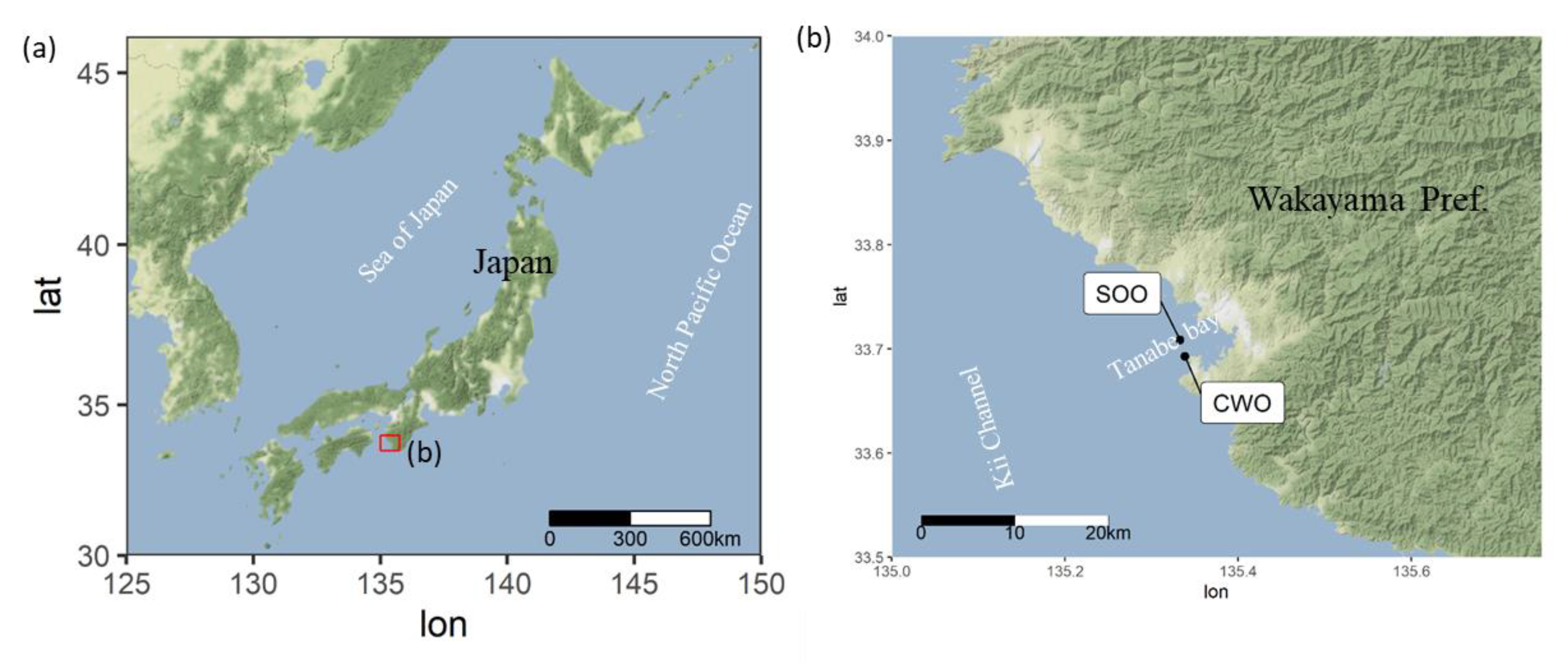
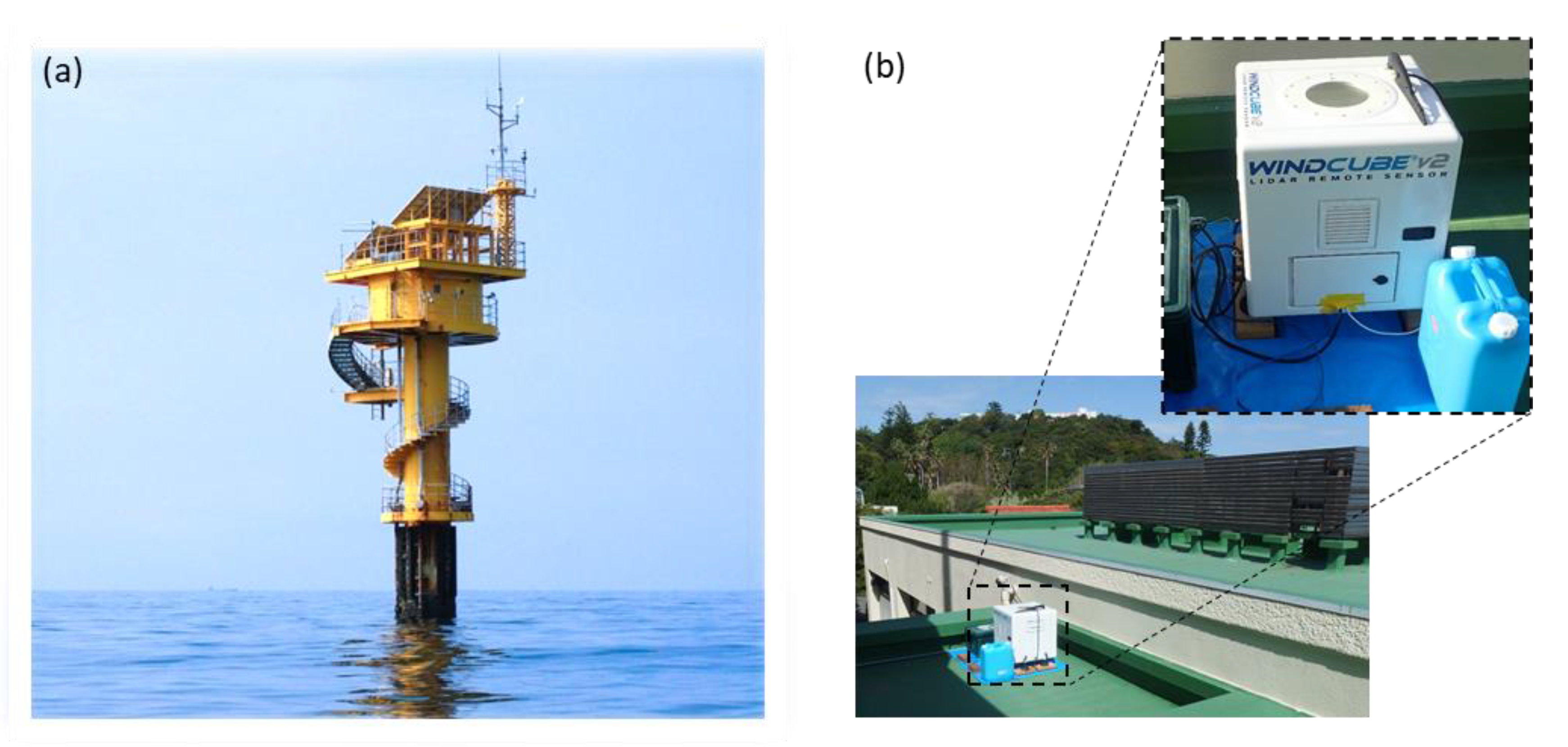
2.1. Observation

The wind measurement sites are located offshore (Shirahama Oceanographic Observatory, SOO) and onshore (Coastal Wind Observation, CWO), located at a distance of approximately 2 km from the offshore site SOO, as presented in Figure 1 and Figure 2. The offshore data collected in this study were obtained from the offshore research platform operated by the Kyoto University Shirahama Oceanographic Observatory in Tanabe Bay) [32]. Analysis was performed using 10 min average wind speed and direction measurements at a height of 23 m at the SOO.

A vertical Doppler LiDAR installed at the CWO (5 m above mean sea level) measured the wind speed and direction at heights ranging from 44 m to 264 m (+4 m was added to the observation height considering the LiDAR was located 4 m above ground level;

Table 1. Summary of the LiDAR observation at SOO.

LiDAR Model	Wind Cube V2
Implementer	LEOSPHERE (Vaisala)
Number of observation heights	12
Observation height *	40, 60, 80, 100, 120, 140, 160, 180, 200, 220, 240, and 260 m
Measuring range	Speed: 0–55 m/s
	Direction: 0–360°
Measuring accuracy	Speed: 0.1 m/s
	Direction: 2°
Averaging time	10 min

* For the analysis height, 4 m was added to the observation height because the LiDAR was located at 4 m above ground level.

). Leosphere WindCube V2 [33], a common reference remote sensor employed for vertical LiDAR measurement by the Doppler beam swinging strategy [34], was used to measure wind speed and direction at the CWO. The accuracy of WindCube V2 has been previously validated [35].

In this study, the wind conditions at the SOO were estimated using the CFD and mesoscale models, and the SOO measurements were used to validate the results. The CWO measurements were used as input data for the CFD model and as validation data for the vertical wind profile estimated at the coastal site.

Figure 3 presents the monthly average wind speeds measured at the offshore (SOO) and onshore (CWO) sites during the study period from 25 April 2017 to 19 July 2017. The measurements plotted in the figure were taken at observation heights of 23 m at the SOO and 44 m and 264 m (lowest and highest) at the CWO. Despite the lower observation height at the SOO, the collected wind speeds were higher than those at the CWO (44 m). This indicated that the offshore wind speed is higher than the coastal wind speed, despite being 2 km offshore. The wind speed was particularly high in June at the CWO (264 m), indicating that different wind conditions prevailed in the upper and lower levels.

As wind speeds exceeding the cut-in wind speed limit are important in wind resource assessment, this study only used the data when wind speed was higher than 2 m/s at 264 m at the CWO. The validation data used in the analysis consisted of 2064 samples, amounting to 65.3% of hourly data. All the figures and tables presented in this study are based on that dataset. The 10 min average wind speed and direction data were used as both the input data and validation data.

2.2. Numerical Simulations

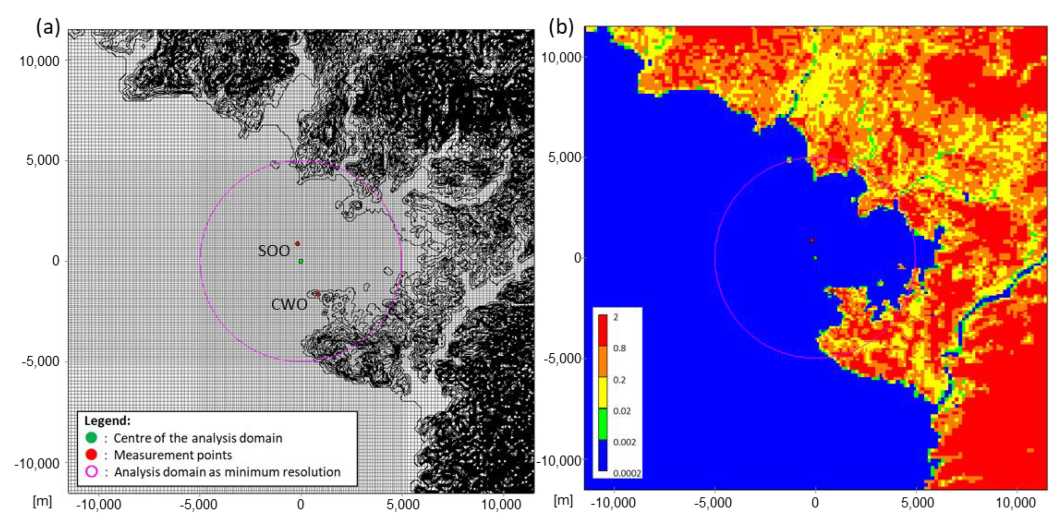
Generally, numerical models used for wind resource assessment may be classified into two types: (1) CFD and (2) mesoscale models. In this study, we used MASCOT [7,8] as a CFD-based non-linear model and WRF [18] as a mesoscale model to estimate wind conditions.

Table 2. Numerical models used in this study.

	CFD Model	Mesoscale Model
Model	MASCOT	WRF
General description	A CFD-based non-linear model developed by Tokyo University, implementing the k-ε model, for the prediction of local wind in complex terrain in Japan.	A mesoscale model developed by the National Center for Atmospheric Research, and others, for atmospheric research and operational forecasting applications.
Wind field calculation	Steady calculation of wind fields for each of the 16 wind directions.	Continuous calculation of wind fields generated by time-varying boundary conditions.
Wind conditions at the target site	Wind conditions at a target site were calculated based on the measured wind conditions at a reference site and simulated wind fields.	Time series of the wind speed and direction at the grid point corresponding to the target site was extracted.
Boundary conditions (upstream)	Steady flow upstream in a virtual region, where the topography is flat and roughness is constant.	Global or regional analysis (re-analysis).

presents the features of these numerical models.

One of the main differences between the CFD and mesoscale models is the input data. In the CFD model (MASCOT), wind measurements at a reference site are used as input data to estimate the surrounding wind conditions, similar to the WAsP model [25]. Meanwhile, in the mesoscale model (WRF), grid point values (GPVs) of global or regional analyses are used for calculation in lieu of measurement data as initial and boundary values. Another difference between the two models is their output parameters: the CFD model yields only wind parameters, such as wind speed and direction, as outputs, whereas the mesoscale model yields meteorological elements, such as temperature, moisture, and atmospheric radiation, in addition to wind parameters.

2.2.1. CFD Model

MASCOT, a non-linear CFD model, is frequently used for onshore wind resource assessment in Japan owing to its good performance in simulating a high-resolution wind field over complex terrain. The CFD model also serves as the technical basis for the certification of onshore and offshore wind power facilities in Japan. In MASCOT, neutral wind conditions are simulated depending on the terrain and roughness length in the calculation domain. Wind calculation using the CFD model is based on the relative wind speed in each direction. It therefore becomes important to correctly estimate both the wind speed rate and wind direction differences.

In this study, wind measurements via LiDAR at the onshore site, CWO, were used as input data in MASCOT to estimate the wind conditions at the offshore site, SOO. The configurations and calculation domain of the CFD model are listed in

Table 3. Configurations of the CFD model.

Model	MASCOT 3.2.4
Center of the calculation domain	N33°42′28.213″, E135°19′44.400″ (Tokyo Datum)
Elevation data	50 m grid DEM data *
Ground roughness	Based on the 100 m mesh land use data *
Size of the calculation domain	23 km × 23 km
Wind direction	16 directions
Minimum horizontal resolution	100 m
Minimum vertical resolution	5 m
Calculation domain as minimum resolution	Within a 5000 m radius
Number of mesh	5,160,672

* Provided by the Geospatial Information Authority of Japan.

and presented in Figure 4, respectively. The 50 m digital elevation model [36] published by the Geographical Survey Institute was used as terrain data, and roughness length information was generated based on the land use data published by the Ministry of Land, Infrastructure, Transport, and Tourism [37] (

Table 4. Roughness length table for various types of land use in the CFD model.

Type	Roughness Length (m)
Rice field (Tanbo)	0.03
Field	0.1
Orchard	0.2
Other wood field	0.1
Forests	0.8
Wasteland	0.03
High buildings	1
Low buildings	0.4
Transportation area	0.1
Other area	0.03
Lakes and ponds	0.0002
River A: Does not include artificial land use in river areas	0.001
River B: Artificial land use in riverbeds	0.001
Beach	0.03
Sea	0.0002

). These methods were the default configurations used in the MASCOT analysis. The distribution of the terrain (Figure 4a) and roughness length (Figure 4b) demonstrate that forest areas in a complex terrain were widespread in the land part of the domain.

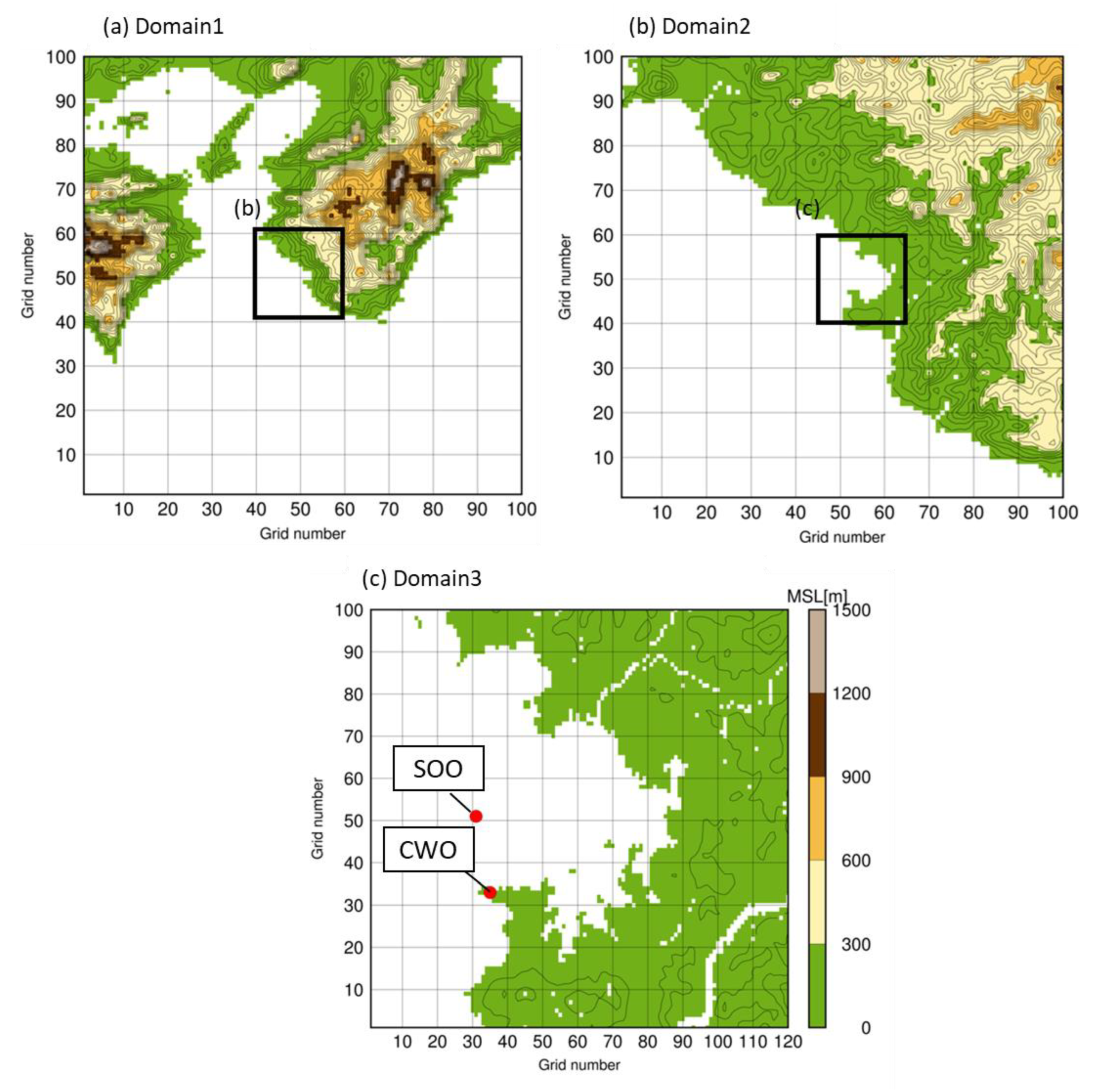
2.2.2. Mesoscale Model

WRF is a mesoscale model, and is frequently used in weather forecasting and wind resource assessment. Unlike the CFD model, the mesoscale model usually does not use in situ data as the input; instead, it uses global or regional analysis data, which express lower-resolution meteorological fields for a broader area as its initial and boundary conditions. This study used the mesoscale model (MSM) GPV data from the Japan Meteorological Agency (JMA) [38] as the input for the meteorological boundary conditions. The configurations for the WRF simulation are almost the same as those used to produce the NEDO offshore wind resource map “NeoWins” [19]; however, the model employs the JMA mesoscale analysis (MANAL) [39] as the input in lieu of MSM-GPV. According to a previous study [40], there were marginal differences in the WRF results obtained between the inputs from the MSM and MANAL, and the accuracy of the mesoscale model in this study may be regarded as the same as that of NeoWins.

Table 5. Configurations of the mesoscale model.

Model	WRF (Advanced Research WRF) ver. 3.8.1
Grids	Domain 1: 2.5 km × 2.5 km, 100 × 100 grids
	Domain 2: 0.5 km × 0.5 km, 100 × 100 grids
	Domain 3: 0.1 km × 0.1 km, 120 × 100 grids
Levels	40 levels (Surface to 100 hPa)
Input data	3-hourly, 0.05° × 0.05° JMA-MSM (for meteorological elements)
	Daily, 0.02° × 0.02° IHSST (for sea surface temperature) [41]
	6-hourly, 1° × 1° NCEP FNL (for soil)
4DDA	Domain 1: Enabled
	Domain 2: Enabled, but excluding below PBL height
	Domain 3: Enabled, but excluding below PBL height
Physics option	Dudhia shortwave scheme
	RRTM longwave scheme
	Ferrier (new Eta) microphysics scheme
	Kain-Fritsch (new Eta) cumulus parameterization scheme
	Mellor-Yamada-Janjic (Eta) TKE PBL scheme
	Monin-Obukhov (Janjic Eta) surface-layer scheme
	Noah land surface scheme

and Figure 5 show the configurations and calculation domains of the mesoscale model used in this study, respectively. The minimum horizontal resolution was configured as a 100 m mesh, similar to the CFD model. Three-stage nesting was implemented by calculation in the mesoscale model (Figure 6). A much wider calculation domain was, therefore, configured in the mesoscale model than in the CFD model.

3. Results and Discussion

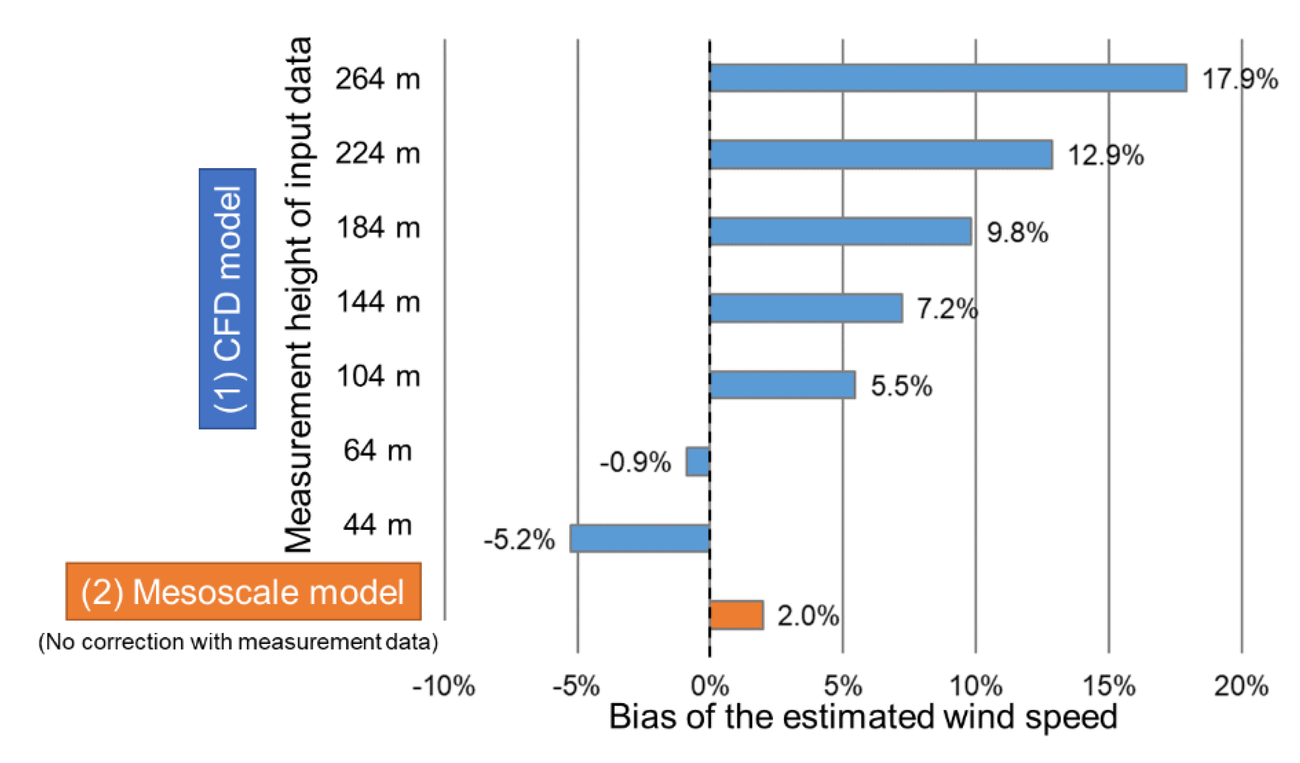
3.1. CFD Model Sensitivity to Observation Height of Input Data

First, we examined the sensitivity of the CFD model to the observation height of the data input. Figure 6 shows the biases of the estimated wind speed at the SOO. The observed average wind speed for the entire analysis period was 4.58 m/s. The bias is expressed as the percentage of this average wind speed hereafter. In the CFD model, the bias was −5.2% when the lowest height LiDAR measurement (44 m) was used as the input. The bias became positive and larger when the upper height measurements were used, reaching +17.9% using data obtained at 264 m. Therefore, the smallest bias (−0.9%) was noted using data at 64 m. However, the mesoscale model had a bias of +2.0%, without any corrections using the LiDAR measurement.

Figure 7 shows the wind speed maps obtained from the CFD model using measurement data at 64 m and 264 m as inputs. Large differences between these maps demonstrate wind speed dependency on the choice of input data. Selecting upper height data as the input led to a higher wind speed field. This is more evidently noted in Figure 8, which presents the vertical profiles of the estimated wind speeds at the SOO obtained by the CFD model, with different input data at the CWO. Based on this, the 23 m height wind speed was found to be the most accurate when the 64 m height data were used. When the upper height data were used as the input, the profile shifted toward a higher wind speed, maintaining a weak vertical shear.

In this study, the offshore target was 23 m in height; however, recently, a typical offshore wind turbine had a hub height of >100 m. This indicates that the CFD model required such an upper height observation as the input because the observation height of the input data should be close to the height of the offshore target. In Japan, it is difficult to build a met mast exceeding 60 m in height due to legal restrictions. Thus, a vertical Doppler LiDAR, with the ability to measure wind speeds up to a few hundred meters above the ground, is an essential observation device to provide input data for the CFD model.

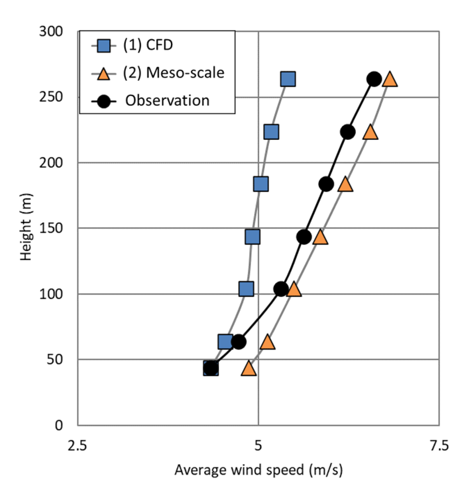
3.2. Vertical Wind Speed Profile at CWO

We compared the vertical wind profiles obtained by the CFD and mesoscale models at the CWO. Figure 9 shows the vertical wind speed profiles estimated with both the models and those observed with the vertical LiDAR. In the CFD model, the 44 m height data were used as the input. The CFD profile exhibited a weaker shear than the observation, underestimating wind speeds at upper heights. Conversely, if wind speeds were normalized based on the upper height wind speed, the lower height wind speed would be higher than the observation owing to the weak shear. This can explain why large positive biases were found at 23 m height at the SOO when using upper height observation data at the CWO as the input for the CFD model (Figure 6).

Alternatively, the mesoscale model had a vertical profile more similar to the observation at the CWO. However, as shown in Figure 9, simulated wind speeds were higher than those observed, especially at lower heights. The relative bias reached +12% at 44 m, but it decreased to +4% at 264 m. Compared with Figure 6, the bias at the SOO (+2.0%) was smaller than the biases at the CWO; however, the observation height at the SOO (23 m) was lower than that at the CWO. This result is the same as that reported for WRF-simulated offshore wind speeds: WRF had a relatively larger positive bias at lower heights in nearshore areas and a smaller bias at offshore sites than at onshore sites [23,24,42].

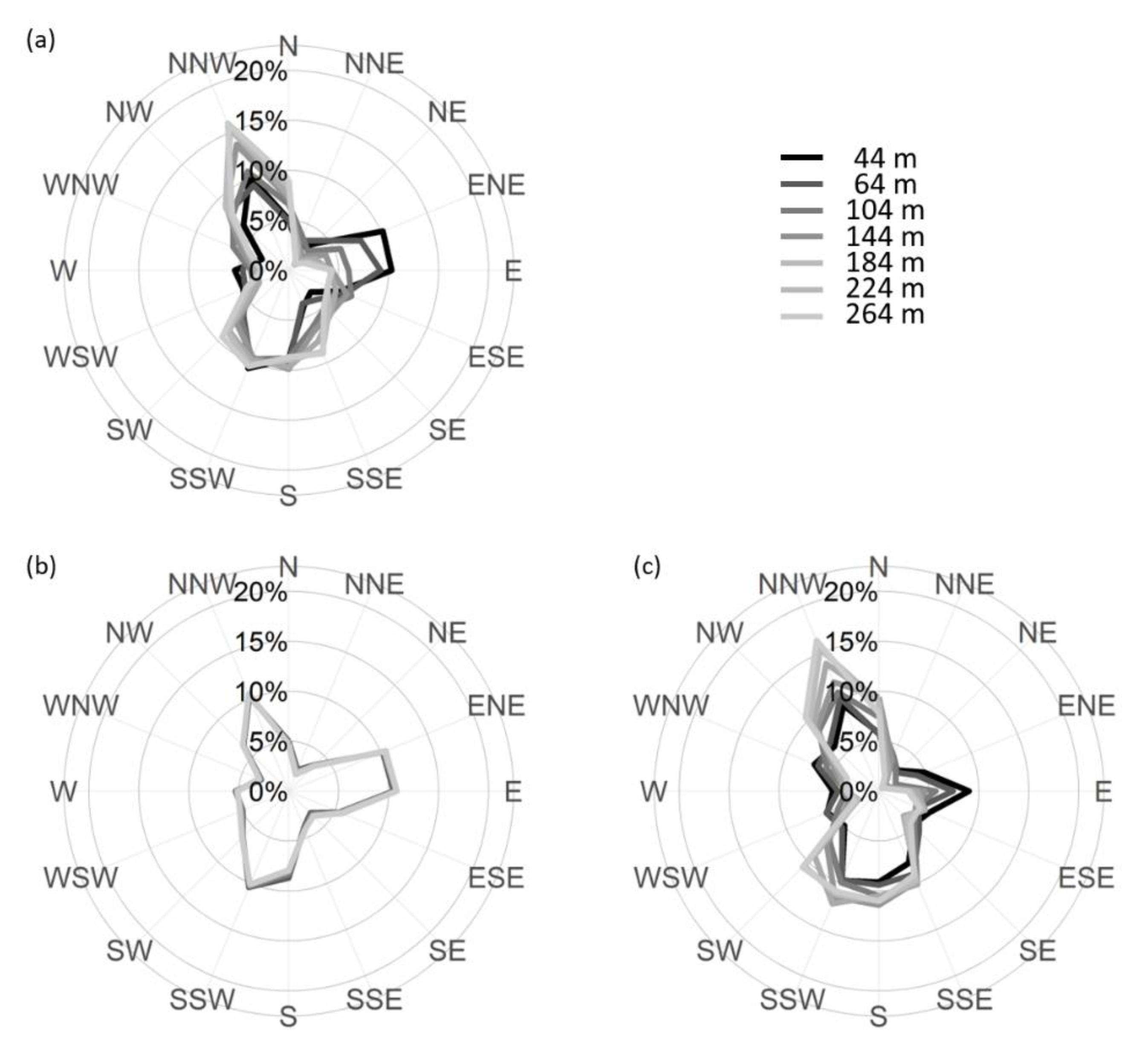
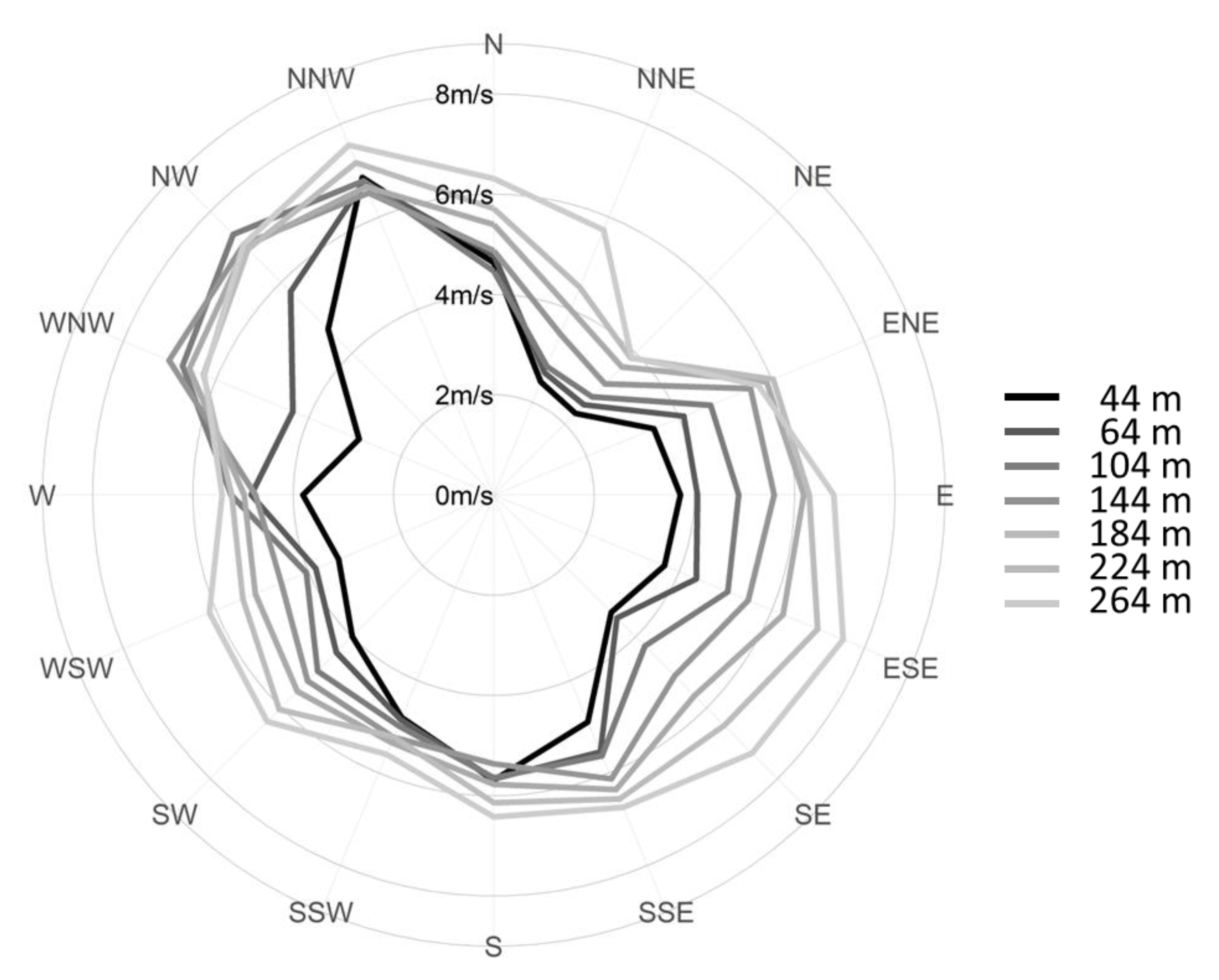
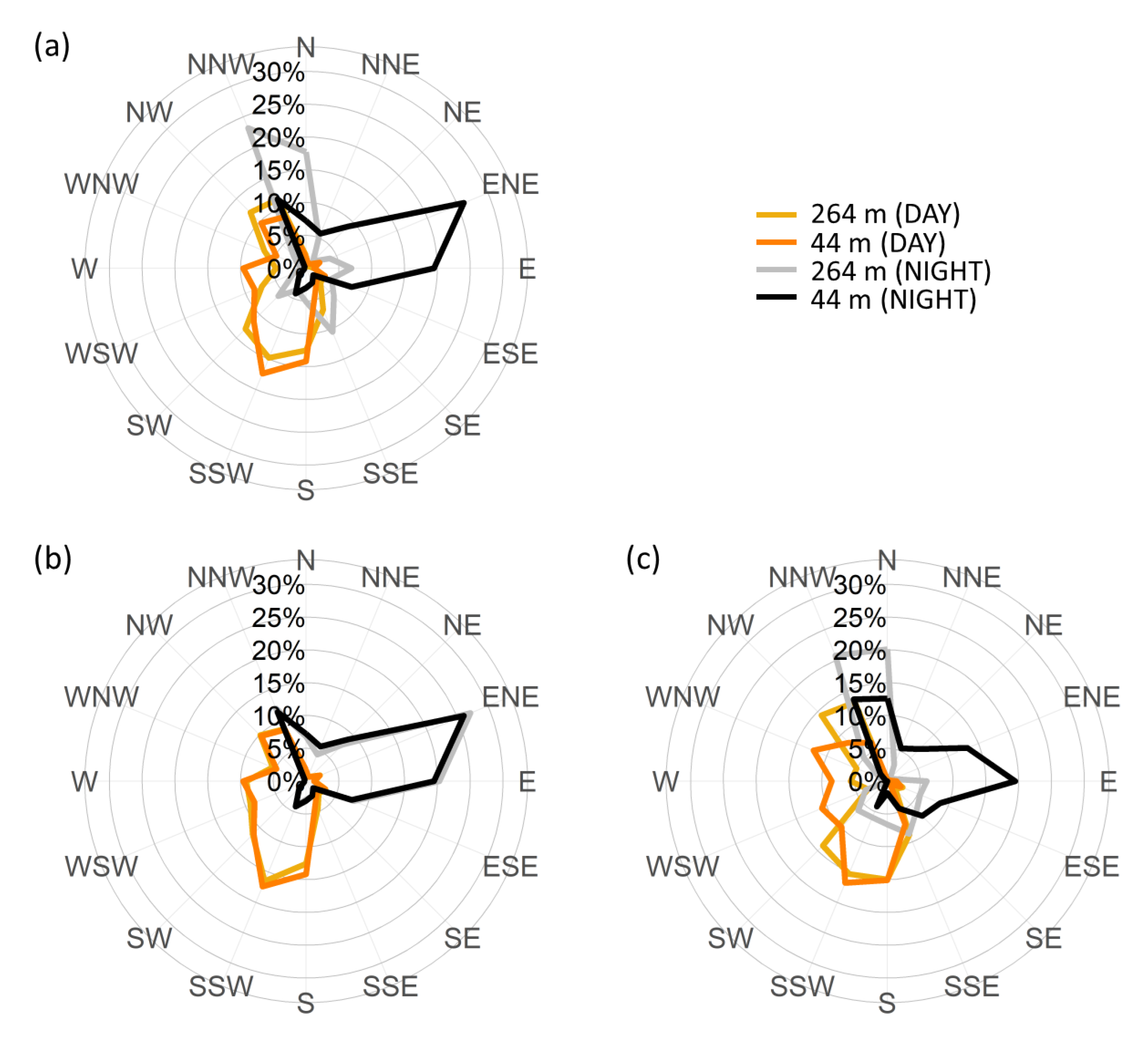
3.3. Features of Wind Direction

As demonstrated in Figure 6, the most accurate estimation from the CFD model could be obtained using the 64 m height measurement as the input data. We were compelled to investigate why 64 m was the most suitable input data height when the CFD model estimated the 23 m height wind speed at the SOO. The answer lies in the wind direction. Figure 10 shows the superimposed wind roses observed at the SOO and CWO. The wind rose at the SOO was similar to that at the 64 m height at the CWO; however, it significantly differed from the wind rose at the 264 m height at the CWO.

Figure 11 shows the wind roses for the observed and estimated winds at the CWO. The wind direction frequencies observed at the CWO differed according to the measurement heights. Easterly winds, which are primarily land breezes during the night, were less frequently measured at the upper heights. This vertical difference in the frequencies of wind direction could be reproduced, to some extent, in the mesoscale model simulation. The wind direction frequencies at all heights were mostly unchanged on the CFD model simulation compared to those of the input data (44 m), because the CFD model accounts for only changes in the wind direction due to dynamical effects.

Figure 12 shows the observed wind speed averaged for each wind direction at the CWO. The average wind speed for each wind direction differed, and the speed of easterly winds was generally weak compared to northern and southern winds. Thus, the use of upper height measurements as input data for the CFD model resulted in a high average wind speed estimation at the SOO because the input data contained a larger frequency of northerly winds, which have a higher wind speed than the easterly ones. Therefore, large positive biases were found at the SOO when upper height observation data at the CWO were used as inputs for the CFD model (Figure 6). In other words, observation data at the CWO with the most similar wind rose to that at the SOO provided the most accurate wind speed estimation at the SOO.

Alternatively, the wind speed patterns from W to NNW differed from other directions, which is attributed to the presence of small hills in these directions at the CWO, which seemed to have the highest effect on the wind at the lowest height of 44 m. Therefore, lower height winds were more affected by topography and the land surface through dynamical and thermodynamical processes than by upper height winds. From this standpoint, upper height observation data were more suitable as input to the CFD model when estimating wind conditions at the hub height of a wind turbine. Therefore, in this study, 64 m (and not 44 m) was the optimal height for the collection of the input data when the CFD model was used to estimate wind speed at 23 m at the SOO.

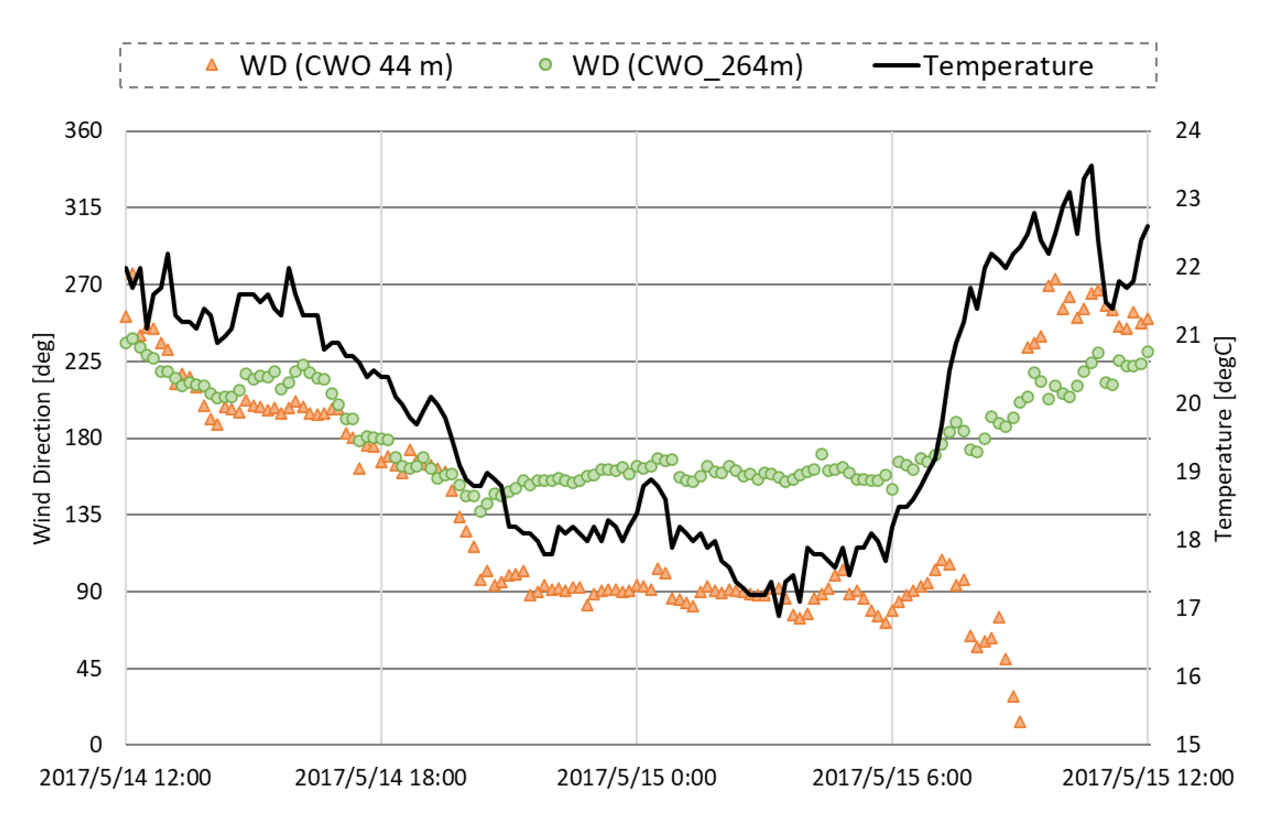
3.4. Wind Condition Formed by Thermodynamic Effects

The wind roses shown in Figure 13 are the same as those in Figure 11, in which the observations at the CWO were plotted and included four wind roses; at two heights (44 m and 264 m) and for two periods (9–18 LT, “daytime” and 0–6 LT, “nighttime”). There were apparent differences in the main wind direction between measurement heights and times. The easterly wind was mostly found at lower heights during nighttime observation (Figure 13a), whereas the southern and northern winds primarily blew at the upper heights. The easterly wind, primarily a land breeze blowing from the land area to the sea at nighttime, was less frequent at the upper heights. This thermodynamic phenomenon is attributed to the thermal difference between the land and sea areas, a phenomenon known as land and sea breeze circulation [43,44].

The Nanki-Shirahama weather observation site, operated by the JMA, is located to the southeast of the CWO at a distance of approximately 4 km. Figure 14 shows a time series of the temperature measurements taken at the site and the wind direction data measured at heights of 44 m and 264 m at the CWO during a typical land breeze period. The easterly land breeze started blowing at 44 m around 20 LT on 14 May, forming a large difference in wind direction between 44 m and 264 at night when the temperature dropped. Thereafter, the land breeze disappeared as the air temperature rose on the morning of 15 May.

Comparing Figure 13a,c, the vertical difference in the wind direction (wind veer) caused by the land breeze could be reproduced to some extent in the mesoscale model simulation. In contrast, in the CFD model simulation, the estimated wind directions at all heights were the same as those at the corresponding heights of the input data (Figure 13b). The wind rose shows this result using input data measured at the lowest height (44 m) at the CWO; the wind rose for 264 m shows the same pattern as that observed at 44 m. Given that the CFD model has been developed as a dynamic model, the vertical change in the wind direction caused by thermodynamic effects cannot be considered. This was probably the main reason for the inferior results obtained for the offshore site using the CFD model, with input data measured at the upper height.

3.5. Wind Speed Map Estimated Using Numerical Models

Figure 15 shows the mean wind speed maps at 23 m, estimated using the two models. In the map of the CFD model (Figure 15a), measurement data collected at 64 m height at the CWO were used as the input. Both maps demonstrate similar wind speed distributions, with lower wind speeds in Tanabe Bay and gradually increasing wind speeds spreading outwards. However, there were apparent differences between the two models in the wind speed gradients from land to sea. A large wind speed gradient was observed near the coastline in the CFD model map, with the weak wind that rapidly transformed into high wind, especially within an approximate 1 km distance from the coastline. In contrast, the wind speed gradients were small in the mesoscale model map (Figure 15b). This characteristic appeared to be similar to the results of previous studies, demonstrating that the WRF model tended to overestimate offshore wind speeds, especially those in the vicinity of the coastlines in Japan [24,45]. Thus, for wind speed distribution, the CFD model map may potentially estimate a more realistic wind speed distribution near the coastline than the mesoscale model map.

4. Conclusions

This study was conducted to investigate the reliability of the CFD and mesoscale models to estimate nearshore wind conditions influenced by the land. This was determined by examining the accuracy and characteristics of offshore wind speeds simulated by the two models. It was therefore determined that if wind conditions are formed by thermal factors, then those numerical models that can thermodynamically reproduce them should be used, such as the mesoscale model. Examinations were performed using in situ measurements from the SOO and a vertical Doppler LiDAR located at the coast (CWO). The main conclusions are summarized below.

• When estimating offshore wind speed based on a CFD model and onshore LiDAR measurements, the estimation accuracy greatly depends on the measurement height of the LiDAR measurements used as input data for the CFD model. In this case, the bias was positive and large when upper height measurements were used as the input. The bias reached +17.9% when the 264 m height data were used. Thus, proper selection of the input height is vital for successful estimation using the CFD model. In general, a height close to the offshore target, such as the hub height of a wind turbine, should be selected as the input data, given that the accuracy of the wind speed shear replicated in a CFD numerical model may be uncertain, as it cannot replicate thermal effects.
• In the study area, LiDAR measurements at the CWO demonstrate that the vertical shear and veer of the wind were not dynamically influenced by thermodynamic phenomena, such as land and sea breezes. The CFD model cannot reproduce wind veer well as it does not consider thermodynamic effects. This is one of the primary causes of the inaccurate estimation by the CFD model for the offshore site.
• Compared to the CFD model, the mesoscale model accurately replicated the wind conditions formed by the thermodynamic effect, exhibiting a bias of +2.0% in the SOO estimation, without any corrections using observation data. Regarding the wind speed profile at the CWO, large estimation errors were, however, found at lower heights compared to upper heights. Additionally, the gradient of the wind speed from land to sea estimated by the mesoscale model demonstrated a smaller gradient, as has been previously reported by studies conducted in Japan [24,45]. These results indicate that the mesoscale model is likely to overestimate wind speed in nearshore waters, especially in areas extremely close (e.g., 1 km) to the coastline.

The main limitation of this study is that only one coastal area was analyzed. To improve the generalizability of the proposed method for nearshore areas, it is necessary to study coastal areas with different wind conditions (e.g., the frequency distribution of land and sea winds) and topography (e.g., the complexity of coastlines and land topography). Although this study was conducted during the warm season when winds are relatively weak, from the perspective of wind power generation, attention should be paid to the cold season, when winds are stronger. The thermal environment during the cold season is expected to be different from that during the warm season, as the sea area is likely to be unstable, whereas the land area is likely to be stable. Therefore, it is necessary to conduct further comparative studies across different seasons.

References

1. Obane, H.; Nagai, Y.; Asano, K. Assessing the potential areas for developing offshore wind energy in Japanese territorial waters considering national zoning and possible social conflicts. Mar. Policy 2021, 129, 104514. [Google Scholar] [CrossRef]
2. JWPA, Offshore Wind Power Development in Japan. 2017. Available online: https://jwpa.jp/cms/wp-content/uploads/20170228_OffshoreWindPower_inJapan_r1.pdf (accessed on 17 October 2022).
3. Dodd, J. Do we still need met masts? Wind. Mon. 2018, 34. Available online: https://www.windpowermonthly.com/article/1458018/need-met-masts (accessed on 17 October 2022).
4. Peña, A.; Hasager, C.; Gryning, S.; Courtney, M.; Antoniou, I.; Mikkelsen, T. Offshore wind profiling using light detection and ranging measurements. Wind Energy 2009, 12, 105–124. [Google Scholar] [CrossRef]
5. Shimada, S.; Takeyama, Y.; Kogaki, T.; Ohsawa, T.; Nakamura, S. Investigation of the fetch effect using onshore and offshore vertical LiDAR devices. Remote Sens. 2018, 10, 1408. [Google Scholar] [CrossRef] [Green Version]
6. Shimada, S.; Kogaki, T.; Takeyama, Y.; Ohsawa, T.; Nakamura, S.; Kawaguchi, K. Accuracy of offshore wind measurements using a scanning LiDAR. Grand Renew. Energy 2018, 35, 135–138. [Google Scholar]
7. MEASNET. MEASNET Evaluation of Site-specific Wind Conditions—Version 3; MEASNET: Madrid, Spain, 2022. [Google Scholar]
8. IEC. IEC61400-12-1 Wind Turbines—Part 12-1: Power Performance Measurements of Electricity Producing Wind Turbines, 3rd ed.; IEC: London, UK, 2022. [Google Scholar]
9. Ishihara, T.; Hibi, K. Numerical study of turbulent wake flow behind a three-dimensional steep hill. Wind. Struct. 2007, 5, 317–328. [Google Scholar] [CrossRef]
10. Ishihara, T.; Yamaguchi, A.; Fujino, A. Nonlinear model for predictions of turbulent flow over steep terrain. In Proceedings of the World Wind Energy Conference and Exhibition, Berlin, Germany, 2–6 July 2002; pp. 1–4. [Google Scholar]
11. Uchida, T.; Ohya, Y. Micro-siting technique for wind turbine generators by using large-eddy simulation. J. Wind Eng. Ind. Aerodyn. 2008, 96, 2121–2138. [Google Scholar] [CrossRef]
12. Sempreviva, A.M.; Barthelmie, R.J.; Pryor, S.C. Review of methodologies for offshore wind resource assessment in European seas. Surv. Geophys. 2008, 29, 471–497. [Google Scholar] [CrossRef]
13. Peña, A.; Hahmann, A.; Hasager, C.; Bingöl, F.; Karagali, I.; Badger, J.; Badger, M.; Clausen, N. South Baltic Wind Atlas. 2011. Available online: http://orbit.dtu.dk/files/5578113/ris-r-1775.pdf (accessed on 17 October 2022).
14. Hahmann, A.N.; Lennard, C.; Badger, J.; Vincent, C.L.; Kelly, M.C.; Volker, P.J.; Argent, B.; Refslund, J. Mesoscale Modeling for the Wind Atlas of South Africa (WASA) Project; E No. 0050; DTU Wind Energy: Roskilde, Denmark, 2014; Volume 80. [Google Scholar]
15. Chang, R.; Zhu, R.; Badger, M.; Hasager, C.B.; Xing, X.; Jiang, Y. Offshore wind resources assessment from multiple satellite data and WRF modeling over South China Sea. Remote Sens. 2015, 7, 467–487. [Google Scholar] [CrossRef] [Green Version]
16. Mattar, C.; Borvarán, D. Offshore wind power simulation by using WRF in the central coast of Chile. Ren. Energy 2016, 94, 22–31. [Google Scholar] [CrossRef]
17. Washio, T.; Sakamoto, N.; Nakashima, S.; Aoki, I.; Kawaguchi, K.; Nagai, T.; Nakai, K. Construction of ocean observation tower system off the Kita-Kyushu city for offshore wind farm design. J. Jpn Soc. Civ. Eng. 2013, 69, I.1–1.6. (In Japanese) [Google Scholar]
18. Skamarock, W.C.; Klemp, J.B.; Dudhia, J.; Gill, D.O.; Barker, D.M.; Wang, W.; Powers, J.G. A Description of the Advanced Research WRF Version 3; Tech. Note TN-475+STR; National Center for Atmospheric Research: Boulder, CO, USA, 2008; pp. 1–96. [Google Scholar]
19. NEDO. The NEDO Offshore Wind Information System. Available online: https://appwdc1.infoc.nedo.go.jp/Nedo_Webgis/top.html (accessed on 17 October 2022).
20. Ohsawa, T.; Kozai, K.; Nakamura, S.; Kawaguchi, K.; Shimada, S.; Takeyama, Y.; Kogaki, T. Accuracy of WRF simulation in the NEDO offshore wind resource map. Proceeding Jpn. Wind. Energy Symp. 2016, 38, 17–20. (In Japanese) [Google Scholar]
21. Ohsawa, T.; Uede, H.; Misaki, T.; Kato, M. Accuracy of WRF Simulations Used for Japanese Offshore Wind Resource Maps. International Conference on Energy and Meteorology. 2017. Available online: http://www.wemcouncil.org/ICEMs/ICEM2017_PRES/ICEM_20170629_1120_Sala_2_Ohsawa.pptx (accessed on 17 October 2022).
22. Shimada, S.; Ohsawa, T.; Chikaoka, S.; Kozai, K. Accuracy of the wind speed profile in the lower PBL as simulated by the WRF model. SOLA 2011, 7, 109–112. [Google Scholar] [CrossRef] [Green Version]
23. Misaki, T.; Ohsawa, T. Evaluation of LFM-GPV and MSM-GPV as input data for wind simulation. J. JWEA 2018, 42, 72–79. [Google Scholar]
24. Kato, M.; Ohsawa, T.; Uede, H.; Shimada, S. Verification of spatial characteristics of WRF-simulated wind speed in Japanese coastal waters. Proc. Jpn. Wind. Energy Symp. 2017, 39, 253–256. (In Japanese) [Google Scholar]
25. Mortensen, N.; Landberg, L.; Troen, I.; Petersen, E. Wind Atlas Analysis and Application Program (WAsP); Risoe-I-666(EN); Getting started; Risø National Laboratory: Roskilde, Denmark, 1993; Volume 1. [Google Scholar]
26. Carvalho, D.; Rocha, A.; SilvaSantos, C.; Pereira, R. Wind resource modelling in complex terrain using different mesoscale–microscale coupling techniques. Appl. Energy 2013, 108, 493–504. [Google Scholar] [CrossRef]
27. Beaucage, P.; Brower, M.C.; Tensen, J. Evaluation of four numerical wind flow models for wind resource mapping. Wind Energy 2014, 17, 197–208. [Google Scholar] [CrossRef]
28. Gasset, N.; Landry, M.; Gagnon, Y. A Comparison of Wind Flow Models for Wind Resource Assessment in Wind Energy Applications. Energies 2012, 5, 4288–4322. [Google Scholar] [CrossRef] [Green Version]
29. Niyomtham, L.; Lertsathittanakorn, C.; Waewsak, J.; Gagnon, Y. Mesoscale/Microscale and CFD Modeling for Wind Resource Assessment: Application to the Andaman Coast of Southern Thailand. Energies 2022, 15, 3025. [Google Scholar] [CrossRef]
30. Jimenez, B.; Durante, F.; Lange, B.; Kreutzer, T.; Tambke, J. Offshore wind resource assessment with WAsP and MM5: Comparative study for the German Bight. Wind Energy 2007, 10, 121–134. [Google Scholar] [CrossRef]
31. Grell, G.; Dudhia, J.; Stauffer, D. A Description of the Fifth-Generation Penn State/NCAR Mesoscale Model (MM5); Technical Report NCAR/TN-398+STR; National Center for Atmospheric Research: Boulder, CO, USA, 1994. [Google Scholar]
32. Kyoto University Shirahama Oceanographic Observatory. Available online: http://rcfcd.dpri.kyoto-u.ac.jp/frs/shirahama/tower_data.html (accessed on 17 October 2022).
33. Windcube Vertical Profiler. Available online: https://www.vaisala.com/en/wind-lidars/wind-energy/windcube (accessed on 17 October 2022).
34. Strauch, R.; Merritt, D.; Moran, K.; Earnshaw, K.; Kamp, D. The Colorado wind-profiling network. J. Atmos. Ocean. Technol. 1984, 1, 37–49. [Google Scholar] [CrossRef]
35. Gottschall, J.; Courtney, M. Verification Test for Three WindCube WLS7 LiDARs at the Høvsøre Test Site; Risø-R-1732(EN); Risø DTU National Laboratory for Sustainable Energy: Roskilde, Denmark, 2010. [Google Scholar]
36. Murakami, H. Accuracy estimation of digital map series data sets published by the Geographical Survey Institute. Geol. Data Process. 1995, 6, 59–64. [Google Scholar] [CrossRef] [Green Version]
37. The Ministry of Land, Infrastructure, Transport and Tourism, Land Use Mesh Data. Available online: http://nlftp.mlit.go.jp/ksj/gml/datalist/KsjTmplt-L03-b.html (accessed on 17 October 2022).
38. JMBSC. MSM-GPV. Available online: http://www.jmbsc.or.jp/jp/online/file/f-online10200.html (accessed on 17 October 2022).
39. JMBSC. MANAL. Available online: http://www.jmbsc.or.jp/jp/offline/cd0380.html (accessed on 17 October 2022).
40. Misaki, T.; Ohsawa, T.; Konagaya, M.; Shimada, S.; Takeyama, Y.; Nakamura, S. Accuracy comparison of coastal wind speeds between WRF simulations using different input datasets in Japan. Energies 2019, 12, 2754. [Google Scholar] [CrossRef] [Green Version]
41. Shimizu, Y.; Ohsawa, T.; Shimada, S. Accuracy validation of offshore wind simulation using WRF with the new SST dataset IHSST. Proc. Jpn. Wind. Energy Symp. 2018, 40, 167–170. (In Japanese) [Google Scholar]
42. Shimada, S.; Ohsawa, T. Accuracy and characteristics of offshore wind speeds simulated by WRF. SOLA 2011, 7, 21–24. [Google Scholar] [CrossRef]
43. Atkinson, B.W. Mesoscale Atmospheric Circulations; Academic Press: Cambridge, MA, USA, 1981; p. 495. [Google Scholar]
44. Simpson, J.E. Sea Breeze and Local Wind; Cambridge University Press: Cambridge, MA, USA, 1994; p. 234. [Google Scholar]
45. Uchiyama, S.; Ohsawa, T.; Araki, R.; Ueda, H.K.; Kouso, K.; Azechi, K. Method for wind resource assessment in nearshore area using WRF-LES and scanning LiDAR. J. JWEA 2019, 43, 70–78. [Google Scholar]
Figure 1. Maps of (a) Japan and (b) the observation sites in the study area.
Resources 11 00100 g001
Figure 2. Wind observation facilities and devices at the (a) Shirahama Oceanographic Observatory (SOO) and (b) Coastal Wind Observation (CWO).
Resources 11 00100 g002
Figure 3. Monthly average wind speeds were measured at the offshore site, Shirahama Oceanographic Observatory (SOO), and onshore site, Coastal Wind Observation (CWO), during the observation period.
Resources 11 00100 g003
Figure 4. (a) Calculation domain and (b) roughness length of the computational fluid dynamic (CFD) model.
Resources 11 00100 g004
Figure 5. Calculation domains of the mesoscale model. (a) Domain 1, (b) Domain 2, and (c) Domain 3, as provided in Table 5.
Resources 11 00100 g005
Figure 6. Bias of the estimated wind speed for the entire analysis period at the Shirahama Oceanographic Observatory (SOO) was obtained using the computational fluid dynamic (CFD) model (with input data from different heights) and the mesoscale model.
Resources 11 00100 g006
Figure 7. Average wind speed map for the entire analysis period at the 23 m height obtained by the computational fluid dynamic (CFD) model. The measurement heights of the input data are (a) 64 m and (b) 264 m.
Resources 11 00100 g007
Figure 8. Estimated vertical wind profiles for the entire analysis period at the offshore site, Shirahama Oceanographic Observatory (SOO). The CFD profiles were calculated using several different height input data at the coastal site, Coastal Wind Observation (CWO; 44–264 m).
Resources 11 00100 g008
Figure 9. Estimated vertical wind speed profile for the entire analysis period at the Coastal Wind Observation (CWO) obtained by the computational fluid dynamic (CFD) model (with input data from the 44 m height) and the mesoscale model.
Resources 11 00100 g009
Figure 10. Wind roses for the LiDAR measurements were obtained at the Shirahama Oceanographic Observatory (SOO; 23 m) and CWO (44 m and 264 m) during the analysis period.
Resources 11 00100 g010
Figure 11. Estimated wind roses at multiple heights at the Coastal Wind Observation (CWO); (a) observation data, (b) computational fluid dynamic (CFD) model (using 44 m height data as the input), and (c) mesoscale model.
Resources 11 00100 g011
Figure 12. Observed wind speed (m/s) averaged for each wind direction for the entire analysis period at the Coastal Wind Observation (CWO).
Resources 11 00100 g012
Figure 13. Wind roses for the entire analysis period at the upper and lower heights at the coastal site, Coastal Wind Observation (CWO). (a) Observations and estimates by (b) the computational fluid dynamic (CFD) model and (c) the mesoscale model using default roughness lengths.
Resources 11 00100 g013
Figure 14. Temporal variations in wind directions (LiDAR at Coastal Wind Observation) and surface air temperature (JWA Nanki-Shirahama station) during a typical land breeze period from 14–15 May 2017.
Resources 11 00100 g014
Figure 15. Average wind speed map for the entire analysis period at 23 m height normalized by observation data at the Shirahama Oceanographic Observatory (SOO). (a) Computational fluid dynamic (CFD) model and (b) mesoscale model. The CFD model used the 64 m height measurement at the Coastal Wind Observation (CWO) as the input.
Resources 11 00100 g015