Different Approaches of Forest Type Classifications for Argentina Based on Functional Forests and Canopy Cover Composition by Tree Species

Abstract

Modern forestry systems rely on typologies of forest types (FTs). In Argentina, several proposals have been developed, but they lack unified criteria. The objective was to compare different approaches, specifically focusing on (i) phenoclusters (functional forests based on vegetation phenology variations and climate variables) and (ii) forest canopy cover composition by tree species. We conducted comparative uni-variate analyses using data from national forest inventories, forest models (biodiversity, carbon, structure), and regional climate. We assessed the performance of phenoclusters in differentiating the variability of native forests (proxy: forest structure), biodiversity (proxy: indicator species), and environmental factors (proxies: soil carbon stock, elevation, climate). Additionally, we proposed a simple FT classification methodology based on species composition, considering the basal area of tree species. Finally, we compared the performance of both proposals. Our findings showed that classifications based on forest canopy cover composition are feasible to implement in regions dominated by mono-specific forests. However, phenoclusters allowed for the increased complexity of categories at the landscape level. Conversely, in regions where multi-specific stands prevailed, classifications based on forest canopy cover composition proved ineffective; however, phenoclusters facilitated a reduction in complexity at the landscape level. These results offer a pathway to harmonize national FT classifications by employing criteria and indicators to achieve sustainable forest management and conservation initiatives.

1. Introduction

Forest management and conservation planning are crucial for maximizing implementation efficiency across territories and contributing to both national and international agreements [1,2,3]. Argentina, in particular, has emerged as a global priority for urgent conservation action due to its rich biodiversity, essential ecosystem services, and decreasing rates of habitat loss [4,5]. While various assessments of global management and conservation priorities exist, such as sustainable forest management practices (e.g., silvopastoral systems) or expanding protected area networks to enhance biodiversity conservation [6,7], developing optimal management and conservation strategies necessitates a deeper understanding of natural ecosystems [8,9,10]. To design effective forest management and conservation strategies, specific tools based on ecological and functional characteristics are essential. Mapping forest tree species and forest types (FTs) plays a crucial role in habitat and biodiversity assessment, as well as in proposing specific management strategies for natural forest resources [9,11,12,13,14,15]. However, mapping FT for large areas (e.g., the country level) using ground-based data is often logistically challenging [12,16], being more frequent in temperate cold forests with simple and predictable stand structures than complex rainforests in the tropics [17,18].

Argentina promulgated National Law 26,331/07, known as “Minimum Budgets for Environmental Protection of the Native Forests”, which includes forest management proposals aimed at social awareness, changes in forest covers, administrative restrictions on forest removal, and long-term forest policies considering resilient socio-economic proposals [1]. Many tools were developed to improve the management and conservation of native forests, e.g., land cover [19,20], forest structure variables [21], potential biodiversity indices [22], soil carbon stocks [23], hotspots of biodiversity conservation concern [24], or human footprint modeling [7]. The National Government of Argentina has proposed seven administrative regions for the nearly 40 million hectares of native forests [25,26], facilitating regional policies and the implementation of goals outlined in National Law 26,331/07 across the territory [6,27]. However, various institutions have implemented their own criteria for forest management, leading to differences in implementation approaches, e.g., National Parks Administration [27,28,29]. Furthermore, Argentina has signed international agreements such as the Kyoto Protocol and the Paris Agreement, implementing the “National Plan for Adaptation and Mitigation to Climate Change”, with key targets focused on native forests using initiatives like REDD+ (Reducing Emissions from Deforestation and Forest Degradation). They propose actions that include reducing deforestation and degradation and promoting sustainable management. In this framework, national and provincial governments need accurate information to develop specific policies.

Current global forest maps (e.g., [30,31]) provide valuable information without considering differences in FT. Nonetheless, they still contribute to various conservation efforts [32,33,34]. In Argentina, mapping natural ecosystems (e.g., forest and non-forest areas) has been ongoing for the past 50 years, initially based on floristic and physiographic characteristics (e.g., [35,36,37,38]). Recent advancements in remote sensing and landscape modeling have enhanced these initial efforts. For instance, Morello et al. [29] categorized Argentina into 115 distinct units, integrating social and biophysical perspectives. Oyarzabal et al. [39] further refined this by proposing phyto-geographic units in digital format. Derguy et al. [40] introduced a novel approach based on Holdridge life zones, incorporating climate and soil characteristics. More recently, Silveira et al. [14] introduced a ground-breaking perspective by incorporating vegetation phenology variations (e.g., event timing and greenness) within FT and species or climate variation (hereafter named phenoclusters) to classify native forests using remote sensing. Phenoclusters require a combination of land surface phenology (both vegetation phenological events and greenness measures) and climate variables to characterize functional rather than structural or compositional characteristics of ecosystems while considering the geographical distributions of species [14]. The advantage of using phenoclusters to characterize native forests is that they capture phenology and climate gradients among and within FTs and/or tree species in places with no field data. The cyclic and seasonal greenness information provided by phenoclusters is useful for management efforts for biodiversity, particularly to inform strategic location planning, and can be useful for places where forest ecological information is limited and conservation needs are high, such as in many developing countries [14]. This product was developed for the native forests of Argentina, dividing them into 54 categories across the different forest regions in high-resolution maps (30 m pixel).

Zoning serves as a vital tool for the Argentinian Government to regulate human activities in native forests, where provinces are required to define land use zones, which are updated every five years. However, the lack of precise tools for classifying forests across landscapes poses a significant challenge. There are considerable differences in the interpretation of the “forest” concept across various administrative processes in Argentina (see [41]). Consequently, ensuring the effectiveness of sustainable forest policies remains a primary challenge for governments, necessitating the exploration of new alternatives to bridge this knowledge gap. Presently, existing classifications operate at large scales, often resulting in the inadequate representation of many ecosystems within national forest regions [6]. Modern rational forestry systems rely on forest typologies [42] for their implementation. One traditional approach involves classifying forest ecosystems into FTs characterized by distinctive attributes and composed of specific sets of tree species within a particular area [43], where each country may adapt this system to suit its unique circumstances and needs [44]. For this, many alternatives can be implemented by including taxonomy, assemblage of species, phenology, growth and development phases, soil, topography, etc. (e.g., [45,46,47,48]). While many classifications are theoretically grounded, few explore practical implementation issues allowing for the feasibility of implementation in the field. Huertas Herrera et al. [49], for example, proposed an alternative FT classification in Southern Chile based on the contribution of the basal area (BA) of each species in the stand. This approach utilizes forest inventory data and can be readily replicated by technicians or researchers.

Currently, various FT classifications are in use for zoning and planning native forests at national or regional scales in Argentina. However, these classifications lack unified criteria across different levels and are often based on limited field data (e.g., legends used by MAyDS during the implementation of different initiatives) [25,26]. Many of these classifications highlight the underrepresentation of certain FT classes in the landscape or include dominant species with little effective representation within the native forests. In this context, there is a need to develop a unified methodological proposal for determining, classifying, and characterizing the different FTs of native forests in Argentina. This proposal should be based on easily measurable metrics obtained during forest inventories at different scales. The objective was to compare two different approaches to FT classification in Argentina based on (i) functional forests (phenoclusters) and (ii) forest canopy cover composition by tree species. The aim was to create country-level FT classifications that emphasize the role of native forests in different regions, ranging from temperate forests to rainforests. These classifications should be valuable for decision-making, management and conservation policies, and scientific research and should be flexible enough to accommodate updates, considering the potential impact of climate change and human modifications on the original characteristics or distributions of tree species. The specific objectives were to (i) determine the performance of phenoclusters to differentiate the variability of native forest characteristics (proxy: forest structure), potential biodiversity (proxy: potential habitat of indicator species), and environment where they grow (proxies: soil carbon stock, elevation, regional climate); (ii) determine the performance of phenoclusters to capture different ecological relationships among the studied variables; (iii) propose a simple classification methodology based on forest canopy cover composition by tree species; and, finally, (iv) compare both approaches of FT classifications and discuss the feasibility of implementation across Argentina. By addressing these objectives, we aimed to develop a robust and comprehensive FT classification system that enhances our understanding of native forests in Argentina and supports informed decision-making and conservation efforts.

2. Materials and Methods

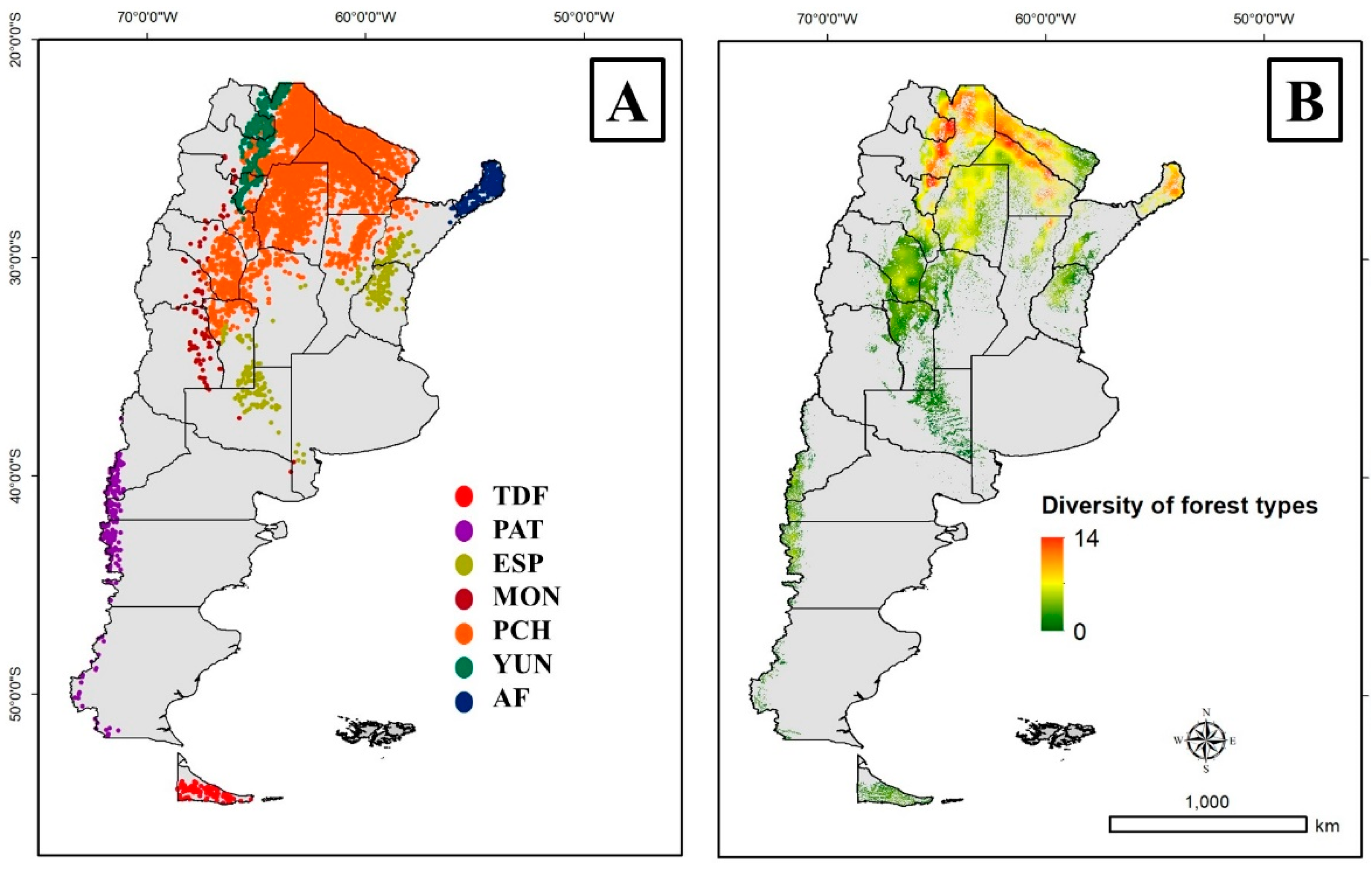
2.1. Study Area

The study area was the native forests of Argentina, distributed between 20° and 60° SL and between 50° and 80° WL across 24 administrative provinces. The National Government of Argentina has divided the native forests into distinct administrative regions [6], including (Figure 1A) (i) Andean–Patagonian forests composed of insular forests of Tierra del Fuego (TDF) and continental forests along the Andes Mountains (PAT); (ii) Delta and the islands of Paraná river (DEL), which occupy a narrow strip of forests from north to south in NE Argentina; (iii) Espinal forests (ESP); (iv) Monte forests (MON); (v) Parque Chaqueño forests (PCH); (vi) Yunga rainforests (YUN); and (vii) Atlantic forests (AF) [25,26]. We used a mask of native forest cover for further analyses, as proposed by Silveira et al. [14], which included areas with trees taller than 5 m in height and with 10% canopy cover using the Global Forest Change dataset [30].

2.2. Forest Type Classification Based on Phenoclusters

The first FT classification proposal used the functional forest categories (phenoclusters) proposed by Silveira et al. [14] based on land surface phenology, climate patterns, the normalized difference vegetation index (NDVI), and other related indexes, and is available in a GRID of 30 m spatial resolution. This layer included 54 categories, divided by forest regions as described before. To test the performance of the phenoclusters as potential FT classifications, we used different available products for the forest regions across Argentina, including the following. (i) The potential biodiversity index (RICH) developed by Martinuzzi et al. [22] for the different forest regions, except the Monte forests, where few available native forest data exist. A layer presented one index (0–100) based on the potential habitat of indicator species by forest region (n = 80 high-profile species of trees, birds, and mammals associated with native forests and representative of each specific forest region) and is available in a GRID of 1 km spatial resolution. (ii) Soil organic carbon stock (SOC, ton·ha⁻¹ in the first 30 cm soil layer) developed by Peri et al. [23] for the different forest regions, which is available in a GRID of 200 m spatial resolution. (iii) Forest structure variables modeled by Silveira et al. [21], including BA (m²·ha⁻¹), crown cover (CC, %), dominant tree height (DH, m), and total over bark volume (TOBV, m³·ha⁻¹) for the different forest regions, which are available in GRIDs of 30 m spatial resolution. (iv) Elevation (ELE, m.a.s.l.) was derived from the SRTM (shuttle radar topography mission) [50], which is available in GRIDs of 30 m spatial resolution. (iv) Climate variables, where we extracted the annual mean temperature (AMT, °C), iso-thermality (ISO), and annual precipitation (AP, mm·yr⁻¹) from WorldClim 2 [51], available in GRIDs of 1 km spatial resolution.

For data extraction of these layers, we employed the hexagonal binning technique, a spatial methodology that offers the advantage of integrating different pixels (e.g., averaging values for each pixel) within polygonal regions to effectively capture spatial patterns [52]. We implemented a hexagonal binning process that involved one spatial matrix dividing the territory of Argentina into hexagonal areas of 5000 ha each [13,53]. We excluded hexagons that presented less than 10% of native forest cover (e.g., <500 ha at each hexagon). Then, we obtained the mean data values for the different studied variables, and the most frequent phenocluster category at each hexagon was selected for further analyses.

2.3. Forest Type Classification Based on Forest Canopy Cover Composition by Tree Species

For the second FT classification proposal, we used forest canopy cover composition by tree species as the main variable to construct a classification. We obtained the forest structure information and tree species assemblages from 3788 field plots (Figure 1A), corresponding to the Second National Forest Inventory (NFI2, 2015–2020) collected by the National Government of Argentina [54]. Detailed information on NFI2 is at SGAyDS [26]. This inventory was carried out on a systematic grid of 10 km × 10 km, measuring all trees classified at the species level. From this, we calculated the total basal area (BA, m²·ha⁻¹), tree density (DEN, n·ha⁻¹), dominant tree height (DH, m), mean tree height (MH, m), and tree regeneration (REG, n·ha⁻¹). Elevation (ELE) and regional climate variables (AMT, AP) were also extracted to characterize these plots (see [13]).

For this second FT classification proposal, each categorization was defined as the contribution of different tree species to the total BA in each plot, regardless of the tree dominance. Firstly, we determined the tree canopy composition, defining a minimum threshold (70% of BA) to analyze each plot, following Huertas Herrera et al. [49]: (i) the stands were considered as mono-specific (MONO) when at least 70% of BA was achieved by a single tree species, (ii) bi-specific (BI) when two tree species were necessary to achieve at least 70% of BA, and (iii) multi-specific (MULTI) when more than two tree species were necessary to reach at least 70% of BA.

The FT classification proposal based on forest canopy cover composition by tree species included three levels. (i) The most general level (Level 1, FT-1) classified the forest typologies using only the name of the most dominant and representative tree genus or the name of the most frequent botanical family involved in plots (e.g., Prosopis + others, Myrtaceae + others). (ii) The intermediate level increased the number of categories (Level 2, FT-2) and considered the scientific name of the most abundant tree species in the BA contribution or, in some cases, we used the most frequent botanical family (e.g., Prosopis alba + others, Euphorbiaceae + others). (iii) Finally, the more detailed classification (Level 3, FT-3) considered the scientific names of the most important tree species (e.g., Prosopis alba, Prosopis nigra + Vachellia caven + Geoffroea decorticans). These levels increased in a number of categories and complexity for different purposes, e.g., as a tool for policymakers in the proposal design of forest management and conservation at the regional scale (FT-1), planning at the regional or local scale (FT-2), or more specific uses, as for technical–scientific studies (FT-3).

Native tree species were classified according to their respective taxonomic divisions and botanical families following the Catalogue of Vascular Plants of the Southern Cone [55]. Exotic tree species (e.g., Ligustrum lucidum) or species without taxonomic determination within the database were not considered in the calculations. However, none of these particular cases was detected as dominant trees in any of the analyzed plots.

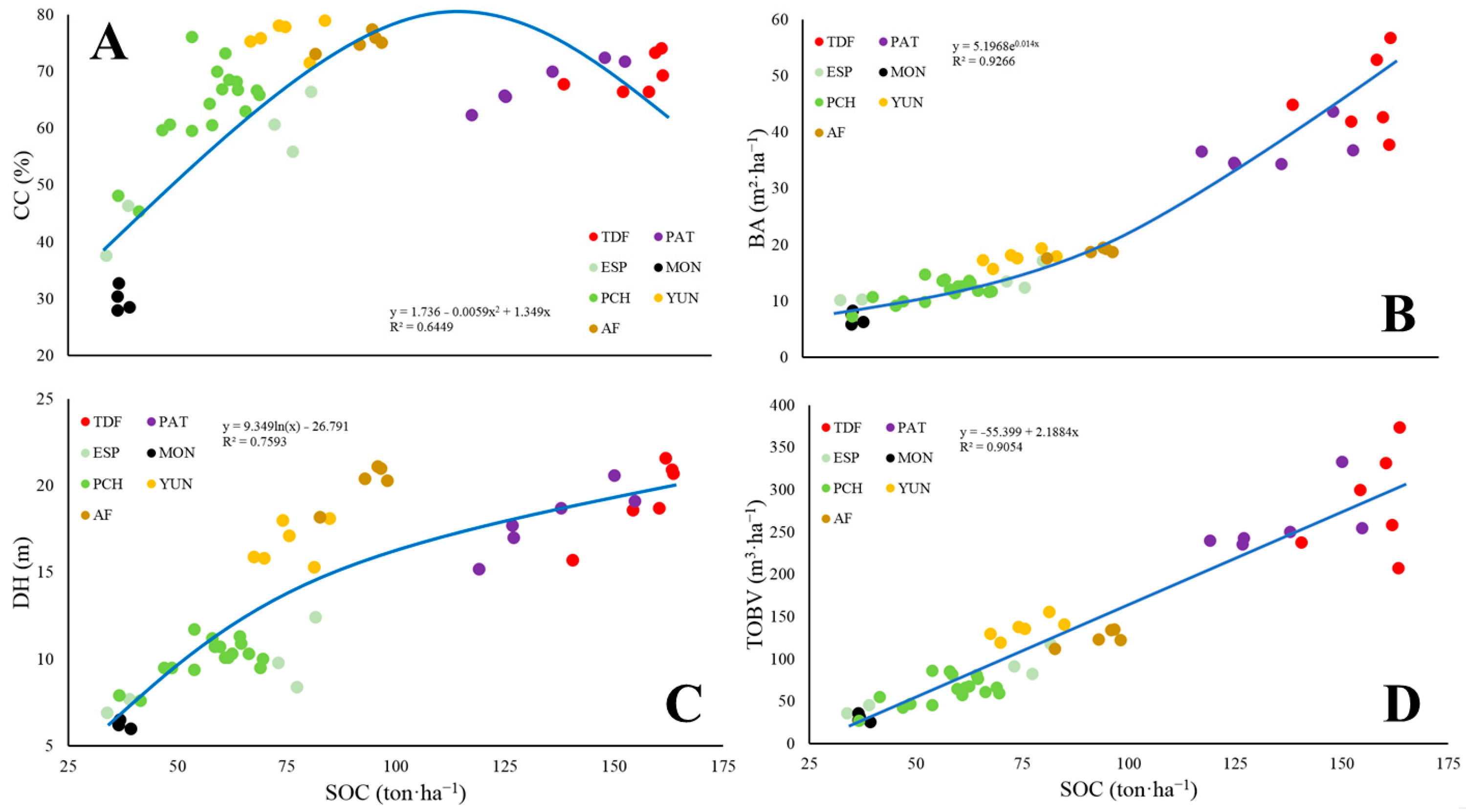
2.4. Statistical Analyses

One-way analysis of variance (ANOVA) was conducted to determine the performance of the FT classification based on phenoclusters in order to differentiate the variability of native forest characteristics by forest regions (TDF, PAT ESP, MON, PCH, YUN, AF), comparing potential biodiversity index (RICH), soil organic carbon stock (SOC), forest structure (BA, CC, DH, TOBV), elevation (ELE), and regional climate (AMT, ISO, AP). FT classification based on phenoclusters was also graphically compared at the country level according to elevation (ELE) and regional climate variables (AMT, ISO, AP) to identify the gradients of the different categories for each forest region. FT classification based on phenoclusters was compared across gradients of SOC and forest structure variables (BA, CC, DH, TOBV), identifying relationships among them and the performance of phenoclusters categories. These relationships were described through linear models and their r²-adj.

FT classification based on forest canopy cover composition by tree species was categorized using the NFI2 plots (n = 3741) in the seven forest regions (TDF, PAT, ESP, MON, PCH, YUN, AF). We quantified how many categories of FT existed for the three defined levels (FT-1, FT-2, FT-3) and their canopy composition (MONO, BI, MULTI) for the entire country and by forest regions, including the categories of FT classification based on phenoclusters. These analyses were mapped into a geographical information system (GIS) for each forest region. The means and standard deviations (SDs) for Level 1 (FT-1) were graphically compared for the different forest regions (AMT vs. AP). Finally, we graphically determined the diversity of FT based on forest canopy cover composition by tree species at the landscape level, using Level 1 (FT-1) of the proposed classification based on forest canopy cover composition by tree species. For this, we applied a 33 × 33 pixel moving window within a 50 km × 50 km grid based on NFI2 plots (n = 3741) into the GIS. Through this analysis, we could assign a number of different FTs at each window by referring to its central pixel. We chose this moving window size because it accommodated an area large enough to encompass animals’ territories while capturing relatively fine-resolution landscape features [14,56]. To obtain the final map, we crossed this analysis with the forest cover mask described before. The resulting map varied between values from 0 to 14, where the diversity of FT was expressed for each pixel in a surrounding area of 50 km × 50 km, allowing us to determine the diversity of FT at the landscape level.

3. Results

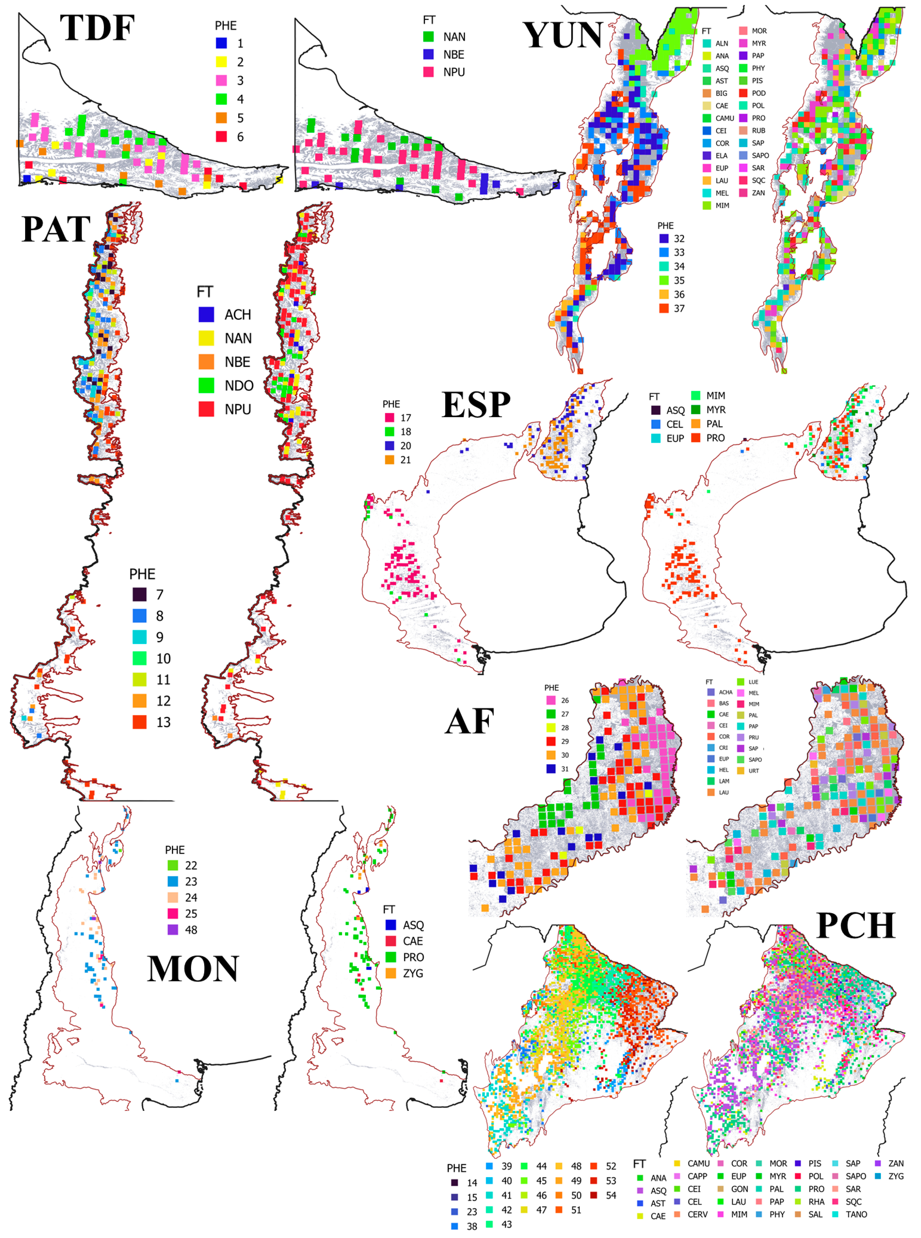
3.1. Forest Type Classification Based on Phenoclusters

The number of phenocluster categories (n = 54) obtained during modeling changed across the different forest regions of Argentina, e.g., TDF (n = 6), PAT (n = 7), DEL (n = 3), ESP (n = 5), MON (n = 4), PCH (n = 17), YUN (n = 6), and AF (n = 6). Some of these phenocluster categories were not analyzed in our study due to their limited occurrence in the landscape, e.g., phenocluster categories of the DEL region, one category at PAT, and one category at AF, which did not include plots of NFI2 (Figure 2). The FT classification of phenoclusters presented significant differences for all the studied variables in the studied forest regions, except in MON for mean annual temperature (AMT) (

Table 1. Analyses of variance comparing phenocluster categories (PHE) at each forest region (TDF = Tierra del Fuego forests, PAT = continental forests along the Andes Mountains, ESP = Espinal forests, MON = Monte forests, PCH = Parque Chaqueño forests, YUN = Yunga rainforests, AF = Atlantic forests). We analyzed potential biodiversity index (RICH), soil organic carbon stock (SOC, ton·ha⁻¹ 30 cm), basal area (BA, m²·ha⁻¹), crown cover (CC, %), dominant tree height (DH, m), total over bark volume (TOBV, m³·ha⁻¹), elevation (ELE, m.a.s.l.), annual mean temperature (AMT, °C), iso-thermality (ISO), and annual precipitation (AP, mm·yr⁻¹).

REGION	PHE	RICH	SOC	BA	CC	DH	TOBV	ELE	AMT	ISO	AP
TDF	1	80.2 bc	154.4 b	41.9 ab	66.4 a	18.6 b	299.7 ab	421.2 d	3.5 a	51.6 c	655.6 e
	2	61.4 a	163.3 b	37.8 a	74.1 c	20.9 c	207.5 a	217.0 bc	4.3 bc	51.2 c	506.5 c
	3	88.1 c	163.6 b	56.7 d	69.3 ab	20.7 c	373.9 b	203.9 b	4.6 c	49.9 b	448.1 b
	4	90.1 c	140.5 a	44.9 b	67.7 a	15.7 a	238.1 a	107.2 a	5.1 d	48.6 a	385.6 a
	5	70.1 b	160.3 b	52.9 cd	66.4 a	18.7 b	331.5 b	382.9 d	3.7 a	51.0 c	533.6 d
	6	57.5 a	161.9 b	42.6 ab	73.3 bc	21.6 c	258.7 a	289.7 d	4.1 ab	51.1 c	521.7 cd
	F (p)	77.54 (<0.001)	51.45 (<0.001)	22.66 (<0.001)	9.64 (<0.001)	34.56 (<0.001)	26.02 (<0.001)	36.20 (<0.001)	41.66 (<0.001)	132.00 (<0.001)	345.81 (<0.001)
PAT	7	62.4 b	137.9 c	34.3 a	70.0 c	18.7 bc	250.4 a	1062.5 a	7.0 c	52.4 c	1046.7 d
	8	66.6 b	154.8 e	36.8 a	71.7 c	19.1 c	254.9 a	1013.4 a	6.8 c	51.0 b	1167.5 e
	9	66.3 b	150.1 d	43.6 b	72.4 c	20.6 d	333.2 b	1123.2 a	6.1 b	51.4 b	1273.9 f
	11	48.3 a	127.0 b	34.2 a	65.5 b	17.0 b	243.2 a	1385.1 b	5.8 ab	52.4 c	785.0 b
	12	49.1 a	126.7 b	34.6 a	65.8 b	17.7 b	235.7 a	1355.2 b	6.1 b	52.5 c	899.0 c
	13	49.5 a	119.1 a	36.6 a	62.3 a	15.2 a	240.0 a	1078.9 a	5.5 a	49.3 a	588.9 a
	F (p)	31.41 (<0.001)	183.20 (<0.001)	11.08 (<0.001)	67.19 (<0.001)	64.57 (<0.001)	17.23 (<0.001)	35.62 (<0.001)	24.53 (<0.001)	61.28 (<0.001)	932.19 (<0.001)
ESP	17	19.5 b	39.0 b	10.3 a	46.4 b	7.7 b	45.9 b	315.0 d	15.9 b	48.6 c	576.3 b
	18	3.2 a	33.9 a	10.2 a	37.6 a	6.9 a	35.8 a	155.2 c	15.1 a	47.5 a	445.3 a
	19	39.0 cd	81.6 d	17.2 d	66.4 e	12.4 e	118.1 e	47.7 a	18.7 c	47.9 ab	1226.0 d
	20	36.2 c	73.1 c	13.5 c	60.7 d	9.8 d	91.6 d	80.4 b	18.8 c	48.0 b	1068.8 c
	21	39.2 d	77.3 d	12.4 b	55.9 c	8.4 c	82.5 c	58.5 a	18.9 d	47.5 a	1064.1 c
	F (p)	733.59 (<0.001)	5368.24 (<0.001)	182.12 (<0.001)	1118.24 (<0.001)	468.36 (<0.001)	1323.15 (<0.001)	824.95 (<0.001)	4599.80 (<0.001)	196.28 (<0.001)	6567.81 (<0.001)
MON	22	--	36.5 a	5.9 a	27.9 a	6.2 ab	28.0 ab	185.1 a	15.5	48.4 a	292.9 b
	23	--	39.4 b	6.3 a	28.5 a	6.0 a	25.6 a	448.5 b	15.4	48.3 a	289.9 b
	24	--	36.6 a	7.6 bc	30.4 b	6.3 b	35.8 c	1461.7 c	15.6	50.4 b	194.6 a
	25	--	36.8 a	8.3 c	32.7 b	6.5 b	31.9 bc	202.1 a	15.6	48.1 a	361.4 c
	F (p)	--	7.99 (<0.001)	18.49 (<0.001)	6.70 (<0.001)	8.58 (<0.001)	38.13 (<0.001)	196.66 (<0.001)	0.98 (0.400)	40.17 (<0.001)	207.66 (<0.001)
PCH	38	30.6 f	58.6 f	13.8 i	60.5 c	10.7 f	81.9 jk	858.3 f	17.5 b	50.1 cd	596.2 b
	39	30.1 f	69.0 k	11.6 ef	66.6 e	9.5 bc	66.1 fgh	71.4 a	19.9 d	49.8 c	987.2 j
	40	35.3 g	58.0 f	13.6 hi	64.3 d	11.2 gh	85.5 k	638.7 e	19.4 c	51.7 gh	642.4 de
	41	18.3 b	41.5 b	10.7 d	45.4 a	7.6 a	55.5 d	925.3 g	16.8 a	49.3 b	527.7 a
	42	56.2 j	61.6 h	12.6 g	73.2 i	10.1 d	66.1 gh	131.7 b	22.4 k	54.3 j	847.7 i
	43	29.9 f	60.9 gh	11.4 e	66.9 ef	10.1 d	57.5 de	155.0 b	21.4 fg	51.3 fg	801.7 h
	44	42.4 h	59.8 fg	12.0 f	70.0 h	10.7 ef	64.8 fg	215.1 c	22.1 i	52.5 i	766.2 g
	45	23.9 d	48.7 d	10.0 c	60.7 c	9.5 b	47.1 c	305.9 d	20.6 e	50.2 cd	621.5 cd
	46	34.9 fg	69.6 k	11.7 ef	65.9 de	10.0 cd	59.5 de	280.5 bcd	22.3 jk	51.5 fgh	791.7 gh
	47	20.8 c	53.8 e	9.8 c	59.6 c	9.4 b	45.8 c	232.9 cd	20.5 e	50.3 d	662.9 e
	48	26.5 e	47.0 c	9.2 b	59.7 c	9.5 b	42.4 b	253.4 d	21.4 fg	50.7 e	609.7 bc
	49	5.6 a	36.7 a	7.3 a	48.1 b	7.9 a	26.9 a	223.0 cd	20.4 e	48.0 a	530.4 a
	50	39.1 g	62.5 hi	12.6 g	68.5 fg	10.3 d	68.1 h	334.7 d	21.8 hi	51.9 h	708.3 f
	51	49.1 i	64.3 ij	13.6 i	68.2 g	11.3 h	81.0 j	78.4 a	21.7 gh	51.5 g	1126.7 k
	52	39.3 gh	53.8 e	14.7 j	76.1 j	11.7 h	86.1 jk	256.3 bcd	22.3 hij	53.1 i	652.3 cde
	53	38.1 g	64.6 j	13.3 h	66.7 e	10.9 fg	76.9 i	77.1 a	21.5 fgh	51.4 fg	1160.3 l
	54	29.8 ef	66.4 jk	11.8 ef	63.0 d	10.3 de	61.0 ef	112.9 ab	20.4 e	50.9 ef	1017.8 j
	F (p)	460.20 (<0.001)	784.09 (<0.001)	588.23 (<0.001)	725.22 (<0.001)	369.69 (<0.001)	739.89 (<0.001)	1044.68 (<0.001)	963.78 (<0.001)	331.25 (<0.001)	2617.41 (<0.001)
YUN	32	65.9 e	84.9 e	17.9 c	78.9 d	18.1 c	140.8 c	1187.5 c	17.6 c	53.3 b	729.3 c
	33	54.2 c	69.9 ab	15.7 a	75.8 bc	15.8 a	119.3 a	765.2 b	19.5 d	52.0 a	742.5 c
	34	73.5 e	74.2 bc	18.1 c	78.1 d	18.0 c	137.8 c	616.8 a	20.8 e	51.5 a	861.7 d
	35	60.4 d	75.6 c	17.6 bc	77.8 d	17.1 b	136.1 c	620.4 a	21.1 e	51.5 a	987.9 e
	36	6.6 a	81.3 d	19.4 d	71.5 a	15.3 a	156.0 d	2564.8 e	12.5 a	55.8 c	285.9 a
	37	28.1 b	67.6 a	17.3 b	75.3 b	15.9 a	129.6 b	1438.8 d	16.8 b	53.1 b	528.9 b
	F (p)	242.15 (<0.001)	90.63 (<0.001)	73.63 (<0.001)	49.23 (<0.001)	59.12 (<0.001)	58.91 (<0.001)	477.84 (<0.001)	524.01 (<0.001)	45.07 (<0.001)	1919.23 (<0.001)
AF	26	77.9 c	95.9 c	19.5 c	77.4 d	21.1 c	134.1 c	511.9 e	18.6 a	57.7 d	1856.4 e
	27	64.2 b	98.1 d	18.7 b	75.1 bc	20.3 b	122.4 b	199.5 b	20.3 c	54.9 b	1596.2 a
	29	77.1 c	96.6 cd	19.3 c	76.0 c	21.0 c	135.4 c	331.2 d	19.7 b	56.0 c	1724.4 c
	30	68.7 b	93.0 b	18.7 b	74.7 b	20.4 b	122.9 b	254.2 c	20.1 c	55.2 b	1737.9 d
	31	33.4 a	82.7 a	17.6 a	73.1 a	18.2 a	112.2 a	156.9 a	20.7 d	52.9 a	1649.1 b
	F (p)	142.20 (<0.001)	78.96 (<0.001)	87.54 (<0.001)	32.12 (<0.001)	63.44 (<0.001)	117.01 (<0.001)	275.91 (<0.001)	268.19 (<0.001)	206.00 (<0.001)	893.30 (<0.001)

F = Fisher test, p = probability. Different letters show differences by Tukey test at p < 0.05.

), where no differences were found. In Tierra del Fuego forests (TDF), the phenoclusters at the lowlands presented higher RICH than at the mountains, with higher AMT and lower ISO and AP. The climate and relief influence over the SOC and forest structure of phenoclusters showed a north–south gradient. In the continental forests along the Andes Mountains (PAT), greater RICH and SOC were found in phenoclusters of mountains than in those of valleys and ecotone forests with the steppe, presenting higher forest structure values. In this region, the climate changed across two gradients: north–south due to latitude and west–east due to relief. These gradients greatly influenced phenoclusters too as some categories only occurred in northern Patagonia, where the climate is less harsh. In Espinal forests (ESP), the xeric phenoclusters presented lower values of RICH, SOC, and forest structure compared to those phenoclusters growing in humid areas. In Monte forests (MON), the phenoclusters slightly differed, where SOC was associated with lower forest structure values growing at middle elevations and annual rainfall. In Parque Chaqueño forests (PCH), RICH was greater in phenoclusters occurring in northeast areas, while SOC was greater in northwest phenoclusters, decreasing to the south. Iso-thermality and RCH were closely related among phenoclusters. Forest structure greatly varied among the different phenoclusters, but, in the general trend, the forest structure variables of the phenoclusters were related to SOC and influenced by regional climate (drier in the west than the east). In Yunga rainforests (YUN), phenoclusters located at the center and center-east presented higher RICH and SOC than at higher elevations. Phenoclusters presented higher SOC in closed (CC) and taller (HD) forests. Finally, in the Atlantic forests (AF), the phenoclusters with higher RICH presented also higher SOC and forest structure values, where these phenoclusters occurred in more temperate areas but with higher ISO and AP.

The relationships between elevation and regional climate did not present global tendencies for the different phenocluster categories (Figure 3). However, there were positive and negative trends among phenocluster categories for each forest region. Phenoclusters in TDF, YUN, and AF had decreased ISO when AMT increased, while PCH increased ISO when AMT increased (Figure 3A). Phenoclusters in TDF and AF had decreased AP when AMT increased, while PAT, ESP, and YUN had increased AP when AMT increased (Figure 3B). Phenoclusters in TDF, PCH, YUN, and AF had decreased ELE when AMT increased (Figure 3C). Finally, phenoclusters in MON, PCH, and YUN had decreased ELE when AP increased, while TDF and AF had increased ELE when AP increased (Figure 3D). The relationships among SOC and forest structure variables presented significant global tendencies for the different phenocluster categories (Figure 4), where most of them had increased forest structure values with increased SOC (r²-adj. = 0.64 to 0.92).

3.2. Forest Type Classification Based on Forest Canopy Cover Composition by Tree Species

NFI2 plots were unequally distributed across the different forest regions, where PCH was concentrated in 72.3% of the forest inventory plots, YUN had 7.8%, Espinal forests had 6.7%, Andean–Patagonian forests had 6.1% (4.6% in the continental lands and 1.5% in Tierra del Fuego), AF had 4.3%, MON had 2.4%, and DEL had 0.4% (Figure 1A). During sampling, 441 tree and palm species were identified corresponding to 74 botanical families (Supplementary Material Figure S1 and Table S1).

FT classification based on forest canopy cover composition by tree species identified 50 categories for Level 1 (FT-1), 115 categories for Level 2 (FT-2), and 1990 categories for Level 3 (FT-3) (

Table 2. Plots of the Second National Forest Inventory classified by forest region (TDF = Tierra del Fuego forests, PAT = continental forests along the Andes Mountains, ESP = Espinal forests, MON = Monte forests, PCH = Parque Chaqueño forests, YUN = Yunga rainforests, AF = Atlantic forests) and phenocluster categories (PHE) identifying the number of forest types using different classification levels (FT-1, FT-2, FT-3) and tree canopy composition (MONO = mono-specific, BI = bi-specific, MULTI = multi-specific) (see Supplementary Material Tables S2 and S3).

REGION	PHE	Plots	FT-1	FT-2	FT-3	MONO	BI	MULTI
Country		3741	50	115	1990	25.9%	32.2%	41.9%
TDF	Total	56	3	3	3	100.0%	0.0%	0.0%
	1	1	1	1	1	100.0%	0.0%	0.0%
	2	7	2	2	2	100.0%	0.0%	0.0%
	3	23	2	2	2	100.0%	0.0%	0.0%
	4	12	3	3	3	100.0%	0.0%	0.0%
	5	8	3	3	3	100.0%	0.0%	0.0%
	6	5	2	2	2	100.0%	0.0%	0.0%
PAT	Total	172	5	5	25	86.0%	13.4%	0.6%
	7	20	4	4	12	45.0%	50.0%	5.0%
	8	28	5	5	11	82.1%	17.9%	0.0%
	9	21	5	5	6	90.5%	9.5%	0.0%
	11	21	2	2	4	95.2%	4.8%	0.0%
	12	38	4	4	8	86.8%	13.2%	0.0%
	13	44	3	3	3	100.0%	0.0%	0.0%
ESP	Total	251	6	11	112	49.0%	36.7%	14.3%
	17	99	2	4	21	82.8%	17.2%	0.0%
	18	11	1	3	6	72.7%	27.3%	0.0%
	20	57	6	8	47	21.0%	47.4%	31.6%
	21	84	6	7	52	25.0%	53.6%	21.4%
MON	Total	87	4	10	32	72.4%	26.4%	1.2%
	22	1	1	1	1	100.0%	0.0%	0.0%
	23	58	4	9	24	69.0%	31.0%	0.0%
	24	23	4	7	12	73.9%	21.7%	4.4%
	25	5	1	2	2	100.0%	0.0%	0.0%
PCH	Total	2725	30	73	1462	18.7%	35.3%	46.0%
	38	85	14	26	66	27.1%	43.5%	29.4%
	39	75	15	23	59	17.3%	32.0%	50.7%
	40	37	11	16	36	18.9%	24.3%	56.8%
	41	159	8	22	73	47.8%	42.1%	10.1%
	42	149	14	21	129	14.1%	23.5%	62.4%
	43	116	13	21	98	11.3%	35.3%	53.4%
	44	373	23	34	281	9.9%	30.0%	60.1%
	45	187	12	23	126	14.4%	48.2%	37.4%
	46	42	10	13	37	7.1%	31.0%	61.9%
	47	259	14	27	171	18.6%	37.8%	43.6%
	48	455	16	27	248	16.0%	42.6%	41.4%
	49	139	8	11	56	33.1%	54.0%	12.9%
	50	109	14	24	101	11.0%	32.1%	56.9%
	51	282	25	46	236	15.6%	20.9%	63.5%
	52	40	12	16	36	25.0%	35.0%	40.0%
	53	146	19	32	129	19.2%	27.4%	53.4%
	54	72	13	21	47	40.3%	25.0%	34.7%
YUN	Total	289	25	41	242	20.4%	29.8%	49.8%
	32	80	15	18	74	15.0%	26.2%	58.8%
	33	49	15	17	45	18.3%	32.7%	49.0%
	34	19	12	14	19	5.3%	26.3%	68.4%
	35	62	15	21	60	8.1%	27.4%	64.5%
	36	14	4	4	5	85.7%	0.0%	14.3%
	37	65	18	22	57	30.8%	41.5%	27.7%
AF	Total	161	19	28	160	4.4%	13.0%	82.6%
	26	31	12	14	31	0.0%	12.9%	87.1%
	27	21	9	10	21	9.5%	9.5%	81.0%
	29	43	13	17	43	0.0%	16.3%	83.7%
	30	49	17	20	49	6.2%	12.2%	81.6%
	31	17	11	11	17	11.8%	11.8%	76.4%

, Supplementary Material Tables S2 and S3). At the country level, most of the identified FTs of Level 3 were multi-specific (41.9%), followed by bi-specific (32.2%) and mono-specific (25.9%). The analyses across the different regions presented different trends from south to north. TDF presented only three FTs in all levels, predominantly mono-specific, compared to the six phenocluster categories. Most of the phenoclusters were associated with 2–3 FTs, showing that functional forests were not only related to forest canopy cover composition. PAT had five FTs in the first two levels (FT-1 and FT-2) and increased in Level 3 to 25 categories (FT-3) compared to the six phenoclusters identified for the region. The FTs were predominantly monospecific (86.0%) or bi-specific (13.4%), with few examples of multi-specific (0.6%). Most of the phenoclusters were associated with more than one FT, showing that functional forests are not only related to their forest canopy cover composition. However, some phenocluster categories were related to mono-specific FTs in areas with extreme environments (e.g., category 13 associated with pure Nothofagus forests in the southernmost regions of Argentina), while other categories were mainly bi-specific or multi-specific (e.g., category 7 associated with the Valdivian temperate forests, which were characterized by a mixture of several tree species) (Figure 2).

ESP presented six FTs in the first level (FT-1) and increased to 11 in Level 2 (FT-2) and 112 categories in Level 3 (FT-3) compared to the four phenoclusters identified for the region. The FTs were predominantly mono-specific (72.7–82.8%) in the south and bi-specific in the north (47.4–53.6%), where most of the phenoclusters were associated with many FTs (north > south), showing that functional forests are not only related to forest canopy cover composition. MON presented four FTs in the first level (FT-1) and increased to 10 in Level 2 (FT-2) and 32 categories in Level 3 (FT-3) compared to the four phenoclusters identified for the region. The FTs were predominantly mono-specific (69.0–100.0%), where most of the phenoclusters were associated with more than one category. PCH presented 30 FTs in the first level (FT-1) and abruptly increased to 73 in Level 2 (FT-2) and 1462 categories in Level 3 (FT-3). This large number of FTs coincided with the large number of phenoclusters identified for the region (n = 17). Most of the FTs were multi-specific (65% of the phenocluster categories) or bi-specific (24% of the phenocluster categories), where all the phenoclusters were associated with many FTs (>8 categories), showing that functional forests are not only related to forest canopy cover composition.

Rainforests followed the same pattern, considering that YUN and AF occupied a small portion of the native forest coverage. YUN presented 25 FTs in the first level (FT-1), increasing to 41 in Level 2 (FT-2) and 242 categories in Level 3 (FT-3) compared to the six phenoclusters identified for the region. The FTs were predominantly multi-specific (49.0–68.4%), where a few exceptions, e.g., phenocluster category 36 was predominantly mono-specific (85.7%), were related to the highland forest of Alnus acuminata. AF presented 19 FTs in the first level (FT-1) and increased to 28 in Level 2 (FT-2) and 160 categories in Level 3 (FT-3) compared to the five phenoclusters identified for the region. The FTs were mostly multi-specific (76.5–87.1%), showing that functional forests are not only related to forest canopy cover composition, especially in these rainforests.

The diversity of FTs in Level 1 (FT-1) was higher in the northern areas of Argentina (Figure 1B). The diversity was mainly higher in rainforests (e.g., YUN and AF) but also in northern PCH near the Bermejo and Pilcomayo rivers. This diversity decreased towards southern and xeric forest regions. Spatially, the higher diversity of FTs could be associated with higher AMT and AP, as well as areas close to rivers and wetlands. However, these FTs presented different requirements of AMP and AP (Supplementary Material Figure S1), highlighting that different FT classifications based on forest canopy cover composition by tree species occurred in different regional climates. For example, in the Andean–Patagonian forests (TDF + PAT), the different FTs occurred along an increasing gradient of AMT and AP. The same trend was observed for ESP, where the more xeric area (southern forests) were dominated by the Prosopis + others category. MON and PCH did not present a clear trend between AMT and AP, showing a gradual change from one FT to another. YUN presented the same trend of Andean–Patagonian forests and ESP, from mono-specific (low AMT and AP) to multi-specific (high AMT and AP). Finally, AF presented a different trend, from higher AP to lower AMT, influenced by the relief that dominated the region.

4. Discussion

Forests exhibit diverse structures and functions worldwide [57], influenced by environmental and topographic gradients. At a broad scale, vegetation units sharing common formation characteristics are termed vegetation types [58]. Usually, FTs are often derived from vegetation proxies or land use types, with climate-based vegetation classifications highlighting vegetation distribution and land use classifications emphasizing land cover and human activity [14,59,60]. These proxies were initially based on the assumption that similar climates and topographies support similar plant forms, therefore facilitating the association of resulting types with climate-based variables [61], e.g., the Holdridge life zones that were employed to model Argentina regions [40]. Eco-regions rely on climate data, expert judgment, and species assemblages, and were utilized by the Argentine Government, assuming a close relationship between functional vegetation types and climate variables (e.g., [26]). However, these methods may not always align with current vegetation distribution as it is influenced by interactions between potential vegetation and various factors, including human activities, species interactions, and biogeographical history [57,62]. The second proxy used in FT classifications was land use or land cover types, primarily based on satellite imagery [7,22,33,63], utilizing indices like the normalized difference vegetation index (NDVI) and other derived indexes [64,65]. However, the coarse resolution of data and limited representation of vegetation types resulted in relatively low accuracy in FT distribution [57]. In this context, many proposals clarify and extend the term of FTs by changing the concept of forest in terms of composition and structure, e.g., considering FTs in terms of their origin (genesis) and development processes and dynamics (temporal homogeneity), which prevail over their composition and structure (spatial homogeneity) [42]. This approach is essential for preserving biodiversity, providing ecosystem services, and facilitating effective forest management and planning [8,57,66,67].

Advancements in technology, particularly in remote sensing, advanced forest modeling, and forest inventory databases, have provided new opportunities for developing methods for forest ecosystem classification and monitoring [68,69]. In Argentina, most policies and planning initiatives have been implemented at the regional level, with proposals such as silviculture, management, and conservation strategies executed at the landscape level. However, despite the evident differences in native forest ecosystems, these initiatives have often been implemented with a lack of accuracy due to the absence of available information for developing precise FT classifications. Experience worldwide suggests that FT classifications must be tailored to the specific needs of each country and its users [69]. This underscores the importance of leveraging new technology and data sources to develop accurate and context-specific methods for classifying and monitoring forest ecosystems. By utilizing advanced tools and data, Argentina can enhance its capacity to delineate and characterize FTs, facilitating more targeted and effective forest management, conservation, and planning efforts.

In our study, we compared FT classifications based on phenoclusters and forest canopy cover composition by tree species. We found that a map based on forest phenoclusters can be particularly valuable for regions where forest ecological information is limited and conservation needs are high, as in many developing countries [14]. Advanced technologies such as high-resolution images [70], hyperspectral data [24], LiDAR [71], and radar data [72] provide detailed insights into vegetation structural and compositional complexity (e.g., the modeling of forest structure developed by Silveira et al. [21]), enhancing our understanding of forest ecosystems. Phenoclusters successfully captured many variables typically included in FT classifications, such as forest structure, climate, and topography. Additionally, they incorporated variables not commonly considered in previous studies, such as SOC and biodiversity. We also evaluated the performance of FT classification based on phenoclusters across Argentina, spanning from complex rainforests like the Yungas and Atlantic forests to temperate monodominant forests in Tierra del Fuego. Our results revealed that these FT classifications effectively identified the diversity of FTs across the landscape, closely aligning with studied proxies like SOC content [23] and species richness [22]. These findings support existing research indicating the close relationship between SOC and biodiversity at the landscape level [73,74], as well as the significant role of SOC in supporting the structure and productivity of native forest ecosystems (e.g., [75,76]). By leveraging advanced technologies and incorporating comprehensive datasets, our study contributes to a more nuanced understanding of forest ecosystems and provides valuable insights for conservation and management efforts in diverse forest landscapes.

Phenoclusters primarily focus on proxies associated with the functionality of different natural forests (e.g., metrics that measure the growing season characteristics), with less emphasis on specific tree species [14,21,23]. On the other hand, the second approach exclusively relies on tree species composition, defining FTs based on forest canopy cover composition (e.g., balance among the BA of tree species) [49]. In the phenoclusters method, factors like the timing of tree growth influence the components of each category (e.g., [77,78]), while the dominant tree species plays a crucial role in the second method [45]. For instance, in Southern Patagonia, stands of Nothofagus antarctica with the highest site quality may be categorized similarly to stands of lower site quality of N. pumilio according to its functionality [6], and it can be included in the same phenocluster category. However, stands at the tree-line (e.g., less than 1 m height growing >600 m.a.s.l.), characterized by distinct functionality due to environmental factors [79,80], must be classified differently. In the second proposal, forests with similar species compositions will be included in the same category, e.g., mono-dominant N. antarctica or N. pumilio forests growing from Tierra del Fuego (56° SL) to Neuquén provinces (33° SL) [81,82].

Our analyses revealed distinct trends across forest regions based on latitude and climate gradients. Different classification levels (FT-1 to FT-3) resulted in varying numbers of categories, ranging from 50 to 1990, reflecting the diversity of phenoclusters across the different forest regions. Forests in extreme environments, such as temperate cold regions at Tierra del Fuego, exhibited simpler forest structures (e.g., FTs were mostly mono-specific), with fewer FTs within each phenocluster category (between 1 and 3). In contrast, rainforests like the Atlantic forests displayed a more complex forest structure (e.g., multi-specific forests represented nearly 80% of FTs), with a higher number of FTs within each phenocluster category (between 9 and 49). The different forest regions in Argentina were identified as highly variable in their ecological and structural characteristics across the landscape, supporting different biodiversity values [22,27,39]. This underscores the importance of considering both functional and compositional aspects when classifying forest types to accurately represent the ecological diversity and conservation needs of different regions.

Mapping FTs in relatively small areas can be effectively accomplished using unmanned aerial vehicles (UAVs) [83]. However, when it comes to mapping FTs across large regions, significant challenges arise due to the need to model each species or group of species under different ecological conditions [84]. While mapping a single species is feasible using habitat modeling techniques like MaxEnt, attempting to model multi-specific forests requires detailed field information that is often lacking for most natural forested areas [85,86,87]. Studies have shown large uncertainties in FT mapping efforts, indicating the need for further improvements [88].

Despite limited studies addressing FT and composition at the regional or national levels, the continuous modernization of remote sensing tools offers a unique opportunity to overcome these challenges [89]. In extreme forest conditions where most FTs are mono-specific, mapping based on forest canopy cover composition by tree species is feasible. However, detailed information is crucial for effective planning and management as different management strategies may be required across the landscape for the same FT. For example, Paredes et al. [90] reported that different management strategies must be implemented across the landscape for the same FT. In this situation, phenoclusters offer a valuable approach for defining different functional forests within the same mono-dominant FT, providing feasible scenarios for differential management and planning. In contrast, in northern forest areas of Argentina, where FTs change significantly over relatively short distances, mapping based on functionality using phenoclusters reduces the complexity of natural ecosystems and facilitates feasible scenarios for management and planning (e.g., [91]). In these regions, phenoclusters have proven to be instrumental in mapping FTs based on functionality, simplifying the complexity of natural ecosystems and facilitating the generation of feasible scenarios for differential management and planning across the landscape. Through our research, we have demonstrated the relationships among phenoclusters and multiple variables essential for decision-making by stakeholders involved in these tasks [6,23,53]. It is crucial to consider the FT definition outlined by the Montreal Process, which emphasizes not only composition (tree species) and site factors (locality) but also the necessity for each region or country to categorize FT in a suitable system [42,48]. For instance, in Italy, various FT classifications exist (e.g., [46,92]), ranging from a few classes to hundreds depending on the scope and coverage of each classification [48]. This flexibility in FT classification allows for the collection and organization of information on forests within a given territory, tailored to understanding differences relevant to specific uses and management strategies. Accurate FT classification is imperative for national-level monitoring and forest inventory efforts [25,26] as the formulation of indicators relies on scientifically supported data for each forest type [48]. Additionally, it is essential to address shortcomings in FT classification related to anthropogenic impacts [42], such as selective cuts targeting valuable dominant tree species (e.g., [93,94]). Strategies like incorporating different dynamic stages of natural stands can help mitigate these impacts and improve the accuracy and utility of FT classification for sustainable forest management (e.g., [68]). By adhering to robust FT classification methods and considering the multifaceted aspects of forest ecosystems, we can better understand, manage, and conserve our forests for future generations.

5. Conclusions

Modern rational forestry systems rely heavily on forest typologies, which serve as fundamental frameworks for guiding management and conservation efforts. The database compiled during the Second National Inventory of Native Forests (NFI2) presents a valuable and up-to-date resource to support the objectives outlined in this study. The FTs developed in our study effectively differentiate forests across different regions, offering a tool to define new silvicultural treatments, management strategies, and conservation approaches over time. This ensures the sustainable production of goods and services demanded by society while maintaining the integrity of forest ecosystems. Our study compared two approaches, each suited to the intrinsic characteristics of different forest regions. In regions dominated by mono-specific forests, classifications based on forest canopy cover composition by tree species are feasible. However, in areas with complex forest structures characterized by multiple tree species interactions (multi-specific stands), such classifications become impractical. For instance, in rainforests, the sheer diversity of forest types makes implementation in the field challenging. In such cases, functional forest classifications (phenoclusters) offer a more effective solution by reducing complexity at the landscape level, grouping FTs into similar functional categories (e.g., combining FTs into similar functional groups). These findings hold significant implications for both scientific research and practical forest management. By harmonizing national FT classifications using relevant criteria and indicators, we can advance sustainable forest management and conservation initiatives. By incorporating scientific insights and practical considerations, our approach aims to optimize the utilization of forest resources while safeguarding their long-term ecological integrity.

References

1. Martínez Pastur, G.; Schlichter, T.; Matteucci, S.D.; Gowda, J.; Huertas Herrera, A.; Toro Manríquez, M.; Lencinas, M.V.; Cellini, J.M.; Peri, P.L. Synergies and trade-offs of national conservation policy and agro-forestry management over forest loss in Argentina during the last decade. In Latin America in Times of Global Environmental Change; Lorenzo, C., Ed.; Springer: Cham, Switzerland, 2020. [Google Scholar]
2. Koff, H.; Challenger, A.; Portillo, I. Guidelines for operationalizing policy coherence for development (PCD) as a methodology for the design and implementation of sustainable development strategies. Sustainability 2020, 2, 4055. [Google Scholar] [CrossRef]
3. Xu, H.; Cao, Y.; Yu, D.; Cao, M.; He, Y.; Gill, M.; Pereira, H. Ensuring effective implementation of the post-2020 global biodiversity targets. Nat. Ecol. Evol. 2021, 5, 411–418. [Google Scholar] [CrossRef] [PubMed]
4. Angelstam, P.; Albulescu, C.; Andrianambinina, O.; Aszalós, R.; Borovichev, E.; Cano Cardona, W.; Dobrynin, D.; Fedoriak, M.; Firm, D.; Hunter, M.; et al. Frontiers of protected areas versus forest exploitation: Assessing habitat network functionality in 16 case study regions globally. Ambio 2021, 50, 2286–2310. [Google Scholar] [CrossRef] [PubMed]
5. Allan, J.R.; Possingham, H.; Atkinson, S.; Waldron, A.; di Marco, M.; Butchart, S.; Adams, V.; Kissling, W.; Worsdell, T.; Sandbrook, C.; et al. The minimum land area requiring conservation attention to safeguard biodiversity. Science 2022, 376, 1094–1101. [Google Scholar] [CrossRef] [PubMed]
6. Peri, P.L.; Martínez Pastur, G.; Schlichter, T. Uso Sustentable del Bosque: Aportes Desde la Silvicultura Argentina; Ministerio de Ambiente y Desarrollo Sostenible de la Nación Argentina: Buenos Aires, Argentina, 2021. [Google Scholar]
7. Martinuzzi, S.; Radeloff, V.C.; Martínez Pastur, G.; Rosas, Y.M.; Lizarraga, L.; Politi, N.; Rivera, L.; Huertas Herrera, A.; Silveira, E.M.O.; Olah, A.; et al. Informing forest conservation planning with detailed human footprint data for Argentina. Glob. Ecol. Conserv. 2021, 31, e01787. [Google Scholar] [CrossRef]
8. Zhu, L.; Hughes, A.; Zhao, X.; Zhou, L.; Ma, K.; Shen, X.; Li, S.; Liu, M.; Xu, W.; Watson, J. Regional scalable priorities for national biodiversity and carbon conservation planning in Asia. Sci. Adv. 2021, 7, eabe4261. [Google Scholar] [CrossRef] [PubMed]
9. Keith, D.A.; Ferrer-Paris, J.R.; Nicholson, E.; Bishop, M.; Polidoro, B.; Ramirez-Llodra, E.; Tozer, M.; Nel, J.; Mac Nally, R.; Gregr, E.; et al. A function-based typology for Earth’s ecosystems. Nature 2022, 610, 513–518. [Google Scholar] [CrossRef]
10. Crausbay, S.D.; Sofaer, H.; Cravens, A.; Chaffin, B.; Clifford, K.; Gross, J.; Knapp, C.; Lawrence, D.; Magness, D.; Miller-Rushing, A.; et al. A science agenda to inform natural resource management decisions in an era of ecological transformation. BioScience 2022, 72, 71–90. [Google Scholar] [CrossRef]
11. Jansson, G.; Angelstam, P. Threshold levels of habitat composition for the presence of the long-tailed tit (Aegithalos caudatus) in a boreal landscape. Land. Ecol. 1999, 14, 283–290. [Google Scholar] [CrossRef]
12. Zhu, X.; Liu, D. Accurate mapping of forest types using dense seasonal Landsat time-series. ISPRS J. Photogram Rem. Sen. 2014, 96, 1–11. [Google Scholar] [CrossRef]
13. López, V.L.; Herrera, A.H.; Rosas, Y.M.; Cellini, J.K. Optimal environmental drivers of high-mountains forest: Polylepis tarapacana cover evaluation in their southernmost distribution range of the Andes. Trees For. People 2022, 9, e100321. [Google Scholar] [CrossRef]
14. Silveira, E.M.O.; Radeloff, V.C.; Martínez Pastur, G.; Martinuzzi, S.; Politi, N.; Lizarraga, L.; Rivera, L.; Gavier Pizarro, G.; Yin, H.; Rosas, Y.M.; et al. Forest phenoclusters for Argentina based on vegetation phenology and climate. Ecol. Appl. 2022, 32, e2526. [Google Scholar] [CrossRef]
15. Liu, X.; Frey, J.; Munteanu, C.; Still, N.; Koch, B. Mapping tree species diversity in temperate montane forests using Sentinel-1 and Sentinel-2 imagery and topography data. Rem. Sen. Environ. 2023, 292, e113576. [Google Scholar] [CrossRef]
16. Wadoux, A.; Minasny, B.; McBratney, A. Machine learning for digital soil mapping: Applications, challenges and suggested solutions. Earth-Sci. Rev. 2020, 210, e103359. [Google Scholar] [CrossRef]
17. Harris, N.L.; Gibbs, D.; Baccini, A.; Birdsey, R.; de Bruin, S.; Farina, M.; Fatoyinbo, L.; Hansen, M.; Herold, M.; Houghton, R.; et al. Global maps of twenty-first century forest carbon fluxes. Nat. Clim. Chang. 2021, 11, 234–240. [Google Scholar] [CrossRef]
18. Portillo-Quintero, C.; Hernández-Stefanoni, J.L.; Reyes-Palomeque, G.; Subedi, M. Novel approaches in tropical forests mapping and monitoring-time for operationalization. Rem. Sen. 2022, 14, 5068. [Google Scholar] [CrossRef]
19. Eva, H.D.; Belward, A.; de Miranda, E.; di Bella, C.; Gond, V.; Huber, O.; Jones, S.; Sgrenzaroli, M.; Fritz, S. A land cover map of South America. Glob. Chang. Biol. 2004, 10, 731–744. [Google Scholar] [CrossRef]
20. Stanimirova, R.; Graesser, J.; Olofsson, P.; Friedl, M.A. Widespread changes in 21st century vegetation cover in Argentina, Paraguay, and Uruguay. Rem. Sen. Environ. 2022, 282, e113277. [Google Scholar] [CrossRef]
21. Silveira, E.M.O.; Radeloff, V.C.; Martinuzzi, S.; Martínez Pastur, G.; Bono, J.; Politi, N.; Lizarraga, L.; Rivera, L.; Ciuffoli, L.; Rosas, Y.M.; et al. Nationwide native forest structure maps for Argentina based on forest inventory data, SAR Sentinel-1 and vegetation metrics from Sentinel-2 imagery. Rem. Sen. Environ. 2023, 285, e113391. [Google Scholar] [CrossRef]
22. Martinuzzi, S.; Olah, A.M.; Rivera, L.; Politi, N.; Silveira, E.M.O.; Martínez Pastur, G.; Rosas, Y.M.; Lizarraga, L.; Nazaro, P.; Bardavid, S.; et al. Closing the research-implementation gap: Integrating species and human footprint data into Argentina’s forest planning. Biol. Conserv. 2023, 286, e110257. [Google Scholar] [CrossRef]
23. Peri, P.L.; Gaitán, J.; Mastrangelo, M.; Nosetto, M.; Villagra, P.; Balducci, E.; Pinazo, M.; Eclesia, R.; von Wallis, A.; Villarino, S.; et al. Soil organic carbon stocks in native forest of Argentina: A useful surrogate for mitigation and conservation planning under climate variability. Ecol. Proc. 2024, 13, e1. [Google Scholar] [CrossRef]
24. Silveira, E.M.O.; Radeloff, V.C.; Martinuzzi, S.; Martínez Pastur, G.; Rivera, L.; Politi, N.; Lizarraga, L.; Farwell, L.S.; Elsen, P.R.; Pidgeon, A.M. Spatio-temporal remotely sensed indices identify hotspots of biodiversity conservation concern. Rem. Sen. Environ. 2021, 258, e112368. [Google Scholar] [CrossRef]
25. MAyDS. Primer Inventario Nacional de Bosques Nativos, Informe Nacional; Ministerio de Ambiente y Desarrollo Sostenible: Buenos Aires, Argentina, 2005.
26. SGAyDS. Segundo Inventario Nacional de Bosques Nativos: Manual de Campo; Secretaría de Gobierno de Ambiente y Desarrollo Sustentable de la Nación: Buenos Aires, Argentina, 2019. [Google Scholar]
27. Matteucci, S.D.; Martinez Pastur, G.; Lencinas, M.V.; Rovere, A.; Amoroso, M.M.; Barberis, I.; Vesprini, J.L.; Galetto, L.; Torres, C.; Villagra, P.E.; et al. Breve descripción de las regiones forestales de la Argentina. In Uso Sustentable del Bosque: Aportes Desde la Silvicultura Argentina; Peri, P.L., Martínez Pastur, G., Schlichter, T., Eds.; Ministerio de Ambiente y Desarrollo Sostenible de la Nación Argentina: Buenos Aires, Argentina, 2021. [Google Scholar]
28. Burkart, R.; Bárbaro, N.O.; Sánchez, R.O.; Gómez, D.A. Eco-Regiones de la Argentina; Secretaría de Recursos Naturales y Desarrollo Sustentable, Administración de Parque Nacionales, Gobierno de la República Argentina: Buenos Aires, Argentina, 1999. [Google Scholar]
29. Morello, J.; Matteucci, S.; Rodríguez, A.; Silva, M. Ecorregiones y Complejos Ecosistémicos Argentinos; Orientación Gráfica Editora: Buenos Aires, Argentina, 2012. [Google Scholar]
30. Hansen, M.C.; Potapov, P.V.; Moore, R.; Hancher, M.; Turubanova, S.A.; Tyukavina, A.; Thau, D.; Stehman, S.V.; Goetz, S.J.; Loveland, T.R.; et al. High-resolution global maps of 21st-Century forest cover change. Science 2013, 80, 850–853. [Google Scholar] [CrossRef]
31. Potapov, P.; Li, X.; Hernandez-Serna, A.; Tyukavina, A.; Hansen, M.C.; Kommareddy, A.; Pickens, A.; Turubanova, S.; Tang, H.; Edibaldo Silva, C.; et al. Mapping global forest canopy height through integration of GEDI and LANDSAT data. Rem. Sen. Environ. 2021, 253, e112165. [Google Scholar] [CrossRef]
32. Wilson, K.A.; McBride, M.F.; Bode, M.; Possingham, H.P. Prioritizing global conservation efforts. Nature 2006, 440, 337–340. [Google Scholar] [CrossRef]
33. Hmielowski, T.L.; Carter, S.K.; Spaul, H.; Helmers, D.P.; Radeloff, V.C.; Zedler, P.H. Prioritizing land management efforts at a landscape scale: A case study using prescribed fire in Wisconsin. Ecol. Appl. 2015, 26, 1018–1029. [Google Scholar] [CrossRef]
34. Potapov, P.; Hansen, M.; Pickens, A.; Hernandez-Serna, A.; Tyukavina, A.; Turubanova, S.; Zalles, V.; Li, X.; Khan, A.; Stolle, F.; et al. The global 2000–2020 land cover and land use change dataset derived from the Landsat archive: First results. Front. Rem. Sen. 2022, 13, e856903. [Google Scholar] [CrossRef]
35. Cabrera, A.L. Fitogeografía de la República Argentina. Bol. Soc. Arg. Bot. 1971, 14, 1–2. [Google Scholar]
36. Cabrera, A.L. Regiones fitogeográficas argentinas. In Enciclopedia Argentina de Agricultura y Jardinería; Kugler, W.F., Ed.; ACME: Buenos Aires, Argentina, 1976; Volume 2, pp. 1–85. [Google Scholar]
37. Cabrera, A.L. Regiones Fitogeográficas Argentinas; ACME: Buenos Aires, Argentina, 1994. [Google Scholar]
38. Cabrera, A.L.; Willink, A. Biogeografía de América Latina, Monografía 13, Serie de Biología; Secretaría General de la Organización de los Estados Americanos: Washington, DC, USA, 1973. [Google Scholar]
39. Oyarzabal, M.; Clavijo, J.; Oakley, L.; Biganzoli, F.; Tognetti, P.; Barberis, I.; Maturo, H.M.; Aragón, R.; Campanello, P.; Prado, D.; et al. Unidades de vegetación de la Argentina. Ecol. Aust. 2018, 28, 40–63. [Google Scholar] [CrossRef]
40. Derguy, M.R.; Frangi, J.L.; Martinuzzi, S. Las regiones forestales de la Argentina en el contexto de zonas de vida de Holdridge. In Uso Sustentable del Bosque: Aportes Desde la Silvicultura Argentina; Peri, P.L., Martínez Pastur, G., Schlichter, T., Eds.; Ministerio de Ambiente y Desarrollo Sostenible de la Nación Argentina: Buenos Aires, Argentina, 2021. [Google Scholar]
41. Martínez Pastur, G.; Amoroso, M.M.; Baldi, G.; Barrera, M.D.; Brown, A.D.; Chauchard, L.; Galetto, L.; Garibaldi, L.A.; Gasparri, I.; Kees, S.; et al. ¿Qué es un bosque nativo en Argentina?: Marco conceptual para una correcta definición de acuerdo a las políticas institucionales nacionales y al conocimiento científico disponible. Ecol. Aust. 2023, 33, 152–169. [Google Scholar] [CrossRef]
42. Fomin, V.; Mikhailovich, A. Russian approaches to the forest type classification. IOP Conf. Ser. Earth Environ. Sci. 2021, 906, e012023. [Google Scholar] [CrossRef]
43. Prodan, M.; Peters, R.; Cox, F.; Real, P. Mensura Forestal; GTZ-IICA: San José, Costa Rica, 1997. [Google Scholar]
44. Criteria and Indicators for the Conservation and Sustainable Management of Temperate and Boreal Forests; The Montreal Process: Montreal, QC, Canada, 1998.
45. Cajander, A.K. Forest types and their significance. Acta For. Fennica 1949, 56, 1–71. [Google Scholar] [CrossRef]
46. Blasi, C.; Carranza, M.L.; Frondoni, R.; Rosati, L. Ecosystem classification and mapping: A proposal for Italian landscapes. Appl. Veg. Sci. 2000, 3, 233–242. [Google Scholar] [CrossRef]
47. Larsen, J.B.; Nielsen, A.B. Nature-based forest management: Where are we going? Elaborating forest development types in and with practice. For. Ecol. Manag. 2006, 238, 107–117. [Google Scholar] [CrossRef]
48. Barbati, A.; Corona, P.; Marchetti, M. A forest typology for monitoring sustainable forest management: The case of European forest types. Plant Biosyst. 2007, 141, 93–103. [Google Scholar] [CrossRef]
49. Huertas Herrera, A.; Toro Manríquez, M.D.R.; Salinas, J.; Rivas Guíñez, F.; Lencinas, M.V.; Martínez Pastur, G. Relationships among livestock, structure, and regeneration in Chilean Austral Macrozone temperate forests. Trees For. People 2023, 13, e100426. [Google Scholar] [CrossRef]
50. Farr, T.G.; Rosen, P.A.; Caro, E.; Crippen, R.; Duren, R.; Hensley, S.; Kobrick, M.; Paller, M.; Rodriguez, E.; Roth, L.; et al. The shuttle radar topography mission. Rev. Geoph. 2007, 45, RG2004. [Google Scholar] [CrossRef]
51. Fick, S.E.; Hijmans, R.J. WorldClim 2: New 1-km spatial resolution climate surfaces for global land areas. Int. J. Climat. 2017, 37, 4302–4315. [Google Scholar] [CrossRef]
52. Battersby, S.E.; Strebe, D.D.; Finn, M.P. Shapes on a plane: Evaluating the impact of projection distortion on spatial binning. Cart. Geograp. Inf. Sci. 2017, 44, 410–421. [Google Scholar] [CrossRef]
53. Rosas, Y.M.; Peri, P.L.; Benítez, J.; Lencinas, M.V.; Politi, N.; Martínez Pastur, G. Potential biodiversity map of bird species (Passeriformes): Analyses of ecological niche, environmental characterization and identification of priority conservation areas in southern Patagonia. J. Nat. Conserv. 2023, 73, e126413. [Google Scholar] [CrossRef]
54. Dirección Nacional de Bosques. Datos del Segundo Inventario Nacional de Bosques Nativos de la República Argentina; Ministerio de Ambiente y Desarrollo Sostenible de la Nación: Buenos Aires, Argentina, 2021. [Google Scholar]
55. Zuloaga, F.O.; Belgrano, M.J.; Zanotti, C.A. Actualización del catálogo de las plantas vasculares del cono sur. Darwiniana 2019, 7, 208–278. [Google Scholar] [CrossRef]
56. Jones, S.L. Territory size in mixed-grass prairie songbirds. Can. Field Nat. 2011, 125, 5–12. [Google Scholar] [CrossRef]
57. Xu, C.; Zhang, X.; Hernandez-Clemente, R.; Lu, W.; Manzanedo, R.D. Global forest types based on climatic and vegetation data. Sustainability 2022, 14, 634. [Google Scholar] [CrossRef]
58. Schimper, A.F.W. Plant geography upon a physiological basis. Bot. Gaz. 1904, 37, 392–393. [Google Scholar]
59. Costanza, J.K.; Faber-Langendoen, D.; Coulston, J.W.; Wear, D.N. Classifying forest inventory data into species-based forest community types at broad extents: Exploring tradeoffs among supervised and unsupervised approaches. For. Ecosyst. 2018, 5, e8. [Google Scholar] [CrossRef]
60. Ersoy Mirici, M.; Satir, O.; Berberoglu, S. Monitoring the Mediterranean type forests and land-use/cover changes using appropriate landscape metrics and hybrid classification approach in Eastern Mediterranean of Turkey. Environ. Earth Sci. 2020, 79, e492. [Google Scholar] [CrossRef]
61. Box, E.O. Predicting physiognomic vegetation types with climate variables. Vegetatio 1981, 45, 127–139. [Google Scholar] [CrossRef]
62. Holdridge, L.R. Determination of world plant formations from simple climatic data. Science 1947, 105, 367–368. [Google Scholar] [CrossRef]
63. DeFries, R.S.; Hansen, M.C.; Townshend, J.R.G.; Janetos, A.C.; Loveland, T.R. A new global 1-km dataset of percentage tree cover derived from remote sensing. Glob. Chang. Biol. 2000, 6, 247–254. [Google Scholar] [CrossRef]
64. Zhang, X.; Wu, S.; Yan, X.; Chen, Z. A global classification of vegetation based on NDVI, rainfall and temperature. Int. J. Clim. 2017, 37, 2318–2324. [Google Scholar] [CrossRef]
65. Ju, Y.; Bohrer, G. Classification of wetland vegetation based on NDVI time series from the HLS dataset. Rem. Sen. 2022, 14, 2107. [Google Scholar] [CrossRef]
66. Beck, P.S.; Juday, G.P.; Alix, C.; Barber, V.A.; Winslow, S.E.; Sousa, E.E.; Heiser, P.; Herriges, J.D.; Goetz, S. Changes in forest productivity across Alaska consistent with biome shift. Ecol. Let. 2011, 14, 373–379. [Google Scholar] [CrossRef]
67. Metzger, M.J.; Bunce, R.G.H.; Jongman, R.H.G.; Sayre, R.; Trabucco, A.; Zomer, R. A high-resolution bioclimate map of the world: A unifying framework for global biodiversity research and monitoring. Glob. Ecol. Biogeogr. 2013, 22, 630–638. [Google Scholar] [CrossRef]
68. Fomin, V.; Mikhailovich, A.; Zalesov, S.; Popov, A.; Terekhov, G. Development of ideas within the framework of the genetic approach to the classification of forest types. Balt. For. 2021, 27, e466. [Google Scholar] [CrossRef]
69. Ivanova, N.; Fomin, V.; Kusbach, A. Experience of forest ecological classification in assessment of vegetation dynamics. Sustainability 2022, 14, 3384. [Google Scholar] [CrossRef]
70. Fang, F.; McNeil, B.E.; Warner, T.A.; Maxwell, A.E.; Dahle, G.A.; Eutsler, E.; Li, J. Discriminating tree species at different taxonomic levels using multi-temporal WorldView-3 imagery in Washington DC, USA. Rem. Sen. Environ. 2020, 246, e111811. [Google Scholar] [CrossRef]
71. Zhang, B.; Zhao, L.; Zhang, X. Three-dimensional convolutional neural network model for tree species classification using airborne hyperspectral images. Rem. Sen. Environ. 2020, 247, e111938. [Google Scholar] [CrossRef]
72. Erinjery, J.J.; Singh, M.; Kent, R. mapping and assessment of vegetation types in the tropical rainforests of the western Ghats using multispectral Sentinel-2 and SAR Sentinel-1 satellite imagery. Rem. Sen. Environ. 2018, 216, 345–354. [Google Scholar] [CrossRef]
73. Peri, P.L.; Lasagno, R.; Martínez Pastur, G.; Atkinson, R.; Thomas, E.; Ladd, B. Soil carbon is a useful surrogate for conservation planning in developing nations. Sci. Rep. 2019, 9, 3905. [Google Scholar] [CrossRef]
74. Canedoli, C.; Ferrè, C.; Abu El Khair, D.; Comolli, R.; Liga, C.; Mazzucchelli, F.; Proietto, A.; Rota, N.; Colombo, G.; Bassano, B.; et al. Evaluation of ecosystem services in a protected mountain area: Soil organic carbon stock and biodiversity in alpine forests and grasslands. Ecosyst. Ser. 2020, 44, e101135. [Google Scholar] [CrossRef]
75. Edmonds, R.L.; Chappell, H.N. Relationships between soil organic matter and forest productivity in western Oregon and Washington. Can. J. For. Res. 1994, 24, 1101–1106. [Google Scholar] [CrossRef]
76. Grigal, D.F.; Vance, E.D. Influence of soil organic matter on forest productivity. N. Z. J. For. Sci. 2000, 30, 169–205. [Google Scholar]
77. Hoagland, S.J.; Beier, P.; Lee, D. Using MODIS NDVI phenoclasses and phenoclusters to characterize wildlife habitat: Mexican spotted owl as a case study. For. Ecol. Manag. 2018, 412, 80–93. [Google Scholar] [CrossRef]
78. Bajocco, S.; Ferrara, C.; Alivernini, A.; Bascietto, M.; Ricotta, C. Remotely-sensed phenology of Italian forests: Going beyond the species. Int. J. Appl. Earth Obs. Geoinf. 2019, 74, 314–321. [Google Scholar] [CrossRef]
79. Barrera, M.D.; Frangi, J.L.; Richter, L.; Perdomo, M.; Pinedo, L. Structural and functional changes in Nothofagus pumilio forests along an altitudinal gradient in Tierra del Fuego, Argentina. J. Veg. Sci. 2000, 11, 179–188. [Google Scholar] [CrossRef]
80. Matskovsky, V.; Roig, F.A.; Fuentes, M.; Korneva, I.; Araneo, D.; Linderholm, H.; Aravena, J.C. Summer temperature changes in Tierra del Fuego since AD 1765: Atmospheric drivers and tree-ring reconstruction from the southernmost forests of the world. Clim. Dyn. 2023, 60, 1635–1649. [Google Scholar] [CrossRef]
81. Mathiasen, P.; Premoli, A.C. Out in the cold: Genetic variation of Nothofagus pumilio (Nothofagaceae) provides evidence for latitudinally distinct evolutionary histories in austral South America. Mol. Ecol. 2010, 19, 371–385. [Google Scholar] [CrossRef] [PubMed]
82. Soliani, C.; Marchelli, P.; Mondino, V.; Pastorino, M.; Mattera, G.; Gallo, L.; Aparicio, A.; Torres, A.D.; Tejera, L.; Schinelli Casares, T. Nothofagus pumilio and N. antarctica: The most widely distributed and cold-tolerant southern beeches in Patagonia. In Low Intensity Breeding of Native Forest Trees in Argentina; Pastorino, M.J., Marchelli, P., Eds.; Springer: Cham, Switzerland, 2021. [Google Scholar] [CrossRef]
83. Schiefer, F.; Kattenborn, T.; Frick, A.; Frey, J.; Schall, P.; Koch, B.; Schmidtlein, S. Mapping forest tree species in high resolution UAV-based RGB-imagery by means of convolutional neural networks. ISPRS J. Photogram. Rem. Sen. 2020, 170, 205–215. [Google Scholar] [CrossRef]
84. Ruefenacht, B.; Finco, M.V.; Nelson, M.D.; Czaplewski, R.; Helmer, E.H.; Blackard, J.A.; Holden, G.R.; Lister, A.J.; Salajanu, D.; Weyermann, D.; et al. Conterminous U.S. and Alaska forest type mapping using forest inventory and analysis data. Phot. Eng. Rem. Sen. 2008, 11, 1379–1388. [Google Scholar] [CrossRef]
85. Mahatara, D.; Acharya, A.K.; Dhakal, B.P.; Sharma, D.K.; Ulak, S.; Paudel, P. Maxent modelling for habitat suitability of vulnerable tree Dalbergia latifolia in Nepal. Silva Fenn. 2021, 55, e10441. [Google Scholar] [CrossRef]
86. Liu, D.; Lei, X.; Gao, W.; Guo, H.; Xie, Y.; Fu, L.; Lei, Y.; Li, Y.; Zhang, Z.; Tang, S. Mapping the potential distribution suitability of 16 tree species under climate change in northeastern China using Maxent modelling. J. For. Res. 2022, 33, 1739–1750. [Google Scholar] [CrossRef]
87. Trasobares, A.; Mola-Yudego, B.; Aquilué, N.; González-Olabarria, J.R.; Garcia-Gonzalo, J.; García-Valdés, R.; De Cáceres, M. Nationwide climate-sensitive models for stand dynamics and forest scenario simulation. For. Ecol. Manag. 2022, 505, e119909. [Google Scholar] [CrossRef]
88. Yu, Z.; Zhao, H.; Liu, S.; Zhou, G.; Fang, J.; Yu, G.; Tang, X.; Wang, W.; Yan, J.; Wang, G.; et al. Mapping forest type and age in China’s plantations. Sci. Total Environ. 2020, 744, e140790. [Google Scholar] [CrossRef]
89. Hościło, A.; Lewandowska, A. Mapping forest type and tree species on a regional scale using multi-temporal Sentinel-2 data. Rem. Sen. 2019, 11, 929. [Google Scholar] [CrossRef]
90. Paredes, D.; Cellini, J.M.; Lencinas, M.V.; Martínez Pastur, G. Influencia del paisaje en las cortas de protección en bosques de Nothofagus pumilio en Tierra del Fuego, Argentina: Cambios en la estructura forestal y respuesta de la regeneración. Bosque 2020, 41, 55–64. [Google Scholar] [CrossRef]
91. Zak, M.; Cabido, M. Spatial patterns of the Chaco vegetation of central Argentina: Integration of remote sensing and phytosociology. Appl. Veg. Sci. 2002, 5, 213–226. [Google Scholar] [CrossRef]
92. Corona, P.; Chirici, G.; Marchetti, M. Forest ecosystem inventory and monitoring as a framework for terrestrial natural renewable resource survey programmes. Plant Biosyst. 2002, 136, 69–82. [Google Scholar] [CrossRef]
93. Soriano, M.; Zuidema, P.; Barber, C.; Mohren, F.; Ascarrunz, N.; Licona, J.C.; Peña-Claros, M. Commercial logging of timber species enhances Amazon (Brazil) nut populations: Insights from Bolivian managed forests. Forests 2021, 12, 1059. [Google Scholar] [CrossRef]
94. Matangaran, J.R.; Anissa, I.N.; Adlan, Q.; Mujahid, M. Changes in floristic diversity and stand damage of tropical forests caused by logging operations in North Kalimantan, Indonesia. Biodiv. J. Biol. Div. 2022, 23, 6358–6365. [Google Scholar] [CrossRef]
Figure 1. (A) Plot distribution of the Second National Forest Inventory by forest region (TDF = Tierra del Fuego forests, PAT = continental forests along the Andes Mountains, ESP = Espinal forests, MON = Monte forests, PCH = Parque Chaqueño forests, YUN = Yunga rainforests, AF = Atlantic forests) and (B) diversity of forest types (n every 250 km2, FT-1) (see Supplementary Material Tables S1–S3).
Resources 13 00062 g001
Figure 2. Plots of the Second National Forest Inventory classified by forest region (TDF = Tierra del Fuego forests, PAT = continental forests along the Andes Mountains, ESP = Espinal forests, MON = Monte forests, PCH = Parque Chaqueño forests, YUN = Yunga rainforests, AF = Atlantic forests). FTC based on phenoclusters (PHE) and FTC based on forest canopy cover composition by tree species using Level 1 (FT-1) (see Supplementary Material Tables S1–S3).
Resources 13 00062 g002
Figure 3. Comparison of the different phenocluster categories at each forest region (TDF = Tierra del Fuego forests, PAT = continental forests along the Andes Mountains, ESP = Espinal forests, MON = Monte forests, PCH = Parque Chaqueño forests, YUN = Yunga rainforests, AF = Atlantic forests). (A) annual mean temperature (AMT, °C) and iso-thermality (ISO), (B) AMT and annual precipitation (RAI, mm·yr−1), (C) AMT and elevation (ELE, m.a.s.l.), and (D) RAI and ELE.
Resources 13 00062 g003
Figure 4. Comparison of the different phenocluster categories at each forest region (TDF = Tierra del Fuego forests, PAT = continental forests along the Andes Mountains, ESP = Espinal forests, MON = Monte forests, PCH = Parque Chaqueño forests, YUN = Yunga rainforests, AF = Atlantic forests). (A) Soil organic carbon stock (SOC, ton·ha−1 30 cm) and crown cover (CC, %), (B) SOC and basal area (BA, m2·ha−1), (C) SOC and dominant tree height (DH, m), and (D) SOC and total over bark volume (TOBV, m3·ha−1).
Resources 13 00062 g004