Taylor Law in Wind Energy Data

Abstract

The Taylor power law (or temporal fluctuation scaling), is a scaling relationship of the form $\sigma \sim {⟨P⟩}^{\lambda }$ where σ is the standard deviation and $⟨P⟩$ the mean value of a sample of a time series has been observed for power output data sampled at 5 min and 1 s and from five wind farms and a single wind turbine, located at different places. Furthermore, an analogy with the turbulence field is performed, consequently allowing the establishment of a scaling relationship between the turbulent production $I_P$ and the mean value $⟨P⟩$.

1. Introduction

Wind energy is a complex process in constant growing. Its complexity results from interactions between weather dynamics, particularly atmospheric turbulence and wind turbines located at different positions in wind farms. This energy resource exhibits high fluctuations at all temporal and spatial scales. Such complex processes are ubiquitous in many research fields. Despite their complexity, scaling properties can be highlighted. In this study, we investigate a scaling relationship between the standard deviation σ and the mean:

$$\sigma =constant\times mea{n}^{\lambda }$$

(1)

This scaling relationship called Taylor law was established by L.R. Taylor in 1961 in the field of ecology [1] and observed for the first time by H. F. Smith (1938) [2]. The Taylor law has been highlighted in various fields of research such as ecology [1,2,3,4,5], networks [6,7,8,9,10,11], economy [12,13,14], climatology [15,16] and life sciences [17,18,19]. A review is given in [12]. In physics, De Menezes and Barabási (2004) qualified this by “fluctuation scaling” [6,7]. According to them, the exponent value λ can fluctuate between two universal classes $\lambda =1/2$ and $\lambda =1$ [6,12].

This scaling relationship has been highlighted for the power output delivered by a wind farm [20]. Here, as an extension of this early study, fluctuation scaling is investigated for the power output delivered by five wind farms and a single turbine.

2. Wind Power Output Data

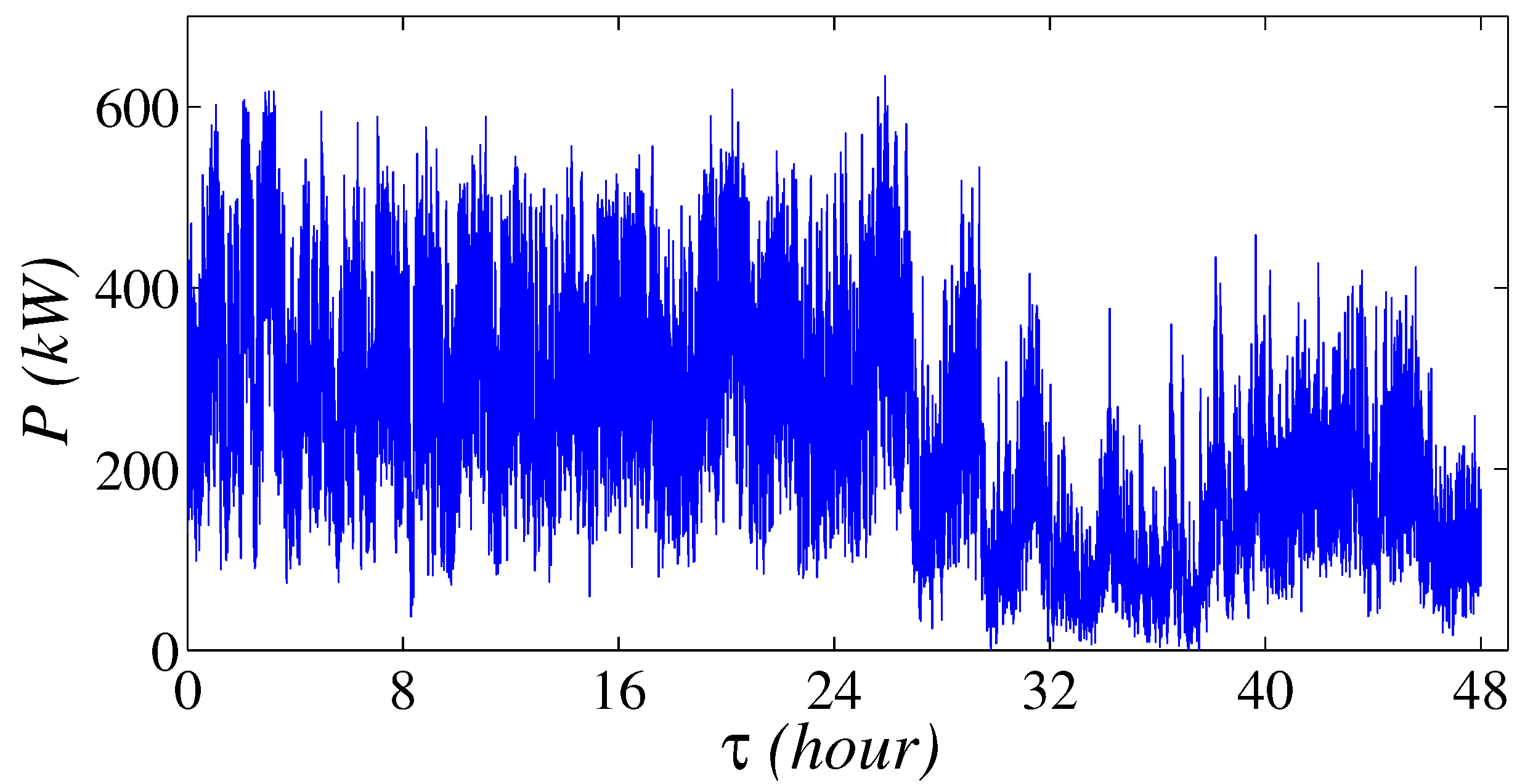
In this study, we consider time series of power output measurements delivered by wind farms and a single turbine. The wind farms are located in the Guadeloupean Archipelago (French West Indies) situated at ${16}^{\circ }{15}^{\prime }$ N latitude and ${60}^{\circ }{30}^{\prime }$ W longitude, in the eastern Caribean sea. The power output measurements delivered by the wind farms labelled $n^{\circ }1$, 2, 3 and 4, are collected continuously with a sampling rate of $T_s=5$ min over more than one year period: this corresponds to $125,942$ data points. These power output data are collected and provided by the French operator of electricity grid Electricité de France (EDF). The power output measurements delivered by the wind farm labelled $n^{\circ }5$, are collected continuously with a sampling rate of $T_s=1$ s during approximately four months: this corresponds to $6,529,000$ data points. The power output measurements from the single turbine, are collected continuously with a sampling rate of $T_s=1$ s during more than six months: this corresponds to $12,257,600$ data points. This wind turbine is located at Risø Campus, Roskilde, Denmark and is a three-bladed stall regulated Nordtank, NTK $500/41$ wind turbine. Figure 1 gives an example of power output delivered by this wind turbine during two days. Table 1 gives a description of following characteristics, sampling frequency, number of continuously data points, implementation site, installed capacity, for each dataset.

Figure 1. An example of power output sequence $p\left(t\right)$ delivered by the single wind turbine during 48 h.

Figure 1. An example of power output sequence $p\left(t\right)$ delivered by the single wind turbine during 48 h.

Table 1. Description of characteristics (sampling frequency, number of continuously data points, implementation site, installed capacity) for each dataset.

Dataset	Sampling Frequency (Hz)	Number of Data Points	Implementation Site	Installed Capacity $P_{\mathrm{inst}}$
Wind farm${}^{\circ }$1	$3.3\times {10}^{-3}$	$125,942$	plateau	2.6 MW
Wind farm${}^{\circ }$2	$3.3\times {10}^{-3}$	$125,942$	plain	2.9 MW
Wind farm${}^{\circ }$3	$3.3\times {10}^{-3}$	$125,942$	plateau	1.9 MW
Wind farm${}^{\circ }$4	$3.3\times {10}^{-3}$	$125,942$	plain	3 MW
Wind farm${}^{\circ }$5	1	$6,529,000$	cliff	10 MW
Single wind turbine	1	$12,257,600$	plain	500 kW

Table 1. Description of characteristics (sampling frequency, number of continuously data points, implementation site, installed capacity) for each dataset.

Dataset	Sampling Frequency (Hz)	Number of Data Points	Implementation Site	Installed Capacity $P_{\mathrm{inst}}$
Wind farm${}^{\circ }$1	$3.3\times {10}^{-3}$	$125,942$	plateau	2.6 MW
Wind farm${}^{\circ }$2	$3.3\times {10}^{-3}$	$125,942$	plain	2.9 MW
Wind farm${}^{\circ }$3	$3.3\times {10}^{-3}$	$125,942$	plateau	1.9 MW
Wind farm${}^{\circ }$4	$3.3\times {10}^{-3}$	$125,942$	plain	3 MW
Wind farm${}^{\circ }$5	1	$6,529,000$	cliff	10 MW
Single wind turbine	1	$12,257,600$	plain	500 kW

3. Taylor Law, a Scaling Relationship between the Mean Value and the Standard Deviation

3.1. Definition of the Taylor Power Law

The study of complex systems in many fields such as ecology, physics, life sciences and engineering sciences [12], has highlighted the universality of the Taylor power law established by L.R. Taylor in 1961 [1]. This relationship has been observed by De Menezes and Barabási with data internet traffic [6] and named later “temporal fluctuation scaling” [10]. Taylor power law is characterized by a relationship between the standard deviation $\sigma =\sqrt{\frac{1}{N-1}{\sum }_{n=1}^{N-1}{(x\left(t\right)-\langle x\rangle )}^2}$ of a signal $x\left(t\right)$ and its mean value $\langle x\rangle =\frac{1}{N}{\sum }_{n=1}^{N}x\left(t\right)$ estimated over a sequence of length N of the considered signal $x\left(t\right)$:

$${\sigma }_{\tau }={\mathcal{C}}_0{\langle x\rangle }^{{\lambda }_{\tau }}$$

(2)

with $\langle .\rangle$ defining the statistical average, $N=L/\tau +1$, L is the total period of the signal $x\left(t\right)$ and τ is the time window corresponding to the time scales explored, ${\mathcal{C}}_0$ is a constant and ${\lambda }_T$ the Taylor exponent.

In this study, the Taylor power law is investigated for the power output data from wind farms and a single wind turbine.

3.2. Taylor Power Law in Wind Energy Data

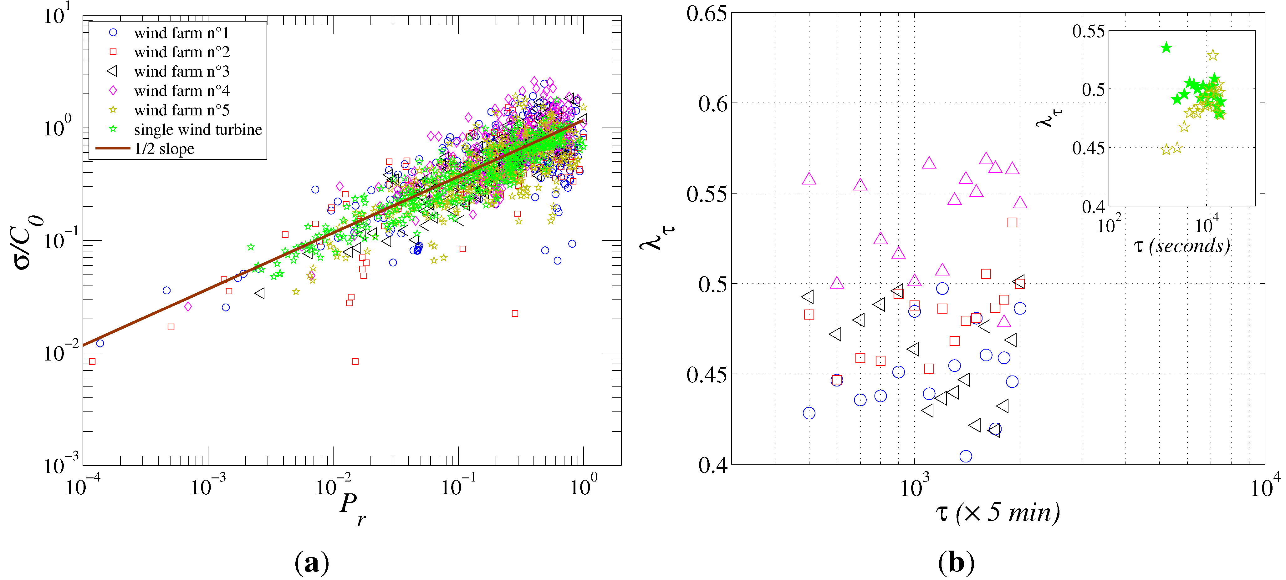
To verify the existence of Taylor power law for our datasets, the mean value ${\langle P\rangle }_{\tau }$ and the standard deviation ${\sigma }_{\tau }$ are computed for time scales (or window sizes) τ ranging between approximately 4 h and 7 days for data sampled at 5 min, and τ ranging between approximately 16 min and 1 day for data sampled at 1 s. The choice of the lower limit of these time intervals is justified by the value of a Pearson correlation $r>0.8$ between the map ($P_r$,${\sigma }_{\tau }/{\mathcal{C}}_0$) and a non parametric kernel smoothing regression fit. Meanwhile, the choice of the upper limit is defined by a time window having a significant sample number for the estimation of the Taylor exponent ${\lambda }_{\tau }$. Hence, each dataset is splitted over a time window of length τ. In Figure 2a, to compare the datasets considered here with the straight line of $1/2$ slope, ${\sigma }_{\tau }/{\mathcal{C}}_0$ versus $P_r$ ($P_r=〈P〉/{〈P〉}_{max}$ with ${〈P〉}_{max}$ the maximum of the mean value for the dataset considered) is illustrated for $\tau =5$ h, in log-log representation. One can observe that the map $(P_r,{\sigma }_{\tau }/{\mathcal{C}}_0)$ can be modeled by a relationship of the form:

$$log\left(\frac{{\sigma }_{\tau }}{{\mathcal{C}}_0}\right)={\lambda }_{\tau }log\left(P_r\right)+c$$

(3)

This leads to a power law of the form

$$\frac{{\sigma }_{\tau }}{{\mathcal{C}}_0}={\left(P_r\right)}^{{\lambda }_{\tau }}$$

(4)

where ${\mathcal{C}}_0={10}^c$.

Figure 2. (a) Evolution of ${\sigma }_{\tau }/{\mathcal{C}}_0$ versus the mean $P_r$. Evolution of the standard deviation ${\sigma }_{\tau }/{\mathcal{C}}_0$ versus the adimensioned mean value $P_r$ for the power output from find wind farms and a single wind turbine. ${\sigma }_{\tau }$ and ${\langle P\rangle }_{\tau }$ are computed with a time window $\tau =5$ h. The map ($P_r$,${\sigma }_{\tau }/{\mathcal{C}}_0)$ is fitted by a non parametric kernel regression (straight line); (b) Evolution of the Taylor exponent ${\lambda }_{\tau }$ versus the time scales τ, for the power output data sampled at five minutes (in the inset for the power output data sampled at 1 s).

Figure 2. (a) Evolution of ${\sigma }_{\tau }/{\mathcal{C}}_0$ versus the mean $P_r$. Evolution of the standard deviation ${\sigma }_{\tau }/{\mathcal{C}}_0$ versus the adimensioned mean value $P_r$ for the power output from find wind farms and a single wind turbine. ${\sigma }_{\tau }$ and ${\langle P\rangle }_{\tau }$ are computed with a time window $\tau =5$ h. The map ($P_r$,${\sigma }_{\tau }/{\mathcal{C}}_0)$ is fitted by a non parametric kernel regression (straight line); (b) Evolution of the Taylor exponent ${\lambda }_{\tau }$ versus the time scales τ, for the power output data sampled at five minutes (in the inset for the power output data sampled at 1 s).

The Taylor exponent whose values correspond to each data set, are drawn up in Table 2. In all the cases, the Taylor power law given in Equation (4) is verified and a scaling behavior is visible over more than four orders of magnitude. Furthermore, the values of ${\lambda }_{\tau }$ are close to $1/2$. To investigate a possible dependence of the exponent ${\lambda }_{\tau }$ with the time scales τ, we plot in Figure 2b, the evolution of the Taylor exponent λ versus the time scale τ for the data sampled at 5 min and in the inset for data sampled at 1 s. One can observe no dependence of the exponent ${\lambda }_{\tau }$ with the time scales τ: it stays between $0.4$ and $0.57$ with a range of variation which does not depend on τ.

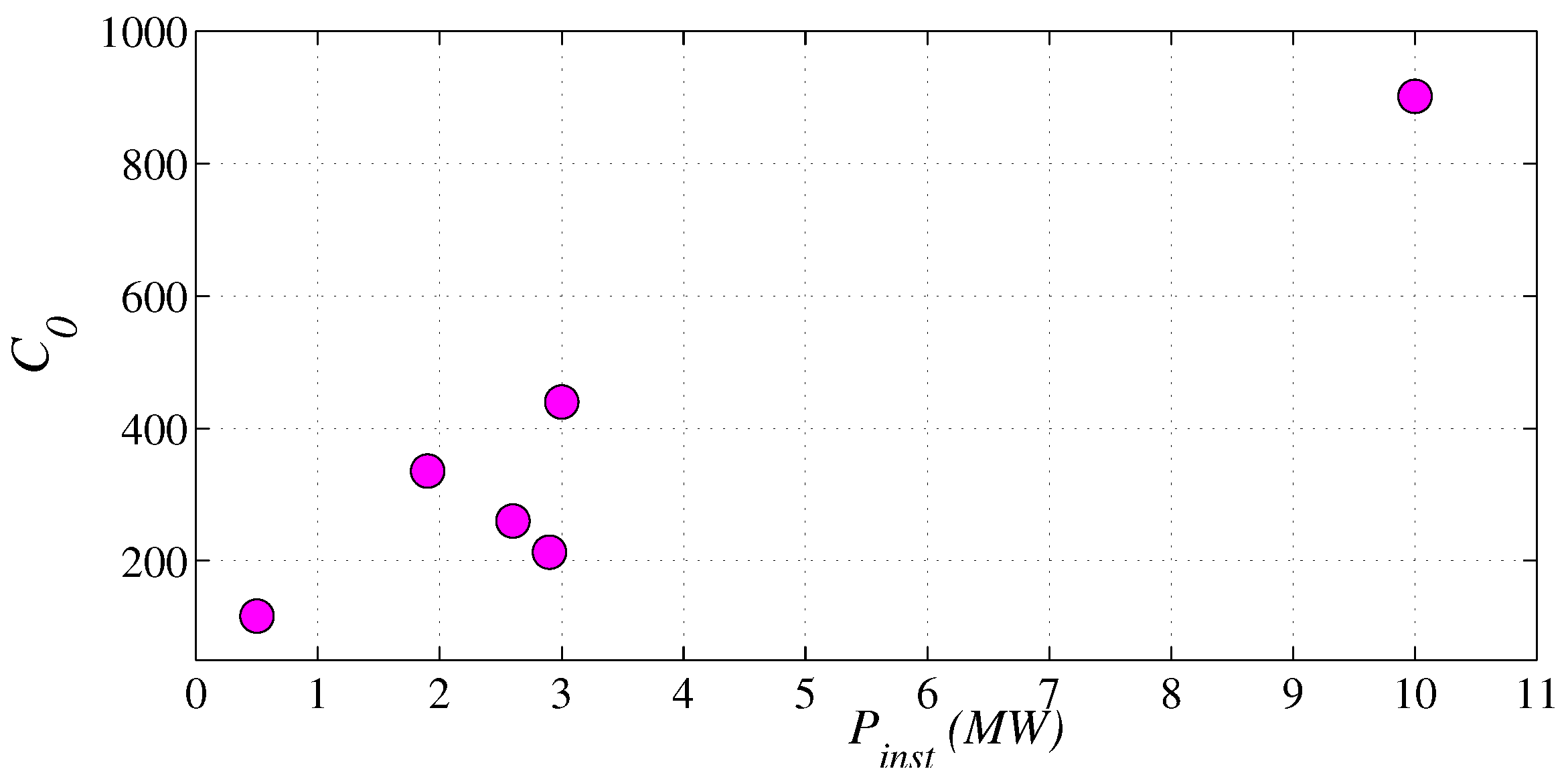
Globally, the Taylor exponent ${\lambda }_{\tau }$ varies between $0.45$ and $0.55$ for times scales τ between 1 h and a one week and ${\mathcal{C}}_0$ can be considered as a parameter characterizing the wind farm or the single turbine considered. Indeed, Figure 3 illustrates the evolution of the parameter ${\mathcal{C}}_0$ versus the installed capacity of the single wind turbine and the wind farms considered. The parameter ${\mathcal{C}}_0$ increases as the installed capacity $P_{inst}$, excepted for the wind farms $n^{\circ }$ 2 and 3 having installed capacities very close.

Table 2. Taylor exponent ${\lambda }_{\tau }$ and ${\mathcal{C}}_0$ estimated for each dataset with $\tau =5$ h: the values obtained are close to $1/2$. ${\mathcal{C}}_0$ can be considered as a parameter characterizing the wind farm or the single turbine considered.

Data	${\lambda }_{\tau }$	${\mathcal{C}}_0$
Wind farm${}^{\circ }$1	$0.48\pm 0.07$	$260.05$
Wind farm${}^{\circ }$2	$0.49\pm 0.07$	$213.05$
Wind farm${}^{\circ }$3	$0.50\pm 0.08$	$335.45$
Wind farm${}^{\circ }$4	$0.55\pm 0.07$	$439.84$
Wind farm${}^{\circ }$5	$0.48\pm 0.05$	$901.57$
Single wind turbine	$0.50\pm 0.05$	$116.41$

Table 2. Taylor exponent ${\lambda }_{\tau }$ and ${\mathcal{C}}_0$ estimated for each dataset with $\tau =5$ h: the values obtained are close to $1/2$. ${\mathcal{C}}_0$ can be considered as a parameter characterizing the wind farm or the single turbine considered.

Data	${\lambda }_{\tau }$	${\mathcal{C}}_0$
Wind farm${}^{\circ }$1	$0.48\pm 0.07$	$260.05$
Wind farm${}^{\circ }$2	$0.49\pm 0.07$	$213.05$
Wind farm${}^{\circ }$3	$0.50\pm 0.08$	$335.45$
Wind farm${}^{\circ }$4	$0.55\pm 0.07$	$439.84$
Wind farm${}^{\circ }$5	$0.48\pm 0.05$	$901.57$
Single wind turbine	$0.50\pm 0.05$	$116.41$

Figure 3. Evolution of parameter ${\mathcal{C}}_0$ versus the installed capacity $P_{inst}$ of the wind farm and the single wind turbine considered.

Figure 3. Evolution of parameter ${\mathcal{C}}_0$ versus the installed capacity $P_{inst}$ of the wind farm and the single wind turbine considered.

3.3. Turbulent Production Intensity $I_P$

Here an analogy is made with the field of the turbulence. Classically, in the turbulence field, a turbulent intensity parameter I expressing the ratio standard deviation to the mean value of the wind speed, is a metric to characterize a turbulence level for flows with high variability, such as wind tunnel or atmospheric wind [21,22,23]. Here this parameter can be used for measuring the degree of variability of the wind power output and for classifying the variability level. In the turbulence field, one can distinguish three classes: (i) $0<I<5\%$ corresponds to a weak level of variability, (ii) $5\%<I<10\%$ corresponds to a medium level of variability and $I>10\%$ corresponds to a high level of variability. In this study, we translate this coefficient to wind power and hence we introduce a new way to measure the variability of wind power data. From the Taylor relationship defined in Equation (4), a scaling relationship between the turbulent production intensity $I_p=\sigma /\langle P\rangle$ and the mean value $\langle P\rangle$, is established by replacing $\langle P\rangle$ by $P_r$:

$$I_p=\frac{\sigma }{P_r}={\mathcal{C}}_0\left(\frac{P_r^{\lambda }}{P_r}\right)$$

(5)

This leads

$$I_p={\mathcal{C}}_0{\left(P_r\right)}^{\alpha }$$

(6)

where the exponent $\alpha =\lambda -1$ is here negative.

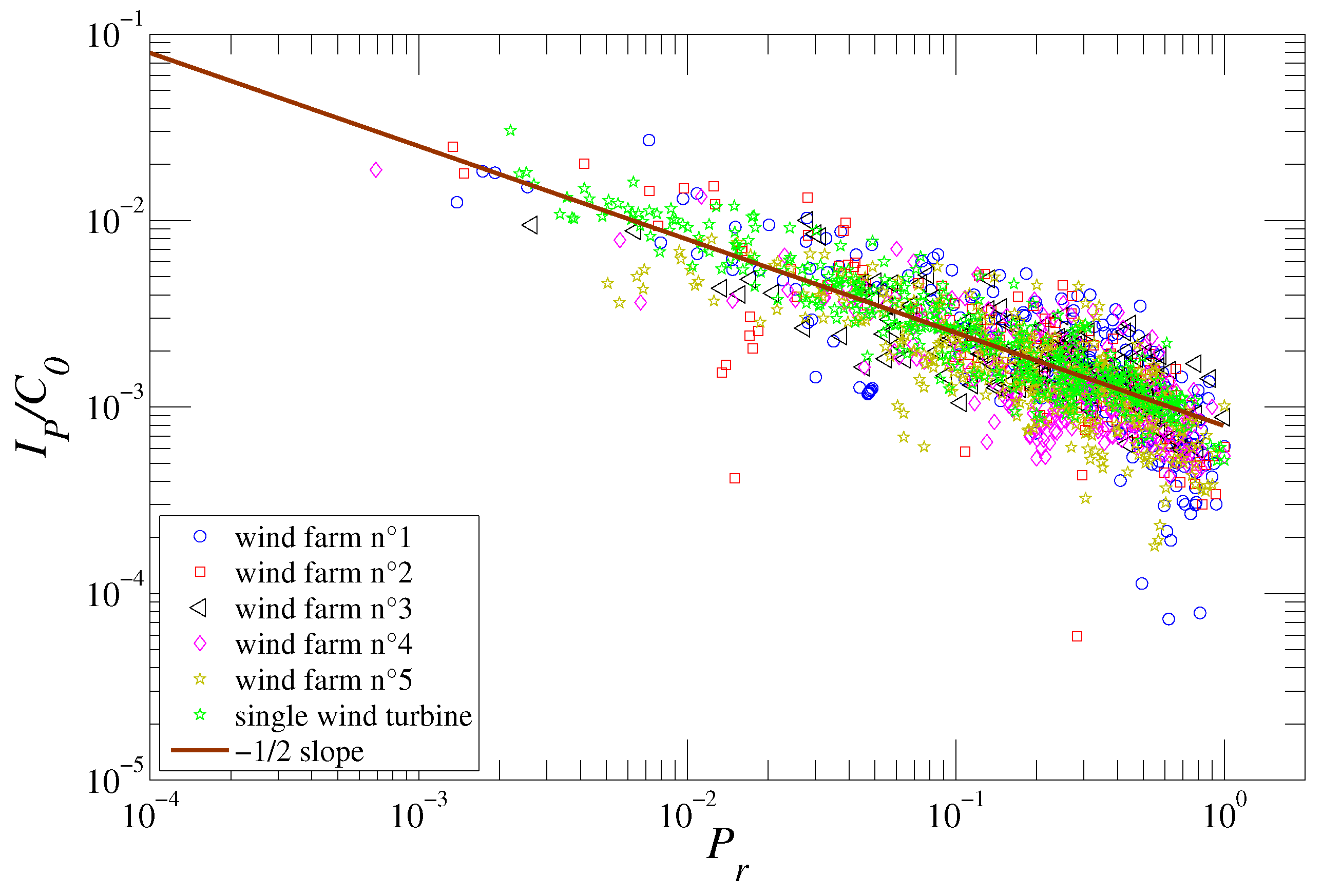
Figure 4 illustrates the evolution of the turbulent production intensity $I_P$ divided by $C_0$ versus the adimensioned mean value $P_r$, in log-log scale. As expected, the turbulent production intensity $I_P$ decreases following a $-1/2$ power law with the mean value $\langle P\rangle$. Hence, taking into account the value obtained for the Taylor exponent ${\lambda }_{\tau }\approx 1/2$, $\alpha \approx -1/2$ for time scales $1h<\tau <7$ days. Table 3 draws up the values of the exponent α estimated for each dataset with $\tau =5$ h. It can be seen that the values are generally corresponding to $I_P>10\%$ which is a very high level of turbulence and that larger values of $P_r$ correspond to smaller values of $I_p$.

Figure 4. Evolution of the adimensioned turbulent production intensity $I_P/{\mathcal{C}}_0$ versus the value $P_r$ compared to the $-1/2$ slope, in log-log scale.

Figure 4. Evolution of the adimensioned turbulent production intensity $I_P/{\mathcal{C}}_0$ versus the value $P_r$ compared to the $-1/2$ slope, in log-log scale.

Table 3. Exponent α estimated for each dataset with $\tau =5$ h.

Data	α
Wind farm${}^{\circ }$1	$-0.48\pm 0.07$
Wind farm${}^{\circ }$2	$-0.49\pm 0.07$
Wind farm${}^{\circ }$3	$-0.50\pm 0.08$
Wind farm${}^{\circ }$4	$-0.55\pm 0.05$
Wind farm${}^{\circ }$5	$-0.48\pm 0.05$
Single wind turbine	$-0.50\pm 0.05$

Table 3. Exponent α estimated for each dataset with $\tau =5$ h.

Data	α
Wind farm${}^{\circ }$1	$-0.48\pm 0.07$
Wind farm${}^{\circ }$2	$-0.49\pm 0.07$
Wind farm${}^{\circ }$3	$-0.50\pm 0.08$
Wind farm${}^{\circ }$4	$-0.55\pm 0.05$
Wind farm${}^{\circ }$5	$-0.48\pm 0.05$
Single wind turbine	$-0.50\pm 0.05$

4. Conclusions and Discussions

In this study, we have investigated the existence of a Taylor power law or temporal fluctuation scaling of power output delivered by five wind farms and a single wind turbine, with different installed capacity. The analyzed data are sampled at 1 s and five minutes, and recorded over different periods. A Taylor power law has been highlighted for all the datasets. Furthermore, a universal scaling exponent ${\lambda }_{\tau }$ close to $1/2$, is observed for time scales $1h<\tau <7$ days for the data sampled at 5 min, and $5min<\tau <6$ h for the data sampled at 1 s.

The existence of such Taylor law has been shown in multiple disciplinary fields. This universality has conducted many authors to suggest the existence of a universal mechanism for its emergence. Various approaches and theoretical investigations have been dedicated to possible explanations of the origin of Taylor law. In the framework of a complex systems whose dynamics is the result of interactions of many components belonging to a network [6,7], the value of λ gives an information on the mechanism governing the fluctuations involved in the process: $\lambda \approx 1/2$ describes processes or systems where internal factors drive dynamics and $\lambda \approx 1$ describes processes where external factors drive the dynamics [6,7,8]. This was investigated for internet traffic data and complex networks [6,7,8]. This result was experimentally based and cannot be used for understanding wind energy dynamics. Recently, Fronczak and Fronczak (2010) [24] attempted to provide an interpretation of Taylor’s relation based on the second law of thermodynamics (the maximum entropy principle) and the number of states. Kendal and Jørgensen (2011) [25] proposed the Tweedie Convergence Theorem to give a possible explanation of the origin of Taylor law. They show that Tweedie convergence theorem, a generalization of Central Limit Theorem, provides an explanation for the genesis of Taylor laws. They also showed that Taylor law is a scaling relationship, compatible with the presence $1/f$ scaling and multifractal properties, characteristic of a self-similar process. On the other hand, several authors have shown the presence of $1/f$ scaling [26] and recently multifractal properties for wind energy data [20,27,28,29]. A way to highlight multifractal properties is the use of a multi-scaling analysis including $q^{th}$- order central moments versus the mean value, a natural generalization of Taylor law where $q=2$, or multifractal analysis [8,27,29]. Although the Tweedie Convergence Theorem seems offer a promising explanation, there is currently no generally accepted theory to explain the emergence of Taylor’s relation.

The existence of Taylor’s law with $1/2$ exponent should help to provide an estimation of the mean fluctuations for a mean value fixed of wind power data, but also to propose a statistical model of wind power data using Tweedie model PDF. Our findings may be useful for developers and operators of wind parks.

References

- Taylor, L.R. Aggregation, variance and the mean. Nature 1961, 189, 732–735. [Google Scholar] [CrossRef]
- Smith, H.F. An empirical law describing heterogeneity in the yields of agricultural crops. J. Agric. Sci. 1938, 28, 1–23. [Google Scholar] [CrossRef]
- Keitt, T.H.; Stanley, H.E. Dynamics of North American breeding bird populations. Nature 1998, 393, 257–260. [Google Scholar] [CrossRef]
- Kerkhoff, A.J.; Ballantyne, F. The scaling of reproductive variability in trees. Ecol. Lett. 2003, 6, 850–856. [Google Scholar] [CrossRef]
- Xu, M.; Schuster, W.S.; Cohen, J.E. Robustness of Taylor’s law under spatial hierarchical groupings of forest tree samples. Popul. Ecol. 2015, 103, 1–11. [Google Scholar] [CrossRef]
- De Menezes, M.; Barabási, A.L. Fluctuations in Networks Dynamics. Phys. Rev. Lett. 2004, 92, 028701. [Google Scholar] [CrossRef] [PubMed]
- De Menezes, M.; Barabási, A.L. Separating Internal and External Dynamics of Complex Systems. Phys. Rev. Lett. 2004, 93, 068701. [Google Scholar] [CrossRef]
- Eisler, Z.; Kertész, J.; Yook, S.G.M.; Barabási, A.L. Multiscaling and non-universality in fluctuations of driven complex systems. Europhys. Lett. 2005, 69, 664–670. [Google Scholar] [CrossRef]
- Eisler, Z.; Kerész, J. Random walks on complex networks with inhomogeneous impact. Phys. Rev. E 2005, 71, 057104. [Google Scholar] [CrossRef]
- Eisler, Z.; Kertész, J. Scaling theory of temporal correlations and size-dependent fluctuations in the traded value of stocks. Phys. Rev. E 2006, 73, 040109. [Google Scholar] [CrossRef]
- Šuvakov, M.; Tadić, B. Transport processes on homogeneous planar graphs with scale-free loops. Phys. A 2006, 372, 354–361. [Google Scholar] [CrossRef]
- Eisler, Z.; Bartos, I.; Kertész, J. Fluctuation scaling in complex systems: Taylor’s law and beyond. Adv. Phys. 2008, 57, 89–142. [Google Scholar] [CrossRef]
- Lee, Y.; Amaral, L.A.N.; Canning, D.; Meyer, M.; Stanley, H.E. Universal features in the growth dynamics of complex organizations. Phys. Rev. Lett. 1998, 81, 3275–3278. [Google Scholar] [CrossRef]
- Jiang, Z.Q.; Guo, L.; Zhou, W.X. Endogenous and exogenous dynamics in the fluctuations of capital fluxes: An empirical analysis of the Chinese stock market. Eur. Phys. J. B 2007, 57, 347–355. [Google Scholar] [CrossRef]
- Jánosi, I.M.; Gallas, J.A. Growth of companies and water-level fluctuations of the river Danube. Phys. A 1999, 271, 448–457. [Google Scholar] [CrossRef]
- Dahlstedt, K.; Jensen, H.J. Fluctuation spectrum and size scaling of river flow and level. Phys. A 2005, 348, 596–610. [Google Scholar] [CrossRef]
- Azevedo, R.B.; Leroi, A.M. A power law for cells. Proc. Natl. Acad. Sci. 2001, 98, 5699–5704. [Google Scholar] [CrossRef] [PubMed]
- Nacher, J.C.; Ochiai, T.; Akutsu, T. On the relation between fluctuation and scaling-law in gene expression time series from yeast to human. Mod. Phys. Lett. B 2005, 19, 1169–1177. [Google Scholar] [CrossRef]
- Kendal, W.S. An exponential dispersion model for the distribution of human single nucleotide polymorphisms. Mol. Biol. Evol. 2003, 20, 579–590. [Google Scholar] [CrossRef] [PubMed]
- Calif, R.; Schmitt, F.G. Analyse de séries temporelles de production éolienne: Loi de Taylor et propriétés multifractales. In Compte Rendu de la 15e Rencontre du Non-Linéaire; Falcon, E., Josserand, C., Lefranc, M., Letellier, C., Eds.; Non-Linéaire Publications: Paris, France, 2012; pp. 61–66. [Google Scholar]
- Pope, S.B. Turbulent Flows; Cambridge University Press: Cambridge, UK, 2000; p. 792. [Google Scholar]
- Petersen, E.K.; Mortensen, N.G.; Landberg, L.; Højstrup, J.; Frank, H.P. Wind power meteorology. Wind Energy 1999, 1, 25–45. [Google Scholar] [CrossRef]
- Calif, R.; Emilion, R.; Soubdhan, T. Classification of wind speed distributions using a mixture of Dirichlet distributions. Renew. Energ. 2011, 36, 3091–3097. [Google Scholar] [CrossRef]
- Fronczak, A.; Fronczak, P. Origins of Taylor’s power law for fluctuation scaling in complex systems. Phys. Rev. E 2010, 81, 066112. [Google Scholar] [CrossRef]
- Kendal, W.S.; Jørgensen, B. Tweedie convergence: A mathematical basis for Taylor’s power law, 1/f noise, and multifractality. Phys. Rev. E 2011, 84, 066120. [Google Scholar] [CrossRef]
- Apt, J. The spectrum of power from wind turbines. J. Power Sources 2007, 169, 369–374. [Google Scholar] [CrossRef]
- Calif, R.; Schmitt, F.G.; Huang, Y. The multifractal description of wind power fluctuations using arbitrary order Hilbert spectral analysis. Phys. A 2013, 392, 4106–4120. [Google Scholar] [CrossRef]
- Milan, P.; Wächter, M.; Peinke, J. Turbulent character of wind energy. Phys. Rev. Lett. 2013, 110, 138701. [Google Scholar] [CrossRef] [PubMed]
- Calif, R.; Schmitt, F.G. Multiscaling and joint multiscaling description of the atmospheric wind speed and the aggregate power output from a wind farm. Nonlinear Proc. Geophys. 2014, 21, 379–392. [Google Scholar] [CrossRef] [Green Version]
© 2015 by the authors; licensee MDPI, Basel, Switzerland. This article is an open access article distributed under the terms and conditions of the Creative Commons Attribution license (http://creativecommons.org/licenses/by/4.0/).
Share and Cite
MDPI and ACS Style
Calif, R.; Schmitt, F.G. Taylor Law in Wind Energy Data. Resources 2015, 4, 787-795. https://doi.org/10.3390/resources4040787
AMA Style
Calif R, Schmitt FG. Taylor Law in Wind Energy Data. Resources. 2015; 4(4):787-795. https://doi.org/10.3390/resources4040787
Chicago/Turabian StyleCalif, Rudy, and François G. Schmitt. 2015. "Taylor Law in Wind Energy Data" Resources 4, no. 4: 787-795. https://doi.org/10.3390/resources4040787