Building Robust Housing Sector Policy Using the Ecological Footprint

1
School of Environmental and Life Sciences, Discipline of Geography, Bldg SRR, University of Newcastle, Callaghan, NSW 2308, Australia
2
Integrated Sustainability Analysis, School of Physics A28, University of Sydney, Sydney, NSW 2006, Australia
3
School of Geosciences, University of Sydney, Madsen Building (F09), Room 348, Eastern Avenue, Sydney, NSW 2006, Australia
4
Global Footprint Network, 312 Clay Street, Suite 300, Oakland, CA 94607-3510, USA
*
Author to whom correspondence should be addressed.
Resources 2018, 7(2), 24; https://doi.org/10.3390/resources7020024
Submission received: 9 February 2018
/
Revised: 15 March 2018
/
Accepted: 20 March 2018
/
Published: 23 March 2018
(This article belongs to the Special Issue Ecological Footprint Assessment for Resources Management)
Abstract
:The vulnerability of the urban residential sector is likely to increase without the mitigation of growing household Ecological Footprints (energy demand, CO2 emissions, and demand for land). Analysis comparing the effectiveness and robustness of policy to mitigate the size of the housing Ecological Footprint has been limited. Here, we investigate three mitigation options: (1) reducing housing floor area, (2) improving the building envelope efficiency, and (3) reducing the carbon intensity of the electricity sector. We model the urban residential Ecological Footprint for a sub-national case study in Australia but analyse the results in the global context. We find that all three mitigation options reduce the Ecological Footprint. The success of policy to reduce household energy demand and land requirements is somewhat dependent on uncertain trajectories of future global population, affluence, and technological progress (together, global uncertainty). Carbon emissions reductions, however, are robust to such global uncertainty. By reducing the Ecological Footprint of the urban residential housing sector we see a reduction in its vulnerability to future global uncertainty, global carbon price, urban sprawl, and future energy shortages. Over the long term, such policy implementation can also be highly cost effective.
Highlights:
- We modelled the Ecological Footprint of operational energy of urban residential housing
- We tested three mitigation options for reducing this Ecological Footprint
- Mitigation effectively reduced energy demand, CO2 emissions, and land requirements
- The success of energy policy and land demand were somewhat vulnerable to future global uncertainty
- CO2 emission reductions were robust to future global uncertainty
1. Introduction
The Ecological Footprint is an indicator which can be used to track the consumption of land and/or biotic resources and the carbon based waste of human populations. The global Ecological Footprint of built land continues to increase [1] as world populations become more urbanised. Furthermore, 40–50% of global greenhouse gas emissions originate from buildings [2].
Operational energy (the energy that is used in a house to function day to day), by far, accounts for the majority of the energy over the lifetime of an ‘average’ residential building [3,4]. Reducing the operational energy of a building, however, means that embodied energy (the energy used to build the building) becomes a more significant proportion of overall building energy requirements. For example, for a typical house in Scandinavia with a lifetime of 50 years, the proportion of embodied energy is about 10 ± 15% of the operational energy. In comparison, the embodied energy of a low energy house accounts for as much as 60% of the total energy use [3].
Although it is possible that more embodied energy is required (e.g., to incorporate greater thermal mass and insulation in a building) than is saved through reduced operational energy; most research has found the additional investment in embodied energy is small relative to the energy savings over the lifetime of the building [4]. Therefore, at least initially, reducing the operational energy of the building sector is the most important focus for reducing the environmental impact of the housing sector. Embodied energy should then be addressed in the second instance.
The operational energy of the urban housing sector is likely to continue to increase in response to increasing household income, household floor area, and urban population growth [5]. Rises in energy demand will make many households more vulnerable to rising energy prices and future energy shortages [6,7]. Increases in carbon emissions could also increase the vulnerability of households to the introduction of a carbon price [8]. Lastly, continued demand for urban land will exacerbate the vulnerability of households associated with urban sprawl [9].
However, the potential to mitigate environmental impacts of the sector also appears to be high. Watson, et al. [10], for instance, estimated that the domestic and commercial buildings sector globally has the potential to halve emissions by 2054.
Barker et al. note that substantial CO2 emission reduction from energy use in buildings can be achieved over the coming years [11]. About seventy percent of technologies necessary to significantly reduce emissions with building efficiency already exist [12,13]. In individual new buildings, it is possible to achieve 75% or more energy savings compared with recent current practice, generally at little or no extra cost [11].
Substantial savings in energy from buildings are possible largely through efficient lighting technologies, improved insulation and heating in the colder climates, efficiency measures related to space cooling and ventilation in the warmer climates, solar water heating, integrated building design, passive solar construction, and energy-management systems [11,14].
The objective of this study was to investigate the effectiveness of three policy levers (reducing housing floor area, improving the building envelope efficiency of housing stock, and reducing the carbon intensity of the electricity sector) to reduce the future vulnerability of the residential housing sector. To understand changes in vulnerability, we measured three factors that contribute to the Ecological Footprint: operational energy, CO2 emissions, and land requirements. We examine the effectiveness of these policy options at a sub-national scale using a case study state in Australia (Queensland); however, the global context is also included as it is considered integral to the success of local policy development. We used scenario analysis to investigate: (1) future uncertainty related to trajectories of population, affluence, and technological progress and (2) global carbon price to understand implications for local housing sector vulnerability.
The findings of our local analysis have policy implications for other geographical localities because the trends evident in Australia of increasing urban populations, increasing house size, and lower occupancy per household are mirrored globally.
2. Methods
In the following section, we outline the approach taken to investigate the Ecological Footprint for the housing sector and the effectiveness of mitigation options to reduce the future Footprint. We outline the broader Ecological Footprint model within which we undertook more detailed modelling for the housing sector, we describe how we incorporate the global context and its inherent uncertainties, we describe the regional policy setting, we describe and justify the variables specific to the housing component of our model, and, finally, we describe the approach we took to investigate mitigation options and their timing.
2.1. The Model
The modelling of the urban residential housing sector, as described in this paper, sits within the context of a larger global model that estimates future Ecological Footprints and Biocapacity at a national scale for 116 countries. This model is described in more detail in [15,16]. At its basis, this model has an IPAT (Environmental Impact is influenced by Population, Affluence and Technology) formulation (environmental impact is assumed to be influenced by the drivers population, affluence, and technology). These drivers determine the land requirement (built, cropping, grazing, plantation, forest) and CO2 emissions (the net emissions produced from the stationary energy sector, the transport sector [17], agricultural emissions, land clearing, and forest sequestration), which can be aggregated to calculate the Ecological Footprint and Biocapacity. The mathematical structure of the model is described in Lenzen and McBain [18].
Our model consists of a 6-dimensional tensor structure that allows non-linear cause-and-effect relationships to occur:
- between different variables (e.g., increases in population may drive an increase in demand for cropping land),
- between different nations (e.g., CO2 emissions from one location affect changes in climate in another location),
- from impacts that occur historically (e.g., CO2 emissions from historical land clearing continue to impact climate in the present time due to its long half-life in the atmosphere).
Variables are advanced in annual time steps based on specific non-linear cause-and-effect relationships between a variable and its key drivers. Data for key drivers comes from the previous time step in the model (or historical data). For example, population and per capita income are the key drivers of the extent of urban land in each country. The national area of urban land is calculated by multiplying country specific coefficients with data for population and per capita income from the previous modelled time-step. In our model, both population and per capita income both happen to be exogenous data that come from the Intergovernmental Panel on Climate Change Special Report on Emissions Scenarios (IPCC SRES) scenarios, see Section 2.2 below. However, data for key drivers used to progress a variable to the next annual time-step can also be endogenously calculated within the model itself. For example, the extent of urban land (calculated within our model as above) will then be used as data to calculate the number of households in a country (as described in more detail below in Section 2.4.1).
2.2. The Global Context
The future trajectories of the IPAT drivers, which form the basis of our modelling framework, are highly uncertain. To describe this future global uncertainty, we used three Intergovernmental Panel on Climate Change Special Report on Emissions Scenarios (IPCC SRES scenarios: A2r, B1, and B2). These scenarios constitute future trajectories that are distinctly different and encompass a significant portion of the underlying uncertainties in the main driving forces that determine future Ecological Footprints. The two key future uncertainties that the SRES scenarios have identified are: (1) the degree to which world values emphasise economic growth over greater balance between economic and environmental considerations (labelled as either A or B, respectively) and (2) the degree to which institutional and economic interactions are globally integrated or become more regionally isolated (labelled 1 or 2). The assumptions behind these scenarios influence the trajectories of future population, affluence, and technological progress. The scenarios can be characterised briefly as follows:
- A2r: high population, medium-low income growth, low technology growth;
- B1: medium-high population, medium income growth, high technological growth;
- B2: low population, high income growth, medium technological growth.
It is important to note that the trajectories of population, affluence, and technology do not progress independently, and their interactions are a critical consideration in the development of these scenarios. Population and Gross Domestic Product (GDP) data were sourced from the Greenhouse Gas Initiative (GGI) Scenario database [19,20] and served as exogenous data in our modelling.
2.3. The Regional Context
In contrast to this global context, it is at the national and regional scale where policy influences the environmental impact of the housing sector. We use a case study state, Queensland in Australia, to investigate the policy options available to regional policy makers to reduce the vulnerability of the residential housing sector. Energy use and CO2 emissions from the Australian buildings sector range from 10–27% and 12% of total national energy and emissions, respectively [21,22]. In Australia, trends in building efficiency indicate modest recent improvements in building efficiency from 280 to 200 MJ/m2 [23]. Unfortunately, the improvement in building shell efficiency has been outpaced by the rate of increase in average floor area. As a result, the potential space conditioning load is estimated to have increased from 30 GJ to 35 GJ per household per annum from 1986 to 2005 [23]. With a current housing stock with: (1) large reliance on an electricity sector which is heavily fossil fuel based; (2) large house sizes by international standards; and (3) low building envelope efficiency, the Australian population is highly vulnerable to future energy price increases and climate variability.
2.4. Urban Residential Housing Model Variables and Algorithms
Below we outline and justify the variables included within the urban residential housing part of our larger global Ecological Footprint model. We describe how modelling is undertaken and detail data sources. The choice of variables in the model was determined from a review of the literature (also included below).
We estimate the first three variables (number of households, floor area, and household size) globally as well as for our case study to set the global context and to establish the relevance and applicability of this model beyond Australia. The remaining variables are estimated for our Australian case study only.
2.4.1. Number of Households
Although total population is an important driver of environmental impact, the number of households is far more informative for estimating housing sector environmental impacts. Data from the UN-Habitat Urban and Housing Indicators database [24] for urban population and number of people per household were used to calculate the number of households within each of over 200 cities located throughout the world. We calculated the relationship between the number of households and its determinants, urban density, and total urban population, using multiple regressions for cities categorised by development. The result of the regression can be found in Table 1 and these form the variable used in our model.
2.4.2. Floor Area
The floor area of housing stock is an important determinant of environmental impact. Hu, Van Der Voet, and Huppes [5] note that, globally, average floor area of housing stock can be an indicator of living standards, where low average floor area indicates overcrowding and higher areas, an improvement in living standards. However, increases in floor area also result in greater energy and material requirements of housing (once a certain standard of living is achieved above and beyond an ‘adequate’ floor area). We applied the logarithmic relationship (y = 6.33Ln(x) − 28.95, R2 = 0.81) presented in Isaac and Van Vuuren [25] to determine floor space based on GDP per capita (x) for each of the world’s countries.
As noted by Isaac and Van Vuuren [25], the trends for housing area in the USA, Canada, and Australia do not follow this international relationship (i.e., they are outliers). Therefore, we undertook further investigation of floor area in Australia and its states. Historical data for average housing stock residential dwelling floor area by state [23] show linear increases in housing floor area from 32–41 to 55–64 over the two decades prior to 2006.
It is clear that such linear increases cannot occur indefinitely because of limits to house block sizes which will ultimately physically restrict further growth. In addition, there are also future limitations due to housing affordability since larger houses cost more and will require greater expenditure to heat, cool, furnish, clean, etc. However, average housing area can continue to increase somewhat in the future due to renovation of old stock, which extends floor area. DEWHA [23] assumed a decline in the average floor area for a new detached dwelling from approximately 250 m2 (2005 national average) down to 230 m2 (i.e., down to 92%) by 2009 and that the area will stabilise at this level in the foreseeable future beyond 2009. However, it is also noted that future trends in floor area are highly uncertain.
We have made the assumption that house size stabilises to the average current household size in each state +10% by 2030. This assumes that new house size plateaus from the present onwards, but retrofitting of older houses results in an increase in the average value until 2030.
2.4.3. Household Size
The average household size (number of people living in each household) in developed countries fell from around 3.6 in 1950 to 2.7 people per household in 1990. This rapid decline can largely be accounted for by ageing, rising divorce rates, rising age at marriage, and increasing childlessness. Household size in developing countries that currently have high fertility actually increased between 1950 and 1996 [26]. We derived the following logarithmic relationship for household size and per capita GDP using data from UN Habitat (household size = −0.8027Ln(GDP) + 10.161, R2 + 0.5).
2.4.4. Housing Lifetime
The lifetime of housing varies greatly from 30 and 100 years [4]. Buildings are often demolished because they are located in the wrong place, not because they are technically worn out [3]. Kapambwe, et al. [27] found that the average lifespan of dwellings for Australia was 61 years (range 45–73). Houses were demolished for the purposes of site redevelopment (58%), the building ceasing to suit owners’ requirements (28%), the dwelling becomes unserviceable (8%), and damage by fire, storm, etc. (6%). We assumed a maximum building lifetime of 100 years but adjusted average lifetime based on state specific data. We assumed a normal distribution for the age of housing stock.
2.4.5. Star Rating
The Australian National House Energy Rating Scheme (NatHERS) was introduced in 2003. The energy consumption per unit area (KWh/m2) for each star rating varies geographically across Australian states, i.e., the same star rating in one state will have different energy use per m2 than in another state.
Building shell energy efficiency in Australia has improved somewhat since the 1980s from 280 to 200 MJ/m2. We derived the following state specific relationship between energy per unit area (y) and the NatHERS start rating (x) for our modelling for Queensland (y = −32.46Ln(x) + 81.492). We assume that the average star rating for housing in Queensland in 1990 was 1 [28]. Emissions per m2 for housing previous to this date are also assumed to have the equivalent of a 1-star rating. The National Strategy on Energy Efficiency [29] requires a minimum six-star energy rating (or equivalent) for new homes built from 2011. Therefore, we assume a star rating of 8 for the average new house by 2100 under little additional mitigation policy.
2.4.6. Housing Fuel Mix
Residential fuel mix between 1990 and 2005 (electricity, charcoal, natural gas, fuelwood, and coal) was calculated from data obtain from UN Statistical Division. Data for Australian states was obtained from Australian Bureau of Agriculture and Resource Economics (ABARE, for natural gas and electricity). Energy mix for 2100 was assumed to be 100% electricity. The assumptions behind the future fuel mix of the electricity sector, with no specific mitigation of CO2 emission, are documented in McBain et al. (unpublished).
For Australia, the main sources of energy used by urban residents are in the form of gas, electricity, and fuel for vehicles, with other forms of energy being negligible (e.g., heating oil, wood, bottled gas) [21]. The use of wood heating is assumed to decline under increasing regulation of air pollution. Although the use of natural gas for heating and hot water has increased in recent times in Australia [30], it is seen as a transitional fuel and is assumed to be fully replaced by renewable sources of electricity by 2100.
The CO2 emission factor from residential natural gas combustion was sourced from the National greenhouse accounts factors (51.2 kg CO2-e/GJ or 1.4222 × 10⁻⁵ MT CO2-e/KWh).
The emission factor for direct energy from natural gas is assumed to remain constant into the future. Should efficiency gains occur, this should not significantly affect the policy outcomes of the model, since we assume direct energy use of natural gas in the residential setting is phased out by 2100 to be replaced by electricity.
2.4.7. Carbon Intensity of Electricity Sector
We also consider the effect of lowering the carbon intensity of the electricity sector by reducing fossil fuels in the future fuel mix as modelled in detail in McBain et al., unpublished. The technologies considered include efficient base load coal plants; gas base load power replacing coal power; capture of CO2 at base load power plant (CCS coal or natural gas); and wind, solar photovoltaic (PV), nuclear, biomass, hydro, concentrated solar power (CSP), and geothermal replacing coal power. We calculated the carbon intensity of the electricity sector by applying emission factors for each stationary energy technology using data from Lenzen and Schaeffer [31] and adjusting for each SRES scenario [32] as detailed in Table 2.
2.5. Mitigation Options
A review of Queensland government policy documents related to climate change indicate that changing urban form and improved building efficiency are priority approaches targeted for policy action. Strategies for reducing the carbon footprint of Queensland are outlined in the Climate Change Strategy. This highlights the role of a more compact and interconnected urban form called Transit Orientated Development (TOD) to reduce emissions from vehicles and increase the use of public transport and active transport. Adopting more appropriate urban form may also result in co-benefits (or at least not negative impacts) for the construction industry since significant redevelopment will be required.
Water heating and air conditioning accounts for the majority of the average Queensland household’s 13.77 tonnes of greenhouse gas produced per year. Electricity usage has increased by 10% per annum in recent years [33].
The 33,000 new houses projected to be built every year in Queensland until 2026 [33] are an opportunity, e.g., through improved building standards, to reduce environmental impact and decrease the vulnerability of the housing sector. However, these new developments represent only 2% of the total building stock each year [33]. Therefore, retrofitting the existing housing stock is of prime importance. Improving housing efficiency can be undertaken at low cost or with net benefit to the economy [13].
2.5.1. Household Floor Area
For the purposes of mitigating average household floor area, we made the assumption that house size stabilises by returning to the current average household size in each state by 2030. This assumes that new house sizes plateau and there are policy incentives to slow renovations of older houses that increase floor area. These trends, together with (1) high density developments around urban transport nodes and (2) other incentives for replacing existing housing stock with smaller buildings is assumed to result in a reduction in average house size to 1990 levels by 2060.
2.5.2. Star Rating
An average star rating of 8 and 10 is presumed by 2100, under scenarios of no mitigation and implementation of mitigation to increase housing envelope efficiency, respectively.
2.5.3. Rate of Technological Uptake
We increase the proportion of houses with a chosen star rating by decreasing the average housing lifetime (i.e., skewing the normal distribution presumed for housing age to the right). We assumed an average house age of 35–50 years and 25 years under scenarios with no mitigation and mitigation, respectively.
2.5.4. Reducing the Carbon Intensity of the Electricity Sector
We consider the effect of lowering the carbon intensity of the electricity sector by reducing fossil fuels in the future fuel mix as modelled in detail in McBain et al., unpublished, as summarised in Table 3.
2.6. Components of the Ecological Footprint
2.6.1. Operational Energy
We calculated the total operational energy of the housing sector by multiplying the energy consumption per unit area (KWh/m2) for the appropriate star rating by the total household area.
2.6.2. CO2 Emissions
We used CO2 emissions as our proxy for the carbon waste fraction of the Ecological Footprint. We multiplied the emission factors (Table 1) with the total stationary energy produced for each technology according to the fuel mix specified in Table 3. We implemented scenario specific change in emission intensity by calculating the rate of change between 2009 and 2100 and used this rate to adjust our emission factor each year.
2.6.3. Total Household Floor Area
We used total household floor area as our proxy for the urban land component of the Ecological Footprint. We calculated total household floor area by multiplying the average household floor area by the total urban population.
3. Results
Globally, urban populations will continue to increase (Figure 1a). The residential household floor area per person is also likely to increase with increasing affluence (Figure 1c). This increase in affluence also means that the number of people living within each household is likely to decrease (Figure 1b). These trends mirror those occurring in our Queensland case study, indicating that our case specific policy findings have broader international applicability. This is especially relevant in areas where affluence and urban population continues to increase rapidly.
The sub-national results for Queensland are shown (Figure 2, Figure 3 and Figure 4) to demonstrate the typical changes in operational energy, CO2 emissions, and total land requirement of the residential housing sector that may occur within the above global context.
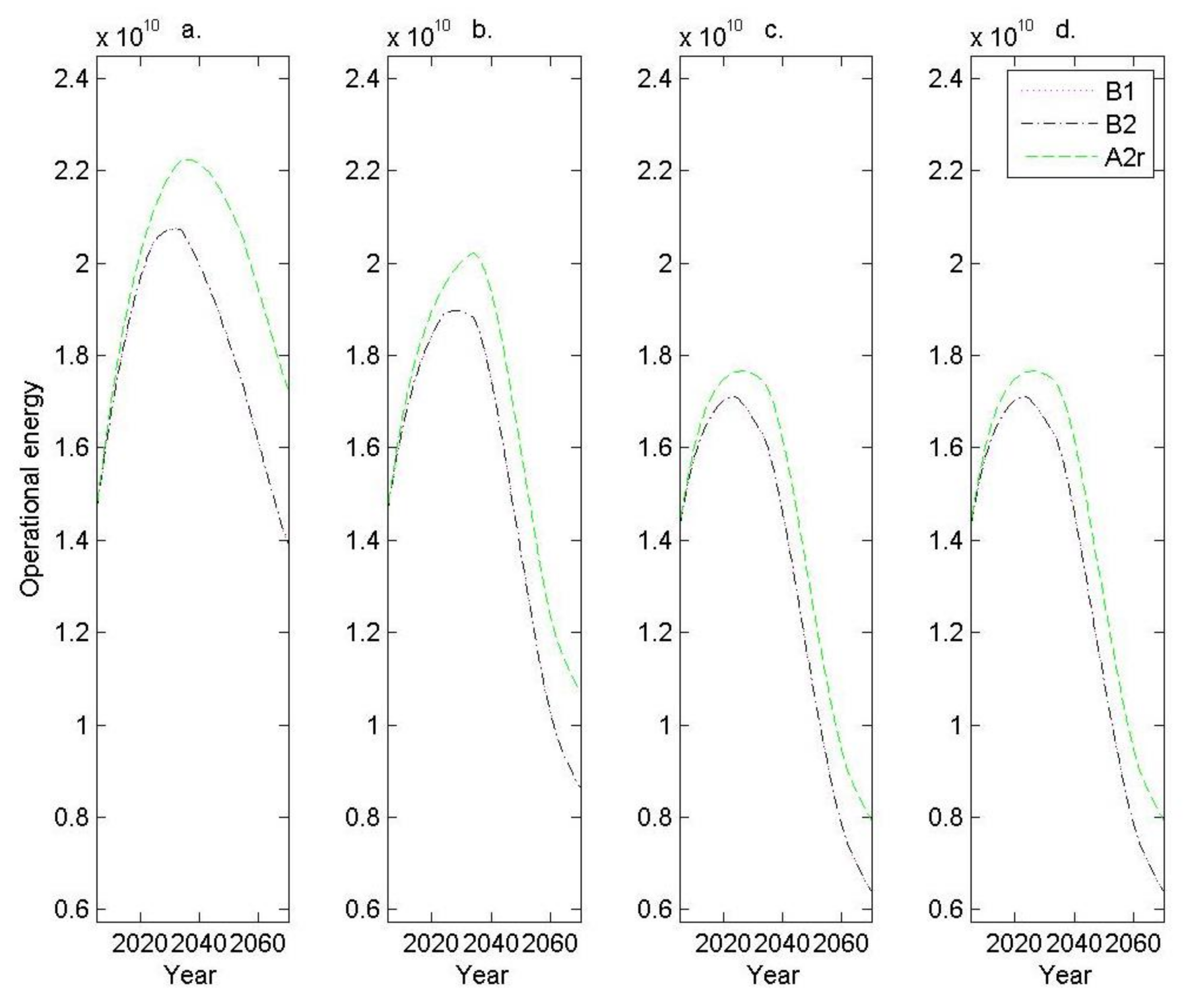
The combined influence of population growth, growth in GDP per capita, and varying degrees of technological uptake all mean that the household energy demand (Figure 3) varies under the influence of different global scenarios with the highest energy demand under an A2r future, and somewhat lower demand under B1 or B2. Under an A2r scenario, the housing sector energy demand will have increased by approximately 50% at its peak (a little less under the B1 and B2 scenarios). Even without implementing specific mitigation policies, the operational energy of the residential housing sector decreases eventually. This occurs around 2030 under a B1 or B2 global scenario and a little later, around 2040, under an A2r scenario.
The implementation of policy to encourage more efficient building envelope design, reduce household floor area, and decarbonise the electricity sector effectively reduces the operational energy demand of the housing sector. Peaks in energy demand and final sector energy requirements in 2070 become significantly smaller. Although less variable across global scenarios, the trends in the reduction of CO2 emissions (Figure 3) mirror those of total energy demand (Figure 2).
Finally, policy to reduce the size of household floor area (Figure 4) leads to initial increases in total household sector land requirements that mirror those that occur without mitigation policy until around 2040. After this date, without specific mitigation policy, the total residential housing sector land requirement continues to increase until 2070; however, land requirement drops significantly in response to mitigation action. The total household sector footprint is significantly higher under an A2r future than it would be in a B1 or B2 future eventuate.
The effectiveness of CO2 mitigation varies depending on which future global scenario eventuates (Table 4). Generally, a greater percentage of emission reductions are achieved in a B1 or B2 scenario relative to that achieved under an A2r scenario. The consecutive implementation of additional mitigation policies each make a significant contribution to overall mitigation achieved. Overall emission reductions achieved as a result of policy implementation are highly effective with emission reductions of 70–80% and cumulative emission reductions of 35–40% by 2070 for Queensland.
4. Discussion
The challenge of more urbanised populations, increases in house size, and decreases in the number of people living in each household mean that the global environmental impact of the urban residential housing sector is likely to increase dramatically. It is no wonder that the UN Secretary General, Ban Ki-moon, says ‘our struggle for global sustainability will be won or lost in cities’ [34]. We need approaches that can be used to mitigate the growing Ecological Footprint of residential housing. Here, we use a case study state in Australia (Queensland) to demonstrate such an approach.
The residential housing footprint in Australia mirrors global trends. The Australian population continues to become increasingly urbanised, house sizes continue to increase, and occupancy rates of houses are decreasing. A fossil fuel intensive electricity sector, very large house sizes by international standards, and very low building envelope efficiency all contribute to the fact that the Ecological Footprint of Australia’s capital cities are amongst the highest in the world [35].
Future increases in the operational energy of the housing sector in Australia up to 2030 will put pressure on future energy sources. Energy supply in Australia is highly fossil fuel intensive. This means that householders are highly vulnerable to any future increases in energy prices and any future energy crisis in response to a peak in coal or gas. The implementation of a carbon price may also have a significant impact on energy prices, making low income households, again, particularly vulnerable.
These influences may exacerbate the current pre-existing vulnerabilities of the Australian housing sector. The average mortgage repayment as a proportion of household income ranges between 15% and 25% [36]. Lower income households are especially vulnerable with 20% reporting paying between 30% and 50% of their gross household income on mortgage repayments. Furthermore, the cost of space conditioning (heating and cooling) is increasing because of increasing house size, which has outpaced any marginal increases in building envelope efficiency [23].
We find that the demand for household operational energy declines in the future even without specific mitigation policies in place. This is the result of a number of key factors. Firstly, the increase of house star ratings is like to increase over time as a result of continued government policy. This will ensure that new houses have lower operational energy demands (we assumed a future star rating of 8 stars by 2100 if current rates of change were extrapolated). Secondly, the decarbonisation of the electricity sector is also highly likely given that the costs of renewable technologies are rapidly decreasing [37]. Lastly, even though the total area of housing continues to increase (in response to population growth), the size of individual houses is assumed to plateau after 2030.
Although eventual declines in demand for energy after 2030 are good news, without further mitigation, the total operational energy of the residential sector in 2070 will be equivalent to that of the sector today—this at a time when resource and energy constraints will foreseeably be much higher. This modelled demand for energy is also likely to be conservative. Firstly, for countries with moderate climates, the increase in electricity for additional cooling will outweigh the decrease for heating [11]. This could cause a positive feedback loop where additional electricity demand for air-conditioning in summer produces more greenhouse gases, which in turn causes greater warming through climate change. Our modelled demand for energy does not consider these influences. As a result, current policy is moving households to greater future vulnerability rather than increasing their resilience in an uncertain future. Greater mitigation of household energy demand will be required to counter this.
Indeed, the mitigation options tested in this study are highly effective for reducing the demand for operational energy from the housing sector. Together, these mitigation options result in peak energy demand occurring sooner, but at much reduced sizes, and result in much lower final energy demands by 2070. Total cuts in demand of 60–70% (B1 and B2) and 70–80% (A2r) by 2070 occur despite increasing populations and affluence.
The implementation of building codes which improve star ratings is thought to be one of the most effective policies for reducing CO2 emissions from the housing sector [11]. Policy can target both more stringent future star-rating requirements of buildings and/or can apply them to a greater proportion of the existing housing stock—either through greater retrofitting of existing housing stock or having a greater turnover of housing stock by reducing the average lifetime of a house.
It is worth noting that as star rating increases, the net benefit in terms of energy savings decreases (the relationship is logarithmic and there are diminishing returns as star rating improves). For example, an improvement in star rating from 1 to 2 stars reduces energy requirements by 60 ML/m2 whilst an improvement from 4 to 5 stars reduces demands by less than 25 ML/m2. This may lead to the false conclusion that little improvement in household resilience is gained with transitions to high star ratings if the energy efficiency of the building envelope is already high. However, the net financial benefit to householders may not exhibit such diminishing returns if future energy prices increase significantly over time (such as they might do in a resource constrained future).
It is also noted that despite its effectiveness for reducing housing operational energy, decreasing the average housing lifetime from 35–50 year to 25 years would mean greater rates of house demolitions which could have significant consequences for increases in waste [5]. Therefore, it would be important to incorporate into such policy, requirements which mitigate any such negative environmental impacts by providing incentives for housing construction that facilitates the easy reuse and recycling of the products upon demolition. Thormark [3], for instance, found that it can be more important to design a building for recycling than to use materials that have low embodied energy.
Studies show that the benefits of residential energy efficiency programs outweigh the costs [12]. In individual new buildings in particular, it is possible to achieve energy savings at little or no extra cost [11]. Furthermore, about seventy percent of technologies necessary to significantly increase building efficiency already exist [12,13].
Reducing the ongoing energy requirements of future households not only improves their resilience to higher energy prices but also has further benefits. Firstly, CO2 emissions also decrease. With all three mitigation options simultaneously applied there is, in fact, very little initial increase in CO2 emissions from the housing sector followed by reductions of emissions by 2070, which are 80% less than they are at present. This occurs despite continued increases in urban populations.
Our finding that mitigation options to reduce CO2 emissions are equally effective despite the future uncertainty of growth in population, affluence, and technological change at the global scale also demonstrates that the mitigation options investigated in this study have a low risk of failing. Such findings are encouraging since the carbon footprint is the most significant part of the overall Ecological Footprint and largely responsible for its overall growth since it was first measured in the 1960s [38].
The implementation of such mitigation policies are clearly effective and robust, but they are also considered to be one of the most cost-effective carbon emissions abatement strategies [13]. This is because two thirds of the housing stock on the ground in 2050 will have been built between 2007 and 2050 [39]. It makes sense to ensure that this investment in new infrastructure fulfils both its role to provide housing as well as to reduce environmental impact.
The expansion of the housing footprint, which is destined to reach its peak by only 2070, can also be significantly reduced with appropriate policy that caps and then reduces total dwelling size (in this case to average house sizes in 1990). It is interesting to note that there is significant variation in the total residential housing footprint under different global scenarios, making the success of local policy goals somewhat dependent global uncertainty.
There are many co-benefits of a decreased housing footprint with the well-being of populations living within cities. For instance, smaller housing footprints within the existing urban area could allow urban planning which increases the green spaces in urban areas. This, in turn, increases physical activity, community connectivity, and wellbeing of urban populations (positive outlook on life, life satisfaction, recovery from mental fatigue, coping ability and recovery from stress, and improved productivity) [40]. Several economic benefits also result, such as increased property prices and generation of income and employment.
Our findings also show dramatic reductions in the land required for housing within urban areas. Not only does the rate at which housing land footprint expands slow significantly in response to policy leavers, it results in a significant drop in housing footprint after 2040, irrespective of which global future eventuates. This space within urban areas could contribute other services to urban populations that would otherwise need to come from outside cities, such as growing food. Increases in green spaces through targeted urban planning could also reduce the ‘heat island’ effect, thus resulting in a positive feedback loop that reduces the requirements for household cooling needs [11]. Urban planning that increases urban density and decreases urban extent could also reduce the demand for urban car transport [17], reduce infrastructure costs [41], reduce traffic congestion, improve air quality, and reduce health costs [42].
5. Conclusions
In this study, we focus on the ability of more efficient building envelope design, floor area, and the decarbonisation of the electricity sector to reduce the Ecological Footprint of the housing sector. Mitigation options can significantly reduce the Ecological Footprint (energy demand and CO2 emissions of household operational energy and land requirement) of households. The mitigation measures are thought to be some of the most cost effective policy options for reducing CO2 emissions. Furthermore, there is a low risk that their implementation will be compromised by increasing future global uncertainty. By reducing the Ecological Footprint of the urban residential housing sector, we also reduce its vulnerability to (1) future uncertainty related to trajectories of population, affluence, and technological progress; (2) global carbon price; and (3) future energy shortages and price rises. Our approach is applicable to other jurisdictions worldwide that also face future increases in the Ecological Footprint of households.
Acknowledgments
This work was supported by the Global Footprint Network, Forests NSW, and the State of Environment Reporting units for the NSW, Victorian, Queensland, Tasmanian, South Australian, and Western Australian State governments through an Australian Research Council Linkage Grant (LP0669290). We would also like to thank Ian Swain from the Building Energy Performance Department of Climate Change & Energy Efficiency for his advice on the National Housing Energy Rating System (NatHERS). Andrew Care (from RMIT), Murray Hall (from CSIRO), and Seongwon Seo (from CSIRO) also provided advice through the course of the study.
Author Contributions
Bonnie McBain and Manfred Lenzen conceived and designed the experiment; Bonnie McBain performed the experiment; Bonnie McBain analyzed the data; Bonnie McBain, Manfred Lenzen, Glenn Albrecht and Mathis Wackernagel wrote the paper.
Conflicts of Interest
The authors declare no conflicts of interest.
References
- Global Footprint Network (GFN). National Footprint Accounts, 2011 Edition; Global Footprint Network: Oakland, CA, USA, 2012. [Google Scholar]
- Ramesh, T.; Prakash, R.; Shukla, K. Life cycle energy analysis of buildings: An overview. Energy Build. 2010, 42, 1592–1600. [Google Scholar] [CrossRef]
- Thormark, C. Incliding recycling potential in energy use into the life-cycle of buildings. Build. Res. Inf. 2000, 28, 176–183. [Google Scholar] [CrossRef]
- Sartori, I.; Hestnes, A.G. Energy use and the life cycle of conventional and low-energy buildings: A review article. Energy Build. 2007, 39, 249–257. [Google Scholar] [CrossRef]
- Hu, M.; Van Der Voet, E.; Huppes, G. Dynamic material flow analysis for strategic construction and demolition waste management in beijing. J. Ind. Ecol. 2010, 14, 440–456. [Google Scholar] [CrossRef]
- Jamasb, T.; Meier, H. Energy Spending and Vulnerable Households; University of Cambridge: Cambridge, UK, 2010. [Google Scholar]
- Leichenko, R.M.; O’Brien, K.L.; Solecki, W.D. Climate change and the global financial crisis: A case of double exposure. Ann. Assoc. Am. Geogr. 2010, 100, 963–972. [Google Scholar] [CrossRef]
- Shammin, M.R.; Bullard, C.W. Impact of cap-and-trade policies for reducing greenhouse gas emissions on US Households. Ecol. Econ. 2009, 68, 2432–2438. [Google Scholar] [CrossRef]
- Dodson, J.; Sipe, N. Shocking the suburbs: Urban location, homeownership and oil vulnerability in the australian city. Hous. Stud. 2008, 23, 377–401. [Google Scholar] [CrossRef]
- Watson, R.T.; Zinyowera, M.C.; Moss, R.H. Climate Change 1995: Impacts, Adaptations and Mitigation of Climate Change: Scientific-Technical Analyses; Intergovernmental Panel on Climate Change: Cambridge, UK, 1996. [Google Scholar]
- Barker, T.; Bashmakov, I.; Bernstein, L.; Bogner, J.E.; Bosch, P.R.; Dave, R.; Davidson, O.R.; Fisher, B.S.; Gupta, S.; Halsnæs, K.; et al. Technical Summary. In Climate change 2007: Mitigation. Contribution of Working Group III to the Fourth Assessment Report of the Intergovernmental Panel on Climate Change; Cambridge University Press: Cambridge, UK; New York, NY, USA, 2007. [Google Scholar]
- Gerarden, T. Rediential Energy Retrofits: An Uptapped Resource Right at Home; Federatio of American Scientists: Washington, DC, USA; Available online: https://www.google.com/url?sa=t&rct=j&q=&esrc=s&source=web&cd=1&cad=rja&uact=8&ved=0ahUKEwiJg4C9nIDaAhUHrI8KHahyD6QQFggmMAA&url=https%3A%2F%2Ffas.org%2Fprograms%2Fenergy%2Fbtech%2Fpolicy%2FResidential%2520Energy%2520Retrofits.pdf&usg=AOvVaw2RmMRGJkqVXXaJzdthsvhO (accessed on 23 March 2018).
- McKinsey & Company. Reducing US Greenhouse Gas Emissions: How Much at What Cost? McKinsey & Company: New York, NY, USA, 2007. [Google Scholar]
- Pacala, S.; Socolow, R. Stabilisation wedges: Solving the climate problem for the next 50 years with current technologies. Science 2004, 305, 969–972. [Google Scholar] [CrossRef] [PubMed]
- McBain, B.; Lenzen, M.; Wackernagel, M.; Albrecht, G. How long can global ecological overshoot last? Glob. Planet. Chang. 2017, 155, 13–19. [Google Scholar] [CrossRef]
- Lenzen, M.; Dey, C.; Foran, B.; Widmer-Cooper, A.; Ohlemuller, R.; Williams, M.; Wiedenmann, J. Modeling interactions between economic activity, greenhouse gas emissions, biodiversity and agricultural production. Environ. Model. Assess. 2013, 18, 377–416. [Google Scholar] [CrossRef]
- McBain, B.; Lenzen, M.; Albrecht, G.; Wackernagel, M. Reducing the ecological footprint of urban cars. Int. J. Sustain. Transp. 2017, 12, 117–127. [Google Scholar] [CrossRef]
- Lenzen, M.; McBain, B. Using tensor calculus for scenario modelling. Environ. Model. Softw. 2012, 37, 41–54. [Google Scholar] [CrossRef]
- International Institute for Applied System Analysis (IIASA). Ggi Scenario Database; International Institute for Applied System Analysis: Laxenburg, Austria, 2007. [Google Scholar]
- Grübler, A.; Nakicenovic, N.; Riahi, K.; Wagner, F.; Fischer, G.; Keppo, I.; Obersteiner, M.; O’Neill, B.; Rao, S.; Tubiello, F. Integrated assessment of uncertainties in greenhouse gas emissions and their mitigation: Introduction and overview. Technol. Forecast. Soc. Chang. 2007, 74, 873–886. [Google Scholar] [CrossRef]
- Holloway, D.; Bunker, R. Planning, housing and energy use: A review. Urban Policy Res. 2006, 24, 115–126. [Google Scholar] [CrossRef]
- Department of Climate Change and Energy Efficiency. Available online: http://www.environment.gov.au/climate-change/individuals-and-households (accessed on 23 March 2018).
- Department of the Environment Water Heritage and the Arts (DEWHA). Energy Use in the Australian Residential Sector 1986–2020; Department of the Environment Water Heritage and the Arts: Canberra, Australia, 2008.
- Flood, J. Urban and housing indicators. Urban Stud. 1997, 34, 1635–1665. [Google Scholar] [CrossRef]
- Isaac, M.; Van Vuuren, D. Modeling global residential sector energy demand for heating and air conditioning in the context of climate change. Energy Policy 2009, 37, 507–521. [Google Scholar] [CrossRef]
- Jennings, V.; Lloyd-Smith, B.; Ironmonger, D. Household size and the poisson distribution. J. Popul. Res. 1999, 16, 65–84. [Google Scholar] [CrossRef]
- Kapambwe, M.; Ximenes, F.; Vinden, P.; Keenan, R. Dynamics of Carbon Stocks in Timber in Australian Residential Housing; Forest and Wood Products Australia: Melbourne, Australia, 2009. [Google Scholar]
- NatHERS. Nationwide House Energy Rating Scheme. Available online: http://nathers.gov.au (accessed on 11 November 2017).
- Council of Australian Government (COAG). National Strategy on Energy Efficiency. Available online: http://www.energyrating.gov.au/document/report-national-strategy-energy-efficiency (accessed on 23 March 2018).
- Australian Bureau of Agricultural and Resource Economics (ABARE). Australian Energy Consumption and Production; Australian Bureau of Agricultural and Resource Economics: Canberra, Australia, 1997.
- Lenzen, M.; Schaeffer, R. Historical and potential future contributions of power technologies to global warming. Clim. Chang. 2012, 112, 601–632. [Google Scholar] [CrossRef]
- Nakicenovic, N. Special Report on Emissions Scenarios, Cambridge University Press: Cambridge, UK, 2000.
- Department if Infrastructure and Planning (DIP). Improving Sustainable Housing in Queensland–Discussion Paper; Queensland Government, Department if Infrastructure and Planning: Wan Chai, Hong Kong, China, 2008.
- Ki-moon, B. Our struggle for global sustainability will be won or lost in cities. In Remarks to the High-Level Delegation of Mayors and Regional Authorities; United Nations Department of Public Information: New York, NY, USA, 2012. [Google Scholar]
- Newton, P. Transitions: Pathways Towards Sustainable Urban Development in Australia; Springer: Berlin, Germany, 2008. [Google Scholar]
- Australian Bureau of Statistics (ABS). 1995–96 to 2005–06 Surveys of Income and Housing; Australian Bureau of Statistics: Canberra, Australia, 2007.
- International Renewable Energy Agency (IRENA). Renewable Power Generation Costs in 2014; International Renewable Energy Agency: Bonn, Germany, 2015. [Google Scholar]
- World Wildlife Fund (WWF). Living Planet Report; WWF, ZSL, GFN: Gland, Switzerland, 2008. [Google Scholar]
- Nelson, G.; Malizia, E. Leadership in a new era. J. Am. Plan. Assoc. 2006, 72, 393–407. [Google Scholar] [CrossRef]
- Holbrook, A. The Green We Need–An Investigation of the Benefits of Green Life and Green Spaces for Urban Dwellers' Physical, Mental and Social Health; Centre for the Study of Research Training and Impact (SORTI) The University of Newcastle: Newcastle, Australia, 2008. [Google Scholar]
- Burchell, R.W.; Lowenstein, G.; Dolphin, W.R. Costs of Urban Sprawl–2000; Transportation Research Board, National Academy Press: Washington, DC, USA, 2002. [Google Scholar]
- Bureau of Tranport and Regional Economics (BTRE). Estimating Urban Traffic and Congestion Cost Trends for Australian Cities; Bureau of Tranport and Regional Economics, Department of Transport and Regional Services: Canberra, Australia, 2007.
Figure 1.
Variations in urban population (a), urban residential household floor area per person (m2) (b), and number of people per household (c) for different world regions.
Figure 1.
Variations in urban population (a), urban residential household floor area per person (m2) (b), and number of people per household (c) for different world regions.

Figure 2.
Total household operational energy (KWh) in Queensland from households under four scenarios from left to right: (a) no mitigation; (b) reduced average household floor area; (c) reduced average household floor area, increased star rating, and reduction in household average age; and (d) reduced average household floor area, increased star rating, reduction in household average age, and reduced carbon intensity of electricity sector. The three Intergovernmental Panel on Climate Change (IPCC) scenarios are represented as follows: B1 as a pink dotted line, B2 as a black dashed/dotted line, and A2r as a dashed green line. Please note that the modelled outcomes for the B1 and B2 scenarios follow the same trajectory.

Figure 3.
Total CO2 emissions (MT CO2-e) in Queensland from households under four scenarios, from left to right: (a) no mitigation; (b) reduced average household floor area; (c) reduced average household floor area, increased star rating, and reduction in household average age; and (d) reduced average household floor area, increased star rating, reduction in household average age, and reduced carbon intensity of electricity sector. The three IPCC scenarios are represented as follows: B1 as a pink dotted line, B2 as a black dashed/dotted line, and A2r as a dashed green line. Please note that the modelled outcomes for the B1 and B2 scenarios follow the same trajectory.

Figure 4.
Total land area requirement of housing (m2) in Queensland from households under four scenarios, from left to right: (a) no mitigation; (b) reduced average household floor area; (c) reduced average household floor area, increased star rating, and reduction in household average age; and (d) reduced average household floor area, increased star rating, reduction in household average age, and reduced carbon intensity of electricity sector. The three IPCC scenarios are represented as follows: B1 as a pink dotted line, B2 as a black dashed/dotted line, and A2r as a dashed green line. Please note that the modelled outcomes for the B1 and B2 scenarios follow the same trajectory.


Table 1.
Regression output determining the number of households from total urban population and urban density (where development is from high (1) to low (4)).
Table 1.
Regression output determining the number of households from total urban population and urban density (where development is from high (1) to low (4)).
| Development | Term | Estimate | Standard Error | R2 |
|---|---|---|---|---|
| 1 | Population in urban area | 0.40 | 0.06 | 0.99 |
| density | 0.52 | 0.25 | ||
| 2 | Population in urban area | 0.47 | 0.03 | 0.98 |
| density | −1.44 | 0.45 | ||
| 3 | Population in urban area | 0.22 | 0.01 | 0.96 |
| density | 0.13 | 0.12 | ||
| 4 | Population in urban area | 0.23 | 0.02 | 0.96 |
| density | −0.42 | 0.54 |
Table 2.
Emission factors for stationary energy (MT CO2-e/ billion KWh).
| Technology | Current | 2100 | B1 | B2 | A2r |
|---|---|---|---|---|---|
| Coal | 0.97 | 0.57 | 0.57 | 0.68 | 0.57 |
| Natural gas | 0.46 | 0.31 | 0.31 | 0.20 | 0.37 |
| Oil | 0.70 | 0.44 | 0.44 | 0.42 | 0.53 |
| Hydro | 0.25 | 0.25 | 0.16 | 0.25 | 0.30 |
| Geothermal | 0.17 | 0.03 | 0.02 | 0.03 | 0.04 |
| Nuclear | 0.07 | 0.13 | 0.08 | 0.13 | 0.16 |
| Wind | 0.05 | 0.01 | 0.006 | 0.01 | 0.01 |
| Solar PV | 0.10 | 0.05 | 0.03 | 0.05 | 0.06 |
| Biomass | 0.08 | 0.10 | 0.06 | 0.10 | 0.12 |
| CSP | 0.06 | 0.03 | 0.02 | 0.03 | 0.04 |
| CCS coal a | 0.73 | 0.52 | 0.52 | 0.62 | 0.52 |
| CCS natural gas b | 0.31 | 0.31 | 0.31 | 0.37 | 0.31 |
a Assumed post combustion CCS, 85% capture efficiency of CO2; b Assumed pre combustion CCS with 85% capture efficiency of CO2
Table 3.
Assumed final fuel mix of the stationary energy sector in Queensland in 2100.
| Fuel | % of Total Fuel Mix |
|---|---|
| Coal | 0% |
| Gas | 11% |
| Oil | 0% |
| Hydro | 3% |
| Geothermal | 0% |
| Nuclear | 0% |
| Wind | 20% |
| Solar PV | 11% |
| Biomass | 22% |
| Concentrated solar power | 11% |
| Carbon capture and storage | 22% |
Table 4.
Effectiveness of three policy options: (1) reduced average household floor area; (2) reduced average household floor area, increased star rating, and reduction in household average age; and (3) reduced average household floor area, increased star rating, reduction in household average age, and reduced carbon intensity of electricity sector. The fractions show the decrease in CO2 emission by 2070 relative to the implementation of no mitigation options.
| Mitigation options | B1 | B2 | A2r |
|---|---|---|---|
| Decrease in emissions by 2070 | |||
| Floor area | 38 | 38 | 38 |
| Floor area and star rating | 54 | 54 | 54 |
| Floor area, star rating, electricity sector | 80 | 80 | 69 |
| Decrease in cumulative emissions by 2070 | |||
| Floor area | 12 | 12 | 13 |
| Floor area and star rating | 22 | 22 | 23 |
| Floor area, star rating, electricity sector | 39 | 39 | 35 |
© 2018 by the authors. Licensee MDPI, Basel, Switzerland. This article is an open access article distributed under the terms and conditions of the Creative Commons Attribution (CC BY) license (http://creativecommons.org/licenses/by/4.0/).
Share and Cite
MDPI and ACS Style
McBain, B.; Lenzen, M.; Albrecht, G.; Wackernagel, M. Building Robust Housing Sector Policy Using the Ecological Footprint. Resources 2018, 7, 24. https://doi.org/10.3390/resources7020024
AMA Style
McBain B, Lenzen M, Albrecht G, Wackernagel M. Building Robust Housing Sector Policy Using the Ecological Footprint. Resources. 2018; 7(2):24. https://doi.org/10.3390/resources7020024
Chicago/Turabian StyleMcBain, Bonnie, Manfred Lenzen, Glenn Albrecht, and Mathis Wackernagel. 2018. "Building Robust Housing Sector Policy Using the Ecological Footprint" Resources 7, no. 2: 24. https://doi.org/10.3390/resources7020024
Note that from the first issue of 2016, this journal uses article numbers instead of page numbers. See further details here.