
Detailed Analysis on Generating the Range Image for LiDAR Point Cloud Processing


College of Intelligence Science and Technology, National University of Defense Technology, Changsha 410073, China
*
Author to whom correspondence should be addressed.
Electronics 2021, 10(11), 1224; https://doi.org/10.3390/electronics10111224
Submission received: 16 April 2021
/
Revised: 18 May 2021
/
Accepted: 18 May 2021
/
Published: 21 May 2021
(This article belongs to the Section Electrical and Autonomous Vehicles)
Abstract
:Range images are commonly used representations for 3D LiDAR point cloud in the field of autonomous driving. The approach of generating a range image is generally regarded as a standard approach. However, there do exist two different types of approaches to generating the range image: In one approach, the row of the range image is defined as the laser ID, and in the other approach, the row is defined as the elevation angle. We named the first approach Projection By Laser ID (PBID), and the second approach Projection By Elevation Angle (PBEA). Few previous works have paid attention to the difference of these two approaches. In this work, we quantitatively analyze these two different approaches. Experimental results show that the PBEA approach can obtain much smaller quantization errors than PBID, and should be the preferred choice in reconstruction-related tasks. If PBID is chosen for use in recognition-related tasks, then we have to tolerate its larger quantization error.
1. Introduction
Projecting a 3D LiDAR point cloud to a 2D image is a common approach for LiDAR point cloud processing. Compared with 3D voxel space, the 2D image view is a more compact representation. Besides, the 2D image can also capture the local geometry of the LiDAR data. By utilizing this intrinsic property, we can readily obtain the neighboring points of each LiDAR point without constructing a kd-tree [1].
Popular 2D projection methods include bird’s eye view projection, cylindrical projection [2,3] and spherical projection. In this paper, we focus on spherical projection. The spherical projected view is also known as the range image, and is widely used in the field of LiDAR point cloud processing. Successful applications include object proposal [4], object detection [5,6,7], object segmentation [8,9], motion prediction [10], semantic segmentation [2], LiDAR odometry [11], etc.
By taking a closer look at the approaches to generate the range image, we noticed two types of different approaches. These two categories differ in the way of defining the rows of the range image. In one type of approach [7,8,9,12,13], the row is defined as the laser ID, whilst in the other approach, the row is defined as the elevation angle [2,4,5,6,11,14]. This difference is also noticed in [15], where the first type of approach is called the scan unfolding method, and the second approach is called the ego-motion corrected projection method. In this paper, we named the first approach Projection-By-LaserID (PBID), and the second approach was named Projection-By-ElevationAngle (PBEA).
For some types of LiDAR, such as the well-known Velodyne HDL64, which is also used to construct the KITTI dataset [16], the pitch angle spacing between two adjacent laser beams is approximately the same. In this case, the two different approaches for defining the range image rows do not make a significant difference. However, for some recently introduced LiDAR [17], such as Pandar128 (https://www.hesaitech.com/en/Pandar128) (accessed on 20 May 2021) or RS-Ruby 128 (https://www.robosense.ai/rslidar/RS-Ruby) (accessed on 20 May 2021), the elevation angles between adjacent beams differ a lot, as shown in Figure 1. For these types of LiDAR, the two ways of defining the range image rows produce significant differences.
In addition, the intra-frame distortion caused by LiDAR’s ego-motion is a non-negligible effect, which must be taken into account when processing the LiDAR point cloud [18]. After the intra-frame compensation, the points generated by each laser beam no longer share the same elevation angle. In this case, the first approach of defining the row as the laser ID is not justified.
In this paper, we treat the range image as an intermediate representation of the original LiDAR point cloud. The LiDAR point cloud can be projected to generate a range image, and the range image could also be back projected to restore the 3D point cloud. By comparing the restored point cloud with the original point cloud, we can quantitatively analyze the information loss of the range image representation.
Based on the experimental results, we show that comparing to PBID, the PBEA approach could obtain a higher accuracy. In order to keep the information loss within a negligible range, the number of range image rows should be set to a relatively large number (192 pixel or 384 pixel) than is usually used (64 pixel or 128 pixel).
This paper is structured as follows: Section 2 describes some related works. Section 3 and Section 4 describe the approaches of PBID and PBEA and a method to evaluate the quantization error. Section 5 performs experiments on both the KITTI dataset and our own dataset, and recommended range image settings are given for three different types of LiDAR. Section 6 concludes the paper.
2. Related Work
Range image is a common representation form of LiDAR point cloud in the field of autonomous driving. With the LiDAR is rotating at a high constant rate, the data captured by each laser beam naturally forms a ring structure. This implicit sensor topology facilitates the query of 3D point neighborhoods, and motivates the use of the PBID approach to generate range images.
In [8], the authors proposed to use the range image representation for object segmentation. Each point in the range image is directly compared with its four neighboring points. A simple geometric criterion is then introduced to judge if the compared two points belong to the same object. In [12], the range image representation is utilized to estimate the point normal, which is then used in the scan registration. The range image is also used in [7] to extract multi-channel features and these features are then fed into a deep network to train the object detectors.
In the field of autonomous driving, the LiDAR is usually installed on the top of the vehicle. As the vehicle moves, the LiDAR scan captured in one sweep is motion distorted, and therefore the points captured in one scan line no longer share the same elevation angle. An illustrative example is shown in Figure 2. In this case, if we continue to choose to use the PBID method, then a larger quantization error may occur. To remedy this, some approaches choose to use the PBEA approach to generate the range image. The range image representation is then widely used for object proposal [4], object detection [4], flow estimation [2], voxel grid reconstruction [19], semantic segmentation [20], etc.
Comparing the range images generated by the two approaches in Figure 1, one may notice that there exists a large portion of empty area in the range image generated by PBEA. This is also the reason why some studies prefer to use the PBID approach. However, we believe that sparsity is an inherent property of LiDAR data. Even in the PBID approach, there are still some empty holes. These empty areas are probably caused by the absorption or absence of target objects, or an ignored uncertain measurement [9]. Therefore, the algorithm for processing the range image should have the ability to deal with empty areas in the range image. Existing methods include simply filling the empty areas with default value of zero [2], performing linear interpolation from its neighborhood [13], or specifically designing a sparsity invariant approach [21]. The work of [21] also inspired a large portion of research work on depth completion [22] or LiDAR super-resolution [23].
3. Generating the Range Image
For a n-channel LiDAR, each of its laser beam has a specific elevation angle , where . With the LiDAR spinning at a high constant rate, each laser emits towards different directions. Let denote the emission azimuth at time instance t. By multiplying the light speed with the time difference between the emission time and receiving time, the range r can be calculated. Based on r, and , the 3D coordinate can be calculated as:
Note that the above formula is a simplified version of the LiDAR projection model. In this model, all the laser beams are assumed to emit from the same physical location, i.e., the LiDAR center. However, there is indeed a small offset from the installation position of each laser to the LiDAR center. This offset is considered in earlier LiDAR models, such as Velodyne HDL64. However, as technology improves, the LiDAR itself has become more compact and smaller, and the influence of this offset can be neglected, or it can be explicitly considered in the internal calibration of the LiDAR beam. Therefore, the recently introduced LiDAR, such as Pandar128 or RS-Ruby 128, have begun to use the simplified LiDAR projection model defined in Equation (1).
Given a point’s 3D coordinate , based on Equation (1), the range r, the azimuth angle and the elevation angle can be calculated as:
Let u and v represent the column and row index of the range image. Ideally, the center column of the range image should point to the vehicle’s heading direction. Therefore, the column index u can be calculated as:
where ⌊·⌋ is the floor operator, w is the width of the range image.
For the range image row index v, if we use the PBID (Projection By laser ID) method, it is defined as:
where l is the laser ID. The elevation angle of each row is the same as the elevation angle of the corresponding laser beam:
If we use the PBEA (Projection By Elevation Angle) method and define and as the maximum and minimum elevation angles, we have:
where h denotes the height of the range image.
If more than one point are projected to the same coordinate, then the range value r of the nearest point is stored in the range image.
Moreover, note that in the PBEA method, the elevation angle is equally divided, so the vertical angular resolution of the range image is:
The horizontal angular resolution of the range image is:
4. Analyzing the Quantization Error of the Range Image
The range image is generally considered as a compact and lossless compression of the original 3D point cloud. However, if we recover a 3D point cloud from the range image representation, and compare it with the original point cloud, then some errors might occur. We named this error as the range image quantization error. In this section, we proposed an approach to quantitatively evaluate this error.
Given a n-channel LiDAR scan composed of 3D points , the elevation angle and the azimuth angle of each point is firstly calculated by Equation (2). Based on , the range image column index can be computed by Equation (3). Depending on the projection method, the range image row index can be computed either by Equation (4) or Equation (6).
The elevation angle for each laser beam can be then calculated as the average of the elevation angles of all points generated by this laser beam:
where is the number of points generated by laser beam l.
After the range image computation, each point is transformed into the range image coordinates: . Note that both and are integers and are usually obtained by the floor operator. In order to minimize the quantization error caused by this floor operator, half of the range image resolution should be added to recover and from and . According to Equations (3) and (6), and can be calculated as:
Based on and , the recovered point can be calculated by Equation (1). For PBID, the laser beam elevation angle computed in Equation (9) can be directly used for all the points generated by this beam. In contrast, a point-specific elevation angle needs to be used for each point in PBEA.
Ideally, the recovered should be very close to the original . In order to quantitatively analyze the error between and , we firstly find the nearest point in for each and then calculate the distance between these two points. The average distance of all points in is used as a measure for the quantization error:
where m is the number of points in , is the L2 norm of the vector.
The quantization error E is mainly caused by two reasons: The LiDAR’s egomotion and the different values of w and h. For the LiDAR’s egomotion, it breaks the assumption in PBID that all the points generated by one laser beam shares the same elevation angle. For a smaller value of range image width w, as the range image only stores the information of the nearer points, the information of the occluded further points are lost.
5. Experimental Results
Experiments are conducted both on the KITTI odometry dataset and our own dataset. The LiDAR data in KITTI was collected by the Velodyne HDL64. According to the LiDAR specification, and are set to 6 degrees and −26 degrees. Our own dataset is collected by Pandar128 and RS-Ruby 128 which are both 128-channel LiDARs. The layout of these LiDARs’ elevation angle are shown in Figure 1. As these two LiDARs are specifically designed for city environment, where the road is mostly flat, most of its laser beams concentrate on the horizontal direction to facilitate the detection and tracking of far-away moving objects. According to the LiDAR specifications, the and for these two types of LiDARs are set to 16 and −26 degrees.
5.1. Experiments on KITTI Dataset
We firstly conduct experiments on the KITTI dataset. Since the data provided in the KITTI dataset is already ego-motion compensated, we use an approach similar to the scan-unfolding approach proposed in [15] to recover the laser ID information for each LiDAR points.
Two representative frames are selected from KITTI odometry sequence 07 dataset. One is frame 700 when the vehicle speed is 0, and the other is frame 789 when the vehicle speed is around 43 km/h. For both frames, the range image width w and the range image height h are set to different values. An illustrative example of the range image generated by PBID and PBEA under the parameter settings of is shown in Figure 3.
Under each parameter setting of the range image, the quantization error E as defined in Equation (11) is calculated. The results are shown in Figure 4.
From Figure 4, it is observed that as the height or width of the range image increases, the quantization error decreases. This is in accordance with our common belief. When the range image height is set to 64, PBEA is prone to produce larger errors than PBID. By carefully monitoring the errors occurred, we found that the quantization error produced by PBID and PBEA are not exactly the same.
Figure 5 and Figure 6 show the original LiDAR point cloud and the recovered point cloud after PBID or PBEA projection. From Figure 5, we can observe that the planar ground surface in the original point cloud become no longer flat after the PBID projection. The reason is mainly due to the intra-frame distortion caused by LiDAR’s egomotion. As shown in Figure 2, the LiDAR’s egomotion distorts the LiDAR point cloud. The points generated by the same laser beam no longer share the same elevation angle. However, in the PBID approach, it is still assumed that all the points generated by each beam have the same elevation angle. Therefore, after recovering from the PBID projection by Equation (1), points originally on a planar surface might become distorted. In contrast, this type of error does not occur in PBEA. However, as shown in Figure 6, the continuous line segments (regions framed by the yellow rectangle) in the original point cloud become no longer continuous in the recovered point cloud from PBEA. The reason is that in PBEA, the elevation angle is equally divided. It is possible that a continuous line segment in the original point cloud is quantized into different elevation intervals, thereby destroying the continuity in the original point cloud. This phenomenon is more likely to occur in areas with small incident angles, such as the ground plane.
It is also observed from Figure 4 that with the increase of range image height in PBEA, its quantization error drops significantly. For PBID, the range image height cannot be changed and must be set to the number of LiDAR channels. However, for PBEA, the range image height can be set to arbitrary values. This additional flexibility makes the PBEA approach more appealing.
In practice, we have to find a good compromise between accuracy and processing speed. Under a fixed computing budget, should we increase the width or height of the range image? To answer this question, we multiply the width by the height, and plot the relationship between the quantization error and the area of the range image. The result is shown in Figure 7. It is observed that using the approach of PBEA and setting the range image height to 128 is always a preferred choice. Only when the range image width is as small as 360, the performance of PBEA-360*128 is inferior to PBEA-720*64 and PBID-720*64. Therefore, the recommended parameter settings for generating range image on the KITTI dataset are: PBID-360*64, PBID-720*64, PBEA-720*128, PBEA-1080*128, PBEA-1440*128, PBEA-1800*128, PBEA-2160*128 and PBEA-2520*128.
We then perform experiments on the whole KITTI odometry sequence 07 dataset. It contains 1101 scans in total. The range image width is set to 1080 or 2160. The quantization error for the entire sequence is shown in Figure 8. It can be seen that the performance of ‘PBID-64’ is on par with ‘PBEA-64’ (PBEA approach with range image height set to 64), and much worse than ‘PBEA-128’. As the height of the range image increases, the quantization error continues to decrease.
5.2. Experiments on Our Own Dataset
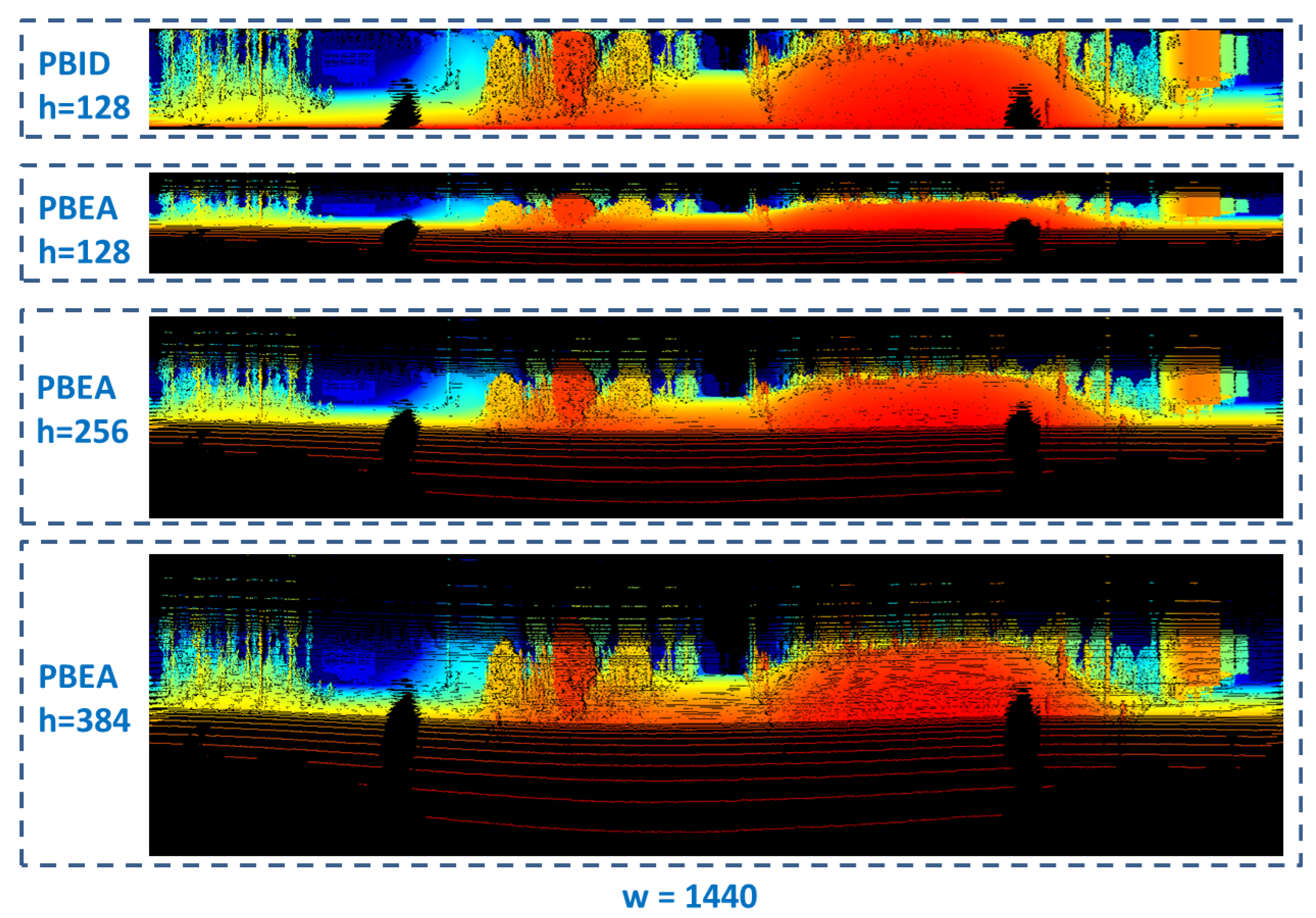
We also perform experiments on the data collected by Pandar128 LiDAR. Experiments were performed on a frame collected in urban environment when the vehicle’s speed is around 20 km/h. To compensate the LiDAR’s egomotion, the intra-frame rectification approach proposed in [18] is used. The range images generated for this LiDAR under different range image width and height are shown in Figure 9. The quantization error is shown in Figure 10.
From the error plot of Figure 10, it is observed that the error of PBID-128 is much smaller than PBEA-128, or even smaller than PBEA-256. We attribute this to two reasons: First, the vertical angular range of Pandar128 is 10 degrees larger than that of Velodyne HDL64, which makes PBEA’s equally angular partition approach prone to produce larger quantization errors. Secondly, the angular distribution of this LiDAR is not uniform, which makes it have variable angular resolution. It is calculated that the lowest angular resolution is 0.47 degrees, and the highest angular resolution is 0.12 degrees. In contrast, the angular resolution of PBEA-128 and PBEA-256 are 0.32 degrees and 0.16 degrees, respectively. From Figure 10, it is also observed that the error of PBEA-384 is smaller than PBID-128 on all range image width settings, suggesting that PBEA-384 is a preferred choice if we can tolerate its three times heavier computational load.
We also tested the RS-Ruby LiDAR in an off-road scenario with uneven terrain. This LiDAR was originally designed for urban environments. Therefore, most of its laser beams are focused in the horizontal direction. A frame is selected when the LiDAR undergoes not only translational motion but also rotational motion, thus producing a more severe intra-frame distortion. The range image generated for this frame is shown in Figure 11, and Figure 12 shows the quantization error.
From Figure 12, it is observed that the approach of PBID-128 produces the largest quantization error. The reason is mainly due to the larger intra-frame distortion, which will cause the points generated by the same laser beam to not necessarily share the same elevation angle. Compared with PBID-128, the approach of PBEA-256 and PBEA-384 produce much smaller errors in all the different settings of the range image width. Therefore, these two approaches are the recommended range image generation approaches. If we have more computational resources, PBEA-384 is the more preferable choice.
5.3. Further Discussion
From above experiments, we show that by doubling or tripling the range image height (using the approach of PBEA), a much smaller quantization error can be obtained than PBID. However, as the range image height increases, there will be more empty regions in the range image. This may hinder the performance of tasks such as object detection or semantic segmentation. For these recognition-related tasks, we can still choose to use the PBID approach, but we should bear in mind that PBID may produce larger quantization error.
In reconstruction-related tasks, such as normal estimation, terrain modeling, LiDAR odometry or LiDAR-based mapping, the approach of PBEA should be the preferred choice. Since these geometry-related tasks are mainly based on arithmetic calculations, their performance is highly related to the range image quantization error.
In addition, we have noticed that there is a trend that more and more different types of LiDAR are emerging, and each new LiDAR has a specific layout of the elevation angle. If we train an object detector on one type of LiDAR, and expect the model to be applicable for another type of LiDAR, then we have to design approaches on a standard representation (PBEA) rather than a LiDAR specific representation (PBID).
6. Concluding Remarks
In this paper, we discussed two approaches for generating range image, namely the PBID (Projection By laser ID) approach and the PBEA (Projection by Elevation Angle) approach. We believe that the range image should be an intermediate lossless representation of the original point cloud. Therefore, we analyzed these two types of approaches from the perspective of quantization errors. Further analysis shows that the quantization error has two main causes: The intra-frame distortion caused by the LiDAR’s egomotion, and the width and height of the range image. The quantization errors of both approaches are evaluated for three different types of LiDAR, namely Velodyne HDL64, Hesai Pandar128, and Robosense Ruby128.
Experimental results show that by using the approach of PBEA and setting the range image height to a relatively large value, a much smaller quantization error could be obtained than PBID. If the range image height is set to 128 for Velodyne HDL64 or 384 for Pandar128 or Ruby128, the PBEA’s quantization error is always smaller than PBID. We emphasize that in recognition-related tasks, PBID might be a preferred choice due to its compactness. However, we have to bear in mind that PBID could produce a much larger quantization error. In reconstruction-related tasks, PBEA should be the preferred choice.
Author Contributions
Conceptualization, T.W. and H.F.; methodology, T.W.; software, H.F.; validation, B.L., H.X. and R.R.; formal analysis, T.W.; investigation, H.F.; resources, T.W.; data curation, H.F.; writing—original draft preparation, H.F.; writing—review and editing, B.L., H.X., R.R. and Z.T.; visualization, H.F.; All authors have read and agreed to the published version of the manuscript.
Funding
This research received no external funding.
Conflicts of Interest
The authors declare no conflict of interest.
References
- Greenspan, M.; Yurick, M. Approximate k-d tree search for efficient ICP. In Proceedings of the Fourth International Conference on 3-D Digital Imaging and Modeling, Banff, AB, Canada, 6–10 October 2003; pp. 442–448. [Google Scholar] [CrossRef] [Green Version]
- Baur, S.A.; Moosmann, F.; Wirges, S.; Rist, C.B. Real-time 3D LiDAR flow for autonomous vehicles. In Proceedings of the IEEE Intelligent Vehicles Symposium, Paris, France, 9–12 June 2019; pp. 1288–1295. [Google Scholar] [CrossRef]
- Wang, Y.; Fathi, A.; Kundu, A.; Ross, D.A.; Pantofaru, C.; Funkhouser, T.; Solomon, J. Pillar-Based Object Detection for Autonomous Driving. arXiv 2020, arXiv:2007.10323. [Google Scholar]
- Zhou, J.; Tan, X.; Shao, Z.; Ma, L. FVNet: 3D front-view proposal generation for real-time object detection from point clouds. In Proceedings of the 12th International Congress on Image and Signal Processing, BioMedical Engineering and Informatics (CISP-BMEI), Suzhou, China, 19–21 October 2019. [Google Scholar]
- Li, B.; Zhang, T.; Xia, T. Vehicle detection from 3D lidar using fully convolutional network. arXiv 2016, arXiv:1608.07916. [Google Scholar]
- Chen, X.; Ma, H.; Wan, J.; Li, B.; Xia, T. Multi-view 3D object detection network for autonomous driving. In Proceedings of the 30th IEEE Conference on Computer Vision and Pattern Recognition, CVPR 2017, Honolulu, HI, USA, 21–26 July 2017; pp. 6526–6534. [Google Scholar]
- Meyer, G.P.; Laddha, A.; Kee, E.; Vallespi-Gonzalez, C.; Wellington, C.K. Lasernet: An efficient probabilistic 3D object detector for autonomous driving. In Proceedings of the IEEE Computer Society Conference on Computer Vision and Pattern Recognition, Long Beach, CA, USA, 16–20 June 2019; pp. 12669–12678. [Google Scholar]
- Bogoslavskyi, I.; Stachniss, C. Fast Range Image-based Segmentation of Sparse 3D Laser Scans for Online Operation. In Proceedings of the IEEE International Conference on Intelligent Robots and Systems, Daejeon, Korea, 9–14 October 2016; pp. 163–169. [Google Scholar] [CrossRef]
- Biasutti, P.; Aujol, J.F.; Brédif, M.; Bugeau, A. Range-image: Incorporating sensor topology for lidar point cloud processing. Photogramm. Eng. Remote. Sens. 2018, 84, 367–375. [Google Scholar] [CrossRef]
- Meyer, G.P.; Charland, J.; Pandey, S.; Laddha, A.; Gautam, S.; Vallespi-Gonzalez, C.; Wellington, C. LaserFlow: Efficient and Probabilistic Object Detection and Motion Forecasting. IEEE Robot. Autom. Lett. 2020. [Google Scholar] [CrossRef]
- Behley, J.; Stachniss, C. Efficient Surfel-Based SLAM using 3D Laser Range Data in Urban Environments. In Proceedings of the Robotics: Science and Systems (RSS), Pittsburgh, PA, USA, 26–30 June 2018. [Google Scholar]
- Moosmann, F.; Stiller, C. Velodyne SLAM. In Proceedings of the 2011 IEEE Intelligent Vehicles Symposium (iv), Baden-Baden, Germany, 5–9 June 2011; pp. 393–398. [Google Scholar] [CrossRef]
- Velas, M.; Spanel, M.; Hradis, M.; Herout, A. CNN for IMU assisted odometry estimation using velodyne LiDAR. In Proceedings of the 18th IEEE International Conference on Autonomous Robot Systems and Competitions, Torres Vedras, Portugal, 25–27 April 2018; pp. 71–77. [Google Scholar] [CrossRef] [Green Version]
- Cho, Y.; Kim, G.; Kim, A. Unsupervised Geometry-Aware Deep LiDAR Odometry. In Proceedings of the 2020 IEEE International Conference on Robotics and Automation (ICRA), Xi’an, China, 30 May–5 June 2020. [Google Scholar]
- Triess, L.T.; Peter, D.; Rist, C.B.; Marius Zöllner, J. Scan-based Semantic Segmentation of LiDAR Point Clouds: An Experimental Study. In Proceedings of the 2020 IEEE Intelligent Vehicles Symposium, Las Vegas, NV, USA, 19 October–13 November 2020. [Google Scholar]
- Geiger, A.; Lenz, P.; Urtasun, R. Are we ready for autonomous driving? the KITTI vision benchmark suite. In Proceedings of the 2012 IEEE Conference on Computer Vision and Pattern Recognition, Providence, RI, USA, 16–21 June 2012; pp. 3354–3361. [Google Scholar] [CrossRef]
- Carballo, A.; Lambert, J.; Monrroy, A.; Wong, D.; Narksri, P.; Kitsukawa, Y.; Takeuchi, E.; Kato, S.; Takeda, K. LIBRE: The multiple 3D LiDAR dataset. In Proceedings of the 2020 IEEE Intelligent Vehicles Symposium (IV), Las Vegas, NV, USA, 19 October–13 November 2020. [Google Scholar]
- Xue, H.; Fu, H.; Dai, B. IMU-aided high-frequency lidar odometry for autonomous driving. Appl. Sci. 2019, 9, 1506. [Google Scholar] [CrossRef] [Green Version]
- Fu, H.; Xue, H.; Ren, R. Fast Implementation of 3D Occupancy Grid for Autonomous Driving. In Proceedings of the 2020 12th International Conference on Intelligent Human-Machine Systems and Cybernetics, Hangzhou, China, 22–23 August 2020; Volume 2, pp. 217–220. [Google Scholar] [CrossRef]
- Behley, J.; Garbade, M.; Milioto, A.; Behnke, S.; Stachniss, C.; Gall, J.; Quenzel, J. SemanticKITTI: A dataset for semantic scene understanding of LiDAR sequences. In Proceedings of the IEEE/CVF International Conference on Computer Vision, Seoul, Korea, 27–28 October 2019. [Google Scholar]
- Uhrig, J.; Schneider, N.; Schneider, L.; Franke, U.; Brox, T.; Geiger, A. Sparsity invariant CNNs. In Proceedings of the 2017 International Conference on 3D Vision (3DV), Qingdao, China, 10–12 October 2017. [Google Scholar]
- Zhao, Y.; Bai, L.; Zhang, Z.; Huang, X. A Surface Geometry Model for LiDAR Depth Completion. IEEE Robot. Autom. Lett. 2021, 6, 4457–4464. [Google Scholar] [CrossRef]
- Shan, T.; Wang, J.; Chen, F.; Szenher, P.; Englot, B. Simulation-based lidar super-resolution for ground vehicles. Robot. Auton. Syst. 2020, 134, 103647. [Google Scholar] [CrossRef]
- Kusenbach, M.; Luettel, T.; Wuensche, H.J. Enhanced Temporal Data Organization for LiDAR Data in Autonomous Driving Environments. In Proceedings of the 2019 IEEE Intelligent Transportation Systems Conference, Auckland, NZ, USA, 27–30 October 2019; pp. 2701–2706. [Google Scholar] [CrossRef]
Figure 1.
Different types of LiDAR have different settings for elevation angles. Therefore, the range images generated by PBID and PBEA may be significantly different. This figure shows three types of LiDAR and the range images they generate. From left to right: The LiDAR itself; the elevation angle for each laser beam; the 3D point cloud generated by the LiDAR; range image generated by the approach of PBID (top) and PBEA (bottom).

Figure 2.
A LiDAR frame in the KITTI odometry dataset. The point cloud is colored by the laser ID. An obvious intra-frame distortion could be observed in the region outlined by the white rectangle.
Figure 2.
A LiDAR frame in the KITTI odometry dataset. The point cloud is colored by the laser ID. An obvious intra-frame distortion could be observed in the region outlined by the white rectangle.

Figure 3.
Range images generated by PBID and PBEA with varying heights for the Velodyne HDL64 LiDAR.
Figure 3.
Range images generated by PBID and PBEA with varying heights for the Velodyne HDL64 LiDAR.

Figure 4.
Quantization error under different settings of range image width and height. For PBID, the range image height has to be set to the number of LiDAR channels, i.e., 64 for the Velodyne HDL64. For PBEA, the range image height can be set to different values. The image on the left is the result of frame 700 when the LiDAR is stationary, and the image on the right is the result of frame 789 when the LiDAR is moving.

Figure 5.
The left figure shows the original point cloud, and the right figure shows the recovered point cloud after the PBID projection. As highlighted in the yellow rectangle region, the planar ground surface in the original point cloud becomes no longer flat after the PBID projection. Points are colored by height.

Figure 6.
The left figure shows the original point cloud, and the right figure shows the recovered point cloud after the PBEA projection. As highlighted in the yellow rectangle region, the continuous line segments become no longer continuous after the PBEA projection.
Figure 6.
The left figure shows the original point cloud, and the right figure shows the recovered point cloud after the PBEA projection. As highlighted in the yellow rectangle region, the continuous line segments become no longer continuous after the PBEA projection.

Figure 7.
The horizontal axis represents the area of the range image, which is calculated by multiplying the range image height by the range image width. The vertical axis is the quantization error. The left figure is the result of frame 700 in KITTI odometry sequence 07 dataset, and the right figure is the result of frame 789.

Figure 8.
Quantization error for the whole KITTI sequence 07 dataset. In the left figure, the range image width is set to 1080, whilst it is set to 2160 on the right.
Figure 8.
Quantization error for the whole KITTI sequence 07 dataset. In the left figure, the range image width is set to 1080, whilst it is set to 2160 on the right.

Figure 9.
Range images generated by PBID and PBEA with varying heights for Pandar128 LiDAR.

Figure 10.
Quantization error for Pandar128 under different settings of range image width and height.
Figure 10.
Quantization error for Pandar128 under different settings of range image width and height.

Figure 11.
Range images generated by PBID and PBEA with varying heights for the Ruby128 LiDAR.

Figure 12.
Quantization error for Ruby128.

Publisher’s Note: MDPI stays neutral with regard to jurisdictional claims in published maps and institutional affiliations. |
© 2021 by the authors. Licensee MDPI, Basel, Switzerland. This article is an open access article distributed under the terms and conditions of the Creative Commons Attribution (CC BY) license (https://creativecommons.org/licenses/by/4.0/).
Share and Cite
MDPI and ACS Style
Wu, T.; Fu, H.; Liu, B.; Xue, H.; Ren, R.; Tu, Z. Detailed Analysis on Generating the Range Image for LiDAR Point Cloud Processing. Electronics 2021, 10, 1224. https://doi.org/10.3390/electronics10111224
AMA Style
Wu T, Fu H, Liu B, Xue H, Ren R, Tu Z. Detailed Analysis on Generating the Range Image for LiDAR Point Cloud Processing. Electronics. 2021; 10(11):1224. https://doi.org/10.3390/electronics10111224
Chicago/Turabian StyleWu, Tao, Hao Fu, Bokai Liu, Hanzhang Xue, Ruike Ren, and Zhiming Tu. 2021. "Detailed Analysis on Generating the Range Image for LiDAR Point Cloud Processing" Electronics 10, no. 11: 1224. https://doi.org/10.3390/electronics10111224
Note that from the first issue of 2016, this journal uses article numbers instead of page numbers. See further details here.