Article

Optimal Placement of Reclosers in a Radial Distribution System for Reliability Improvement

1
Department of Electrical Engineering, ZHCET, Aligarh Muslim University, Aligarh 202002, India
2
Department of Industrial Engineering, College of Engineering, King Saud University, P.O. Box 800, Riyadh 11421, Saudi Arabia
3
Queensland Micro and Nanotechnology Centre, Griffith University, Nathan 4111, Australia
*
Authors to whom correspondence should be addressed.
Electronics 2021, 10(24), 3182; https://doi.org/10.3390/electronics10243182
Submission received: 18 November 2021 / Revised: 10 December 2021 / Accepted: 13 December 2021 / Published: 20 December 2021

Abstract

:
There is a need for the optimal positioning of protective devices to maximize customers satisfaction per their demands. Such arrangement advances the distribution system reliability to maximum achievable. Thus, radial distribution system (RDS) reliability can be improved by placing reclosers at suitable feeder sections. This article presents comprehensive details of an attempt to determine the reclosers’ optimal location in an RDS to maximize the utility profit by reliability improvement. Assessment of different reliability indices such as SAIDI, SAIFI, CAIFI, CAIDI, etc., with recloser placement, exhibits a considerable improvement in these indices in contrast with the absence of recloser. Consequently, a new bidirectional formulation has been proposed for the optimized arrangement of reclosers’. This formulation efficiently handles the bidirectional power flow, resulting from distributed generation (DG) unit (s) in the system. The proposed model has been solved for a test system by utilizing the Genetic algorithm (GA) optimization method. Later, test results conclude that reclosers’ optimal placement contributes significantly towards utility profit with minimum investment and outage costs.

1. Introduction

Electrical energy is a significant attribute in measuring the development index of a nation. Therefore electric utilities are introducing new techniques to enhance the efficiency and reliability of power systems [1]. Generally, the distribution side of the power system is affected by the majority of the faults. These faults (permanent or temporary) lead to sustained and momentary interruptions to the customers. High interruption in power supply causes substantial economic loss to the electric utility. These interruptions on distribution systems are mainly due to bad weather conditions, old equipment, lightning, birds, human mistakes, etc. Thus, modern distribution systems ensure the reliable transmission of high-quality power to customers. In the distribution system, the duration and frequency of the faults could be minimized by placing protective equipment such as fuses, switches, reclosers, fault indicators, etc., in various feeder sections. So, the organized positioning of these protective devices increases the system reliability at the cost of increased investment [2].
Power supply with high reliability indicates the availability of electricity to the consumers with fewer interruptions. Thus, reliability is widely described as the ability of a system to function well under the working states during its lifetime. Various reliability indices [3] such as System Average Interruption Duration Index (SAIDI), System Average Interruption Frequency Index (SAIFI), Customer Average Interruption Frequency Index (CAIFI), Average Service Availability Index (ASAI), Average energy not supplied (AENS), Customer Average Interruption Duration Index (CAIDI), Average Service Unavailability Index (ASUI), etc. aids in measuring the reliability of any power system.
A protective device present in a distribution system isolates the system’s faulty part, thereby saving the upstream system sections from interruptions [4]. However, the downstream segment connected customers experience sustained interruption till the fault is repaired. If any alternate supply is available, the downstream healthy feeder sections can be energized by disconnecting the faulty feeder section from downstream too. This enhances the system’s overall reliability by reducing the outage duration of downstream healthy feeder sections [5]. The alternate supply can be achieved from distributed generation (DG) sources which nowadays are integrated into modern distribution systems [6]. Hence, DG needs to function in islanding operation mode. For this, the DG capacity should sufficiently exceed the total load of the island [7]. The DG units presence in the distribution system forestalls the unidirectional power flow [8]. Demand-side management, grid flexibility, and security are other essential issues in a DG-enhanced distribution system [9]. The bidirectional flow of power makes the placement of protective devices even more complex as a feeder section may be fed from upstream or downstream [10]. Therefore, the conventional optimal placement strategies are needed to be upgraded [11].
So far, lots of research has been done, focusing on the optimal positioning of the protective equipments in a distribution system. The early research work that contributed to the optimal positioning of the protective equipment in a RDS is suggested in references [12,13,14,15]. A procedure for the optimal arrangement of sectionalizing switches by considering the maintenance costs, system outage, and investment costs have been advised in [12]. Furthermore, simulated annealing (SA) algorithm has been utilized to resolve this problem. Furthermore, the simulated annealing (SA) technique has been utilized to resolve this issue. In [13], alternative power supply source potential to adjoining feeders has been suggested for the optimal positioning of the switches in an RDS. Direct search algorithm has been recommended for optimal positioning of switch in [14] An automatic calculation procedure has been presented in [15], which determines the optimum location and total count of automatic sectionalizing switching equipment. The authors of the article referenced [16] proposed a new model for analyzing the impact of the islanded operation of a DG-enhanced distribution system. Additionally, this article presents testing of the new model by determining the compromise done between the reliability and operational cost for the 135-bus system. A new algorithm has been proposed in [17] that enhances the reliability attribute of an RDS by utilizing the concept of the best arrangement of protective devices. In [18], a new approach considering the optimal placement of remote control switches in a DG-enhanced RDS has been suggested, which considers reliability, equipment cost, and DG unavailability. The authors in [19] have proposed two different models for enhancing the reliability of a RDS with DG. The first model is employed in optimal positioning of reclosers in the RDS, while the second model is utilized for operating DG in islanded mode. For evaluating the impact of long-term load shedding on reliability indices of a DG enhanced RDS, a new algorithm has been proposed in [20]. For this, an advance under frequency load shedding scheme has been used to improve the success rate of the islanding process. In [21], a general novel concept is presented for the best positioning of switching equipments in an RDS. However, this formulation cannot handle the bidirectional power flow as it is applicable for the systems without DG units.
The above studies have significantly contributed towards protective devices optimal placement in a RDS. However, the assumption to place the DG units at the feeder end in a DG-enhanced RDS may not be a practical approach. Hence, there is a need to develop a new model which is capable of dealing with the situations when DG units are located at any bus (not only the terminal bus). This article presents a novel model which is specifically designed for the optimal placement of reclosers in a DG enhanced RDS. The summary of the main contributions of the paper is listed in the following points:
1.
An analytical model has been devised to deal with the optimal position issues of reclosers in several zones/islands of a radial distribution system, including DG(s).
2.
The proposed framework is capable of handling the location(s) of DG(s) connected at any node(s) (not necessarily at the end node) of the distribution framework.
The article is configured into the following segments: Section 2 accounts for the genetic algorithm methodology. The calculation procedure to determine the reliability of an islanded portion of a distribution system with reclosers is comprehensively discussed in Section 3. Section 4 demonstrates the discussion on the formulated problem. The outcomes of the proposed work are explained in Section 5. Lastly, Section 6 puts forth the paper conclusion.

2. Genetic Algorithm

Genetic Algorithm (GA) is inspired by the evolutionary attribute, predominantly, natural selection process. Biologically motivated attributes, mutation, crossover, and selection are the main components of GA strategy. GA techniques are widely employed in the optimization and search process [22]. GA generates the candidate solutions population in optimization problems, which evolves over the iterations to give the best output. Generally, binary digits 0 and 1 are utilized for encoding solutions. However, other array type combinations can be used. The candidate solutions can be mutated and altered to evolve, and thus each has specific properties (i.e., in the form of genotype or chromosomes). The basic flowchart of the GA technique is exhibited in Figure 1.
Initially, a population is randomly generated, and the evolution process occurs in each iteration. The population per the iteration count is known as a generation. The objective function is computed for each generation, and later, the best solution is chosen from the current population. Then, the selected individuals are modified to produce a new generation. This iterative process is continued until the optimum solution is achieved for the population. The two main constituents of the GA are:
1.
Solution domain representation in genetic form.
2.
Evaluation of the solutions per the objective function.
After defining the genetic representation and objective function, GA implantation requires the following steps:
1.
Initialization: A population constituting of N individuals (in binary form) having definite length, i.e., bit number S, is generated. A binary matrix mathematically represents the population. The individual count in the population is signified by the number of rows in the binary matrix, while the count of its column represents the individual decision length.
2.
Assessment: This evaluation process helps in the individual selection process. The selection is made per the objective function (F) values. Then, the selected individuals are employed to generate a new generation.
3.
Genetic Operation: The following tasks are the basis of GA strategy.
(a)
Selection: The probability (P r ) of selecting the rth individual is calculated per the roulette wheel selection, as depicted in Equation (1).
P r = F r n = 1 n = N F n
(b)
Crossover: This operation executes the reproduction process by crossing the selected individual pairs to generate children (i.e., novel ones).
(c)
Mutation: In this process, one or more chromosome genes are altered, resulting in a change in random bits.
(d)
Insertion: The worst solutions are replaced in this step. The decision is made after comparing the population-produced integration of the previous and new generations.
4.
End: This process brings forths the best individuals for a new population. The whole course of action is iterative and stops when desired results are achieved.

3. Recloser Placement in a Radial Distribution System to Improve the Reliability of the System

A recloser is a circuit breaker equipped with an automatic mechanism that can auto reclose its contact after it has been opened because of a fault. The failure rate of a recloser depends on its age and maintenance [23]. It is mostly used in overhead distribution systems for detecting and interrupting faults. As the majority of faults are in distribution systems, therefore the use of reclosers can remarkably enhance the reliability of these systems. Most of the recent reclosers are controlled by electronic relays, which give a great deal of flexibility in protection, restoration, and communication [12].
Autoreclosers use either vacuum, oil, or sulphur hexafluoride as arc quenching medium. The ratings of reclosers vary from 2.4 kV to 38 kV for system voltage, from 10 A to 1200 A for load current and from 1 kA to 16 kA for fault current. As per recloser standards, the number of recloser attempts is limited to four. The fundamental responsibility of a recloser is to quickly detect the fault cases and provide a successful response based on the type of fault. This can be done by a probabilistic approach together with the detection of the fault category. If a recloser is placed at a specific feeder section, then it will prevent interruption of all loads upstream of that feeder section. This results in a significant decrease in the failure rates of the upstream loads, which reduces the various reliability indices, namely system average interruption frequency index (SAIFI), energy not supplied (ENS), etc.
The power flow in the distribution system becomes non-unidirectional when the DG unit is present in the system. This leads to the increment in the complexities of the problems relating to the reclosers optimal position in a distribution system. To understand it better, consider an islanded portion of a RDS shown in Figure 2. The island consists of 13 buses, 12 feeder segments, and 13 load points. Also, an alternate supply is connected at node 7, and node 1 is attached to a DG. The DG in the system is competent enough to provide supply for all the loads linked with all the 13 load points. Moreover, when external fault circumstances occur in the island, a recloser is placed at the alternate supply point, which detaches the island from the alternate supply.
The island shown in Figure 2 is to be protected by reclosers for enhancement of reliability. An assumption is made regarding the recloser placement in any feeder segment that it can be arranged at the start of any feeder segment (seen from the side of DG). One clear example is when the fault occurs within the island, i.e., fault in any of the feeder segments, then reclosers located at the two sources (i.e., alternate supply and DG) performed the tripping action to isolate the island from the supplies [11]. When the fault is cleared, by removing the faulty feeder segment with the help of protective equipments which are already deployed at the several sections of the feeder in the island, alternate supply or DG energizes the healthy feeder segments per the need. Let X R , k be the binary variables representing a recloser in kth feeder section. Furthermore, consider
X R , k = 0 , if a recloser is connected in k t h feeder segment 1 , otherwise

3.1. Evaluation of λ i , j

The parameter λ i , j signifies the jth load failure rate per the fault in the ith feeder segment and, mathematically computed as,
λ i , j = b i b c ( i , j ) × λ i × ( k ϵ D F d ( i , j ) X R , k ) + ( 1 b i b c ( i , j ) ) × λ i × ( k ϵ F d ( i , j ) X R , k ) ( k ϵ D F d ( i , j ) X R , k )
b i b c ( i , j ) = 1 , if the j t h load is located downstream of the i t h feeder segment as seen from the side of the DG 0 , otherwise
Hence, the system [BIBC] matrix is illustrated in Figure 1 can be computed as per Equation (5).
B I B C = L 1   L 2   L 3     L 4     L 5     L 6     L 7     L 8   L 9     L 10   L 11   L 12   L 13 F 1 F 2 F 3 F 4 F 5 F 6 F 7 F 8 F 9 F 10 F 11 F 12    0       1       1       1       1       1       1       1       1       1       1       1       1       0       0       1       1       1       1       1       1       1       1       1       1       1       0       0       0       1       1       1       1       0       0       0       0       1       1       0       0       0       0       1       1       1       0       0       0       0       1       1       0       0       0       0       0       1       1       0       0       0       0       0       0       0       0       0       0       0       0       1       0       0       0       0       0       0       0       0       0       0       0       0       0       1       1       1       1       0       0       0       0       0       0       0       0       0       0       1       1       1       0       0       0       0       0       0       0       0       0       0       0       1       1       0       0       0       0       0       0       0       0       0       0       0       0       1       0       0       0       0       0       0       0       0       0       0       0       0       0       1       1       0       0       0       0       0       0       0       0       0       0       0       0       1   
Feeder segment fault leads to the failure of a load point, whose failure rate depends on its position with regards to the location of the feeder segment. The load point can present either in the upstream or downstream direction concerning the feeder segment.

3.1.1. Downstream Load concerning the Faulted Feeder

Suppose λ 3 , 13 needs to be computed, which corresponds to the load failure load L 13 arising because of the fault in the feeder section; F 3 , then Equation (5) is utilized to know the value of b i b c ( 3 , 13 ) . The b i b c ( 3 , 13 ) is 1, since the load L 13 lies in the downstream directions of the feeder segment F 3 , as seen from the DG side.
Afterwards, the value of b i b c ( 3 , 13 ) is substituted in Equation (3) to calculate λ 3 , 13 , as follows,
λ 3 , 13 = λ 3 × ( k ϵ D F d ( 3 , 13 ) X R , k )
Thus, feeder segments set between the end node of the feeder section F 3 and alternate supply node, i.e., D F S e c ( S n , 3 ) , can be evaluated as:
DF Sec ( S n , 3 ) = { F 4 , F 5 , F 6 }
Likewise, feeder segments set between the 13th node and feeder section end node F 3 can be computed using the following equation:
DF Sec ( 13 , 3 ) = { F 4 , F 11 , F 12 }
Therefore, feeder sections common to DF Sec ( S n , 3 ) and DF Sec ( 13 , 3 ) , i.e., DFd ( 3 , 13 ) can be mathematically computed as,
DFd ( 3 , 13 ) = DF Sec ( S n , 3 ) DF Sec ( 13 , 3 ) = { F 4 }
From Equations (6) and (7), it can be observed that λ 3 , 13 = 0, when recloser is incorporated into the feeder section F 4 scientifically when X R , 4 = 0. This suggests that the fault that occurred in F 3 feeder segment can be cleared by placing a recloser in F 4 feeder segment, and thus, supply to the L 13 load can be recommenced by utilizing the alternate supply. So, when the recloser device is absent in the F 4 feeder section (i.e., λ 3 , 13 = λ 3 ), supply to the load L 13 can be only be continued after repairing the fault at the feeder F 3 .

3.1.2. Upstream Load with Reference to Faulty Feeder Segment

Let the L 4 load failure rate due to the faulty condition in the feeder segment F 12 , i.e., λ 12 , 4 , requires to be evaluated. For this case, per the Equation (5), b i b c ( 12 , 4 ) = 0 as the L 4 load is located on the upstream side of the F 12 feeder segment as seen from the side of DG.
Therefore, λ 12 , 4 can be computed per the Equation (8).
λ 12 , 4 = λ 12 × ( k ϵ F d ( 12 , 4 ) X R , k ) ( k ϵ D F d ( 12 , 4 ) X R , k )
Furthermore,
F S e c ( 1 , 12 ) = { F 1 , F 2 , F 3 , F 4 , F 11 , F 12 }
F S e c ( 4 , 12 ) = { F 4 , F 11 , F 12 }
Hence,
F d ( 12 , 4 ) = F S e c ( 1 , 12 ) F S e c ( 4 , 12 ) = { F 4 , F 11 , F 12 }
The feeder segments set between the end node of the feeder section F 12 and alternate supply node, i.e., D F S e c ( S n , 12 ) , can be evaluated as:
DF Sec ( S n , 12 ) = { F 5 , F 6 , F 11 , F 12 }
Likewise, feeder segments set between the 4th node and the feeder section F 12 end node can be computed using the following equation:
DF Sec ( 4 , 12 ) = { F 4 , F 11 , F 12 }
Therefore, feeder sections common to both DF Sec ( S n , 12 ) and DF Sec ( 4 , 12 ) , i.e., DFd ( 12 , 4 ) can be mathematically evaluated as,
DFd ( 12 , 4 ) = DF Sec ( S n , 12 ) DF Sec ( 4 , 12 ) = { F 11 , F 12 }
Equations (8)–(10) imply that reclosers placement in any of the feeder sections F 4 , F 11 , or F 12 clears the fault in the feeder segment F 12 , which further allows the supply continuation to the load L 4 through the DG source. The presence of reclosers in any of the feeder sections F 4 , F 11 , or F 12 makes the parameter, λ 12 , 4 = 0 in contrast, reclosers absence leads to λ 12 , 4 = λ 12 . The absence of reclosers demands the fast repairing of the F 12 faulted feeder to maintain the supply to the L 4 load.

3.2. Estimation of the Parameter r i , j

The jth load outage time under the fault in the ith feeder segment is represented by the parameter r i , j , which can be modeled by using Equation (11).
r i , j = b i b c ( i , j ) × { r i ( k ϵ D F d ( i , j ) X R , k ) + ( 1 b i b c ( i , j ) ) × { r i ( k ϵ F d ( i , j ) X R , k ) ( k ϵ D F d ( i , j ) X R , k )
Now, the outage time for the load L 12 which takes place as a effect of the fault in the F 3 feeder section; indicated by r 3 , 12 . So, to evaluate r 3 , 12 , Equation (5) is employed to determine the b i b c ( 3 , 12 ) , which is equals to 1 since the load L 12 as seen from the DG side located in downstream of the F 3 feeder segment. Hence, r 3 , 12 is determines per the following equation:
After substituting the value of b i b c ( 3 , 12 ) in Equation (11), r 3 , 12 can be written as,
r 3 , 12 = r 3 × ( k ϵ D F d ( 3 , 12 ) X R , k )
Further,
D F S e c ( S n , 3 ) = { F 4 , F 5 , F 6 }
D F S e c ( 12 , 3 ) = { F 4 , F 11 }
Therefore,
D F d ( 3 , 12 ) = D F S e c ( S n , 3 ) D F S e c ( 12 , 3 ) = { F 4 }
From Equations (12) and (13), it can be implied that recloser presence in the feeder segment here F 4 helps in maintain the supply to the load (here L 12 ) by clearing the fault in the feeder section F 3 . In this case, r 3 , 12 = 0. However, when the recloser is not included in the F 4 feeder section, then r 3 , 12 = r 3 .
Thus, TIC and ENS can be computed by utilizing Equations (14) and (15), respectively.
T I C = j = 1 n l i = 1 n b r λ i , j × I C P i , j × L j
E N S = j = 1 n l i = 1 n b r λ i , j × r i , j × L j k W h r / y e a r

4. Problem Formulation

A bi-directional analytical model has been presented in this paper to provide a solution for the optimal positioning of reclosers in DG enhanced radial distribution network problems. This model increases the utility profit by improving the reliability of the system. Additionally, this framework reduces the investment and outage cost of the system.

4.1. Objective Function

The objective function is modeled per the following equations for reclosers’ optimal positioning in an RDS with a DG system.
M a x i m i z e f = [ ( ( Revenue earned as a result of reduction in TIC ) + Revenue earned as a result of reduction in ENS ) ( Reclosers installation and maintenance cost ) ] = { j = 1 n l i = 1 n b r ( λ i λ i , j ) I C P T i , j ) L j } F a c 1 + { j = 1 n l i = 1 n b r ( λ i r i λ i , j r i , j ) L j } × C E × F a c 2 { ( i = 1 n b r ( 1 X R , i ) ) C R } ( 1 + C m 100 F a c 3 )
where,
F a c 1 = 1 a 1 N s 1 a 1 , a 1 = ( 1 + L c 100 ) ( 1 + i c 100 ) ( 1 + i r 100 )
F a c 2 = 1 a 2 N s 1 a 2 , a 2 = ( 1 + L c 100 ) ( 1 + r E 100 ) ( 1 + i r 100 )
F a c 3 = 1 a 3 N s 1 a 3 , a 3 = ( 1 + r m 100 ) ( 1 + i r 100 )
The values of the parameters ‘ λ i , j ’ and ‘ r i , j ’ used in Equations (16) are calculated using Equations (3) and (11), respectively. The first term of Equation (16) represents the NPW of the revenue collected because of the reduction in customer interruption cost. From [4], several customer interruption costs are taken for the computation. The second term in Equation (16) stands for the NPW of the revenue collected from the extra supply of energy (resulting from the reduced ENSs) to the consumers for the interval of N s years. The values of interruption costs for various customers are taken from [4]. Equation (16) the third term denotes the NPW of the reclosers maintenance and installation cost for a period of N s years.

4.2. Constraints

The constraints imposed on the objective function (as expressed by Equation (16) are as follows:
1.
On the same feeder section, at most, one recloser can be placed.
2.
The total count of the reclosers which are deployed in the distribution network must lie within the limits per the utility specifications. This restraint is modeled per the inequality constraint shown in Equation (17).
i = 1 n b r ( 1 X R , i ) N R

5. Case Study

5.1. Manual Placement of a Recloser

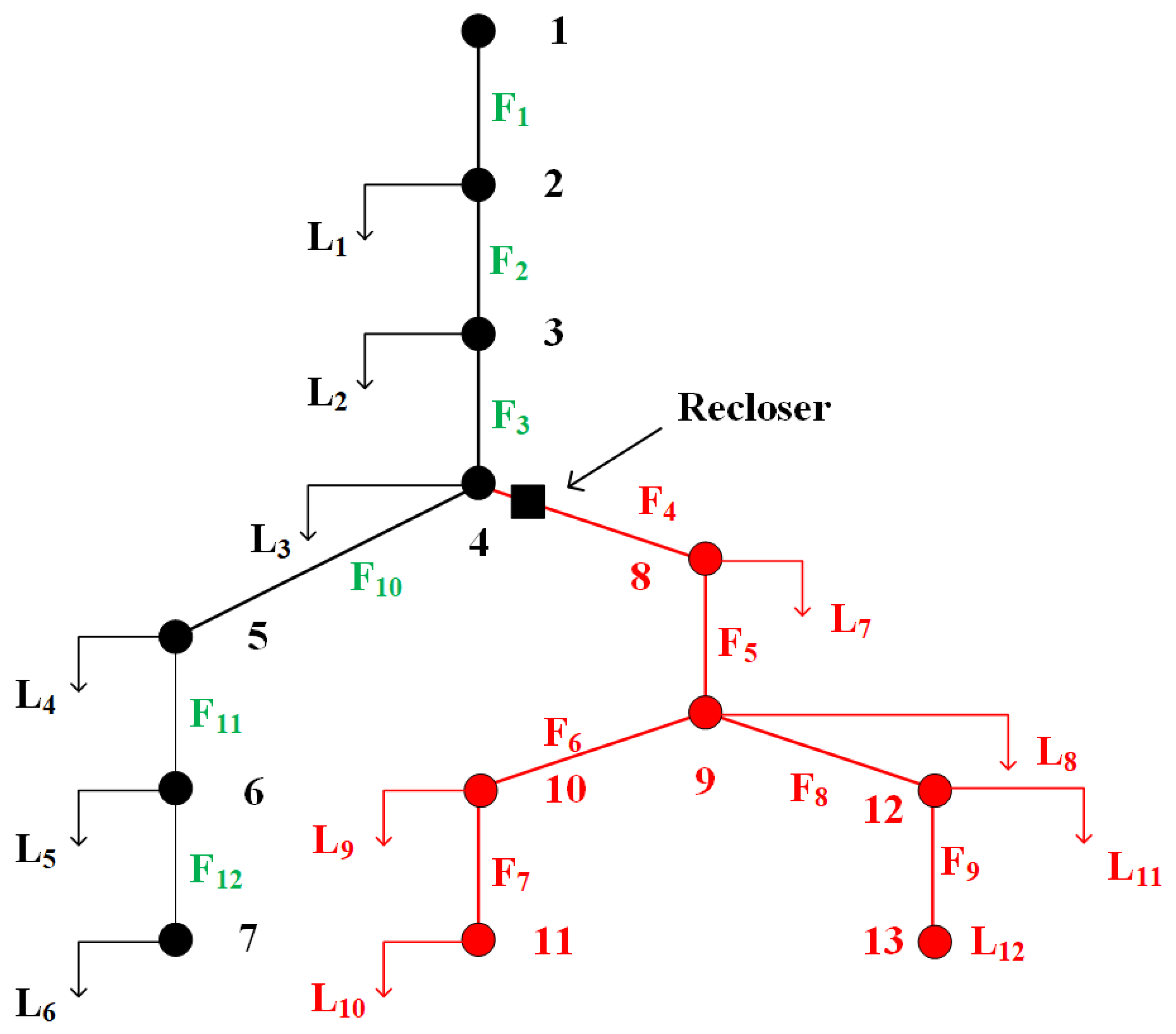
Figure 3 depicts a system consisting of 13-bus RDS, having 12 load points and 12 feeder sections. The data for this system have been taken from the article referenced as [4]. Table 1 shows various reliability indices [3] for the base case (without placing any recloser) for this system.
A recloser present in a feeder section reduces sustained interruptions of all the loads upstream of the feeder segment for any downstream fault as per the referenced feeder. However, downstream loads of the feeder (having recloser) experience sustained interruption because of the fault in any of the downstream feeder segments concerning the referenced feeder (usually faulted feeder). Hence, to analyze such an effect, a recloser is deployed at the beginning of each feeder section of the 13-bus RDS, one by one. For each of these cases, the various reliability indices are listed in Table 2. From this table, it can be clearly implied that placing a recloser in F 1 feeder section outcomes that none of the loads can be saved for any fault in the system. Hence, no improvement is seen in the reliability indices compared to the base case (i.e., Table 1). This shows that the recloser placement in the feeder section F 1 will incur additional operation and maintenance costs without any benefit. However, the placement of the recloser in other feeder sections has significantly improved the reliability indices of the system. Though these indices ( SAIFI , SAIDI , CAIDI , etc.) quantify the reliability for a RDS, there is still a need to formulate an exhaustive objective function for planning this perspective [6].
Thus, the utility profit results from the placement of a recloser in an RDS, which may be written as follows [1]:
P r o f i t = [ ( Revenue earned because of reduction in TIC ) + ( Revenue earned as a result of reduction in ENS ) ( Installation and maintenance cost of a recloser ) ]
For each of the above cases, the utility profit (per Equation (18)), when reclosers are placed one by one in different feeder sections of the 13-bus RDS is shown in Table 3. From this table, the following conclusion can be made that when the recloser is placed at feeder section F 1 , the utility’s profit is negative, which is evident as there is a requirement for additional maintenance and installation cost without any profit as discussed above. It can further be inferred that the maximum gain of Rs. 17,089,522.31 can be achieved when the recloser is placed at feeder section F 4 . When the recloser is placed in feeder section F 4 , all the loads downstream of F 4 (highlighted in red color in Figure 4) cannot be saved when a fault occurs in any downstream feeders. However, for all these faults, loads that lie upstream of F 4 will remain uninterrupted. For this case, the modified failure rate of the various feeder segments of 13-bus RDS is shown in Table 4. The above benefit of recloser placement may be maximized by finding optimal count and positions of the reclosers to be placed in the system. This has been discussed in the next part of this section.

5.2. Optimal Placement of Reclosers

DGs increased penetration in distribution systems prohibits unidirectional power flow. This makes the optimal placement problem of reclosers more complex. Hence, to check the effectiveness of the suggested model, a more extensive test system with multiple DG units has been chosen for the optimal placement of reclosers. A 69-bus RDS having total reactive and active loads of 2.69 MVAr and 3.80 MW, respectively, is illustrated in Figure 5 [24]. System bus and line data are considered from [25]. For the considered scenario, the system failure data are given in Table 5. Moreover, data related to other costs are taken from Table 5. By employing the strategy suggested in [24], the optimal sizes and locations of 3 D G s ( D G 1 , D G 2 , and D G 3 at 0.85 lagging power factor) in 69-bus RDS have been determined as 0.4769 MW, 0.3124 MW, and 1.4552 MW at buses 11, 21 and 61, respectively, which helps in improving the system voltage profile and minimizing the power loss.
In the case of DGs presence, the formation of zones or islands for each DG is a first step towards deploying reclosers in the system. The region surrounding a DG is known as a zone or island, which is competent enough to provide supply to all the system connected loads alone by ensuring power (active and reactive) balance and security constraints (i.e., frequency and voltage control). It has been assumed that utility efficiently controls the security constraints and power balance in the system.
The result for load flow of 69-bus RDS as shown in Figure 5 is depicted in Table 6, which considers the DG generations and the average values of loads. This table clearly describes power flow directions in several feeder segments. The DGs presence in the system makes the power flow negative, which is shown by boldface font, representing the reverse/upstream power flow, in Table 6.
The power flow directions analysis in several feeder segments and the total count of loads which surrounds the D G 1 concludes that D G 1 can easily handle the supply to all the loads located at buses 10, 11, 12, 13, 14, 15, 16, 66, 67, 68, and 69, hence leading to the formation of ‘Zone 1’ as depicted in Figure 5. In the same way, D G 2 is also sufficient to supply all the loads connected to buses 17, 18, 19, 20, 21, 22, 23, 24, 25, 26, and 27, which results in ‘Zone 2’ formation. Furthermore, it should be taken into account D G 3 has low capacity, because of which it cannot form any zone. Apart from that, ‘Zone 0’ considers the remaining loads (which are outside of Zone 1 and Zone 2) and can only be supplied by D G 3 and the substation. Generally, reclosers are arranged during the time of installation of the devices in the system, which segregates any two zones and is named zone reclosers. This type of reclosers immediately isolates the healthy zones in the system from the faulty zone when a condition of fault arises in any part of the zones and disconnects the faulty system DG. Afterward, the faulty zone DG working in the islanding mode provides supply to faulty zone remaining healthy feeder segments [26].
After the zone formation, the optimal positioning of reclosers in each zone is done by evaluating the objective function (Equation (16)) using the GA optimization technique [27] in the MATLAB environment. The results of the optimized placement of reclosers in the 69-bus system exhibited in Figure 5 zones are arranged in Table 7. This table suggests that in Zone 0, the optimal positions of reclosers are in feeder sections F4, F27, F35, and F46. In Zone 1 and Zone 2, no recloser can be deployed optimally. This happens as the utility’s profit from allocating a recloser in these zones is lesser than the expenditure results from recloser(s) installation and maintenance for customer types (commercial, residential, industrial) and the given loads of the zones. The protected zones cost (i.e., interruption and outage costs) for Zone 0, Zone 1, and Zone 2 are Rs. 7,469,685.04, Rs. 621,861.78 and Rs. 410,044.53, respectively. Hence, the systems’ total cost, including protected zones (total costs of three protected zones) is Rs. 8,501,591.35. The original unprotected 69-bus system, as depicted in Figure 5 cost is Rs. 27,026,816.41, and the price of two-zone reclosers placed at feeder segments F9 and F17 of the 69-bus system illustrated in Figure 4 is Rs. 900,000. Table 8 constitutes the various cost components associated with the 69-bus system shown in Figure 5. The data in the table signifies that the total utility profit for reclosers optimal allocation in three zones of the 69-bus system illustrated in Figure 5 is observed as Rs. 17,625,225.06.
For the purpose of comparison, the formulated problem has also been solved with DE and MINLP optimization techniques used in [4]. As the objective function is highly non-convex in nature, each technique has been run 100 times to evaluate the profits’ standard deviation. The obtained results have been shown in Table 9. Following observation from the table can be made that all these methods are capable of reaching the best function value (total profit). However, in terms of accuracy (minimum standard deviation), GA has outperformed among the three methods.

6. Conclusions

This article demonstrates a new formulation for reclosers’ optimal allocation in a DG-enhanced RDS. The effect on the reliability of an RDS is analyzed by manual as well as the optimal placements of reclosers. The proposed formulation can handle bidirectional power flow due to the integration of DG units in an RDS. Using the GA optimization technique, this problem has been solved for a 69-bus RDS. The test system different zones have been made for DG units operating successfully in islanding mode. Furthermore, mean values of DG generations and loads are utilized to determine the zone boundaries. The test results analysis sums up that deploying the protective equipment at the optimal positions in different test system zones significantly increases the utility’s profit. Moreover, when a faulty condition arises in any system part, such arrangements of reclosers also promote the DG units of each zone to operate in islanding mode. Hence, DG helps in providing the supply to the loads located on the island. This work can further be extended by considering the uncertainties in loads and DG generations.

Author Contributions

Conceptualization, A.A. and M.T.; Formal analysis, A.A., M.T., M.Z., P.V., M.A., S.A., A.S. and M.A.H.; Investigation, A.A., M.T., M.Z., P.V. and A.S.; Methodology, A.A., M.T., M.Z., P.V. and A.S.; Funding Acquisition, M.A. and S.A.; Writing—original draft, A.A. and M.T.; Writing—review & editing, M.Z., P.V., M.A., S.A., A.S. and M.A.H. All authors have read and agreed to the published version of the manuscript.

Funding

The authors extend their appreciation to King Saud University for funding this work through Researchers Supporting Project number (RSP-2021/313), King Saud University, Riyadh, Saudi Arabia.

Acknowledgments

The authors acknowledge King Saud University for funding this work through Researchers Supporting Project number (RSP-2021/313), King Saud University, Riyadh, Saudi Arabia.

Conflicts of Interest

The authors declare no conflict of interest.

References

  1. Sultan, H.; Ansari, S.J.; Alam, A.; Khan, S.; Sarwar, M.; Zaid, M. Reliability improvement of a radial distribution system with recloser placement. In Proceedings of the 2019 International Conference on Computing, Power and Communication Technologies (GUCON), New Delhi, India, 28–29 September 2019; pp. 736–741. [Google Scholar]
  2. Alam, A.; Pant, V.; Das, B. Optimal placement of protective devices and switches in a radial distribution system with distributed generation. IET Gener. Transm. Distrib. 2020, 14, 4847–4858. [Google Scholar] [CrossRef]
  3. Okorie, P.; Aliyu, U.; Jimoh, B.; Sani, S. Reliability indices of electric distribution network system assessment. J. Electron. Commun. Eng. Res. 2015, 3, 1–6. [Google Scholar]
  4. Alam, A.; Pant, V.; Das, B. Switch and recloser placement in distribution system considering uncertainties in loads, failure rates and repair rates. Electr. Power Syst. Res. 2016, 140, 619–630. [Google Scholar] [CrossRef]
  5. Popovic, Z.; Knezevic, S.; Brbaklic, B. Optimal number, type and location of automation devices in distribution networks with distributed generation. In Proceedings of the CIRED Workshop 2016, Helsinki, Finland, 14–15 June 2016; pp. 1–4. [Google Scholar]
  6. Mitra, J.; Vallem, M.R.; Singh, C. Optimal deployment of distributed generation using a reliability criterion. IEEE Trans. Ind. Appl. 2016, 52, 1989–1997. [Google Scholar] [CrossRef]
  7. Heidari, A.; Agelidis, V.; Kia, M. Considerations of sectionalizing switches in distribution networks with distributed generation. IEEE Trans. Power Deliv. 2015, 30, 1401–1409. [Google Scholar] [CrossRef]
  8. Holguin, J.P.; Rodriguez, D.C.; Ramos, G. Reverse power flow (rpf) detection and impact on protection coordination of distribution systems. IEEE Trans. Ind. Appl. 2020, 56, 2393–2401. [Google Scholar] [CrossRef]
  9. Wu, Y.; Tan, W.; Huang, S.; Chiang, Y.; Chiu, C.; Su, C. Impact of generation flexibility on the operating costs of the taiwan power system under a high penetration of renewable power. IEEE Trans. Ind. Appl. 2020, 56, 2348–2359. [Google Scholar] [CrossRef]
  10. Constante-Flores, G.E.; Illindala, M.S. Data-driven probabilistic power flow analysis for a distribution system with renewable energy sources using monte carlo simulation. IEEE Trans. Ind. 2019, 55, 174–181. [Google Scholar] [CrossRef]
  11. Wang, L.; Singh, C. Reliability-constrained optimum placement of reclosers and distributed generators in distribution networks using an ant colony system algorithm. IEEE Trans. Syst. Man Cybern. Part C (Appl. Rev.) 2008, 38, 757–764. [Google Scholar] [CrossRef]
  12. Levitin, G.; Mazal-Tov, S.; Elmakis, D. Genetic algorithm for optimal sectionalizing in radial distribution systems with alternative supply. Electr. Power Syst. Res. 1995, 35, 149–155. [Google Scholar] [CrossRef]
  13. Billinton, R.; Jonnavithula, S. Optimal switching device placement in radial distribution systems. Power Deliv. IEEE Trans. 1996, 11, 1646–1651. [Google Scholar] [CrossRef]
  14. Wang, P.; Billinton, R. Demand-side optimal selection of switching devices in radial distribution system planning. IEE Proc.—Gener. Transm. Distrib. 1998, 145, 409–414. [Google Scholar] [CrossRef]
  15. Celli, G.; Pilo, F. Optimal sectionalizing switches allocation in distribution networks. IEEE Trans. Power Deliv. 1999, 14, 1167–1172. [Google Scholar] [CrossRef]
  16. Meneses, C.A.P.; Mantovani, J.R.S. Improving the grid operation and reliability cost of distribution systems with dispersed generation. IEEE Trans. Power Syst. 2013, 28, 2485–2496. [Google Scholar] [CrossRef]
  17. Ray, S.; Bhattacharya, A.; Bhattacharjee, S. Optimal placement of switches in a radial distribution network for reliability improvement. Int. J. Electr. Power Energy Syst. 2016, 76, 53–68. [Google Scholar] [CrossRef]
  18. Pombo, A.V.; Murta-Pina, J.; Pires, V.F. A multiobjective placement of switching devices in distribution networks incorporating distributed energy resources. Electr. Power Syst. Res. 2016, 130, 34–45. [Google Scholar] [CrossRef]
  19. Velasquez, M.A.; Quijano, N.; Cadena, A.I. Optimal placement of switches on DG enhanced feeders with short circuit constraints. Electr. Power Syst. Res. 2016, 141, 221–232. [Google Scholar] [CrossRef]
  20. Issicaba, D.; da Rosa, M.A.; Resende, F.O.; Santos, B.; Lopes, J.A.P. Long-term impact evaluation of advanced under frequency load shedding schemes on distribution systems with DG islanded operation. IEEE Trans. Smart Grid 2019, 10, 238–247. [Google Scholar] [CrossRef]
  21. Alam, A.; Alam, M.N.; Pant, V.; Das, B. Placement of protective devices in distribution system considering uncertainties in loads, temporary and permanent failure rates and repair rates. IET Gener. Distrib. 2018, 12, 1474–1485. [Google Scholar] [CrossRef]
  22. Issaadi, W.; Mazouzi, M.; Issaadi, S. Command of a Photovoltaic System by Artificial Intelligence, Comparative Studies with Conventional Controls: Results, Improvements, and Perspectives. In Proceedings of the 8th Proceedings of International Conference on Modelling, Identification and Control (ICMIC), Algiers, Algeria, 15–17 November 2017; pp. 583–591. [Google Scholar]
  23. Thompson, C.C.; Barriga, C.I. Relationship between historicaltrends, equipment age, maintenance, and circuit breaker failure rates. IEEE Trans. Ind. Appl. 2019, 55, 5699–5707. [Google Scholar] [CrossRef]
  24. Nekooei, K.; Farsangi, M.M.; Nezamabadi-Pour, H.; Lee, K.Y. An improved multi-objective harmony search for optimal placement of DGs in distribution systems. IEEE Trans. Smart Grid 2013, 4, 557–567. [Google Scholar] [CrossRef]
  25. Chakravorty, M.; Das, D. Voltage stability analysis of radial distribution networks. Int. J. Electr. Power Energy Syst. 2001, 23, 129–135. [Google Scholar] [CrossRef]
  26. Heidari, A.; Agelidis, V.G.; Kia, M.; Pou, J.; Aghaei, J.; Shafie-Khah, M.; Catalo, J.P.S. Reliability optimization of automated distribution networks with probability customer interruption cost model in the presence of DG units. IEEE Trans. Smart Grid 2017, 8, 305–315. [Google Scholar] [CrossRef]
  27. Rezaei, N.; Uddin, M.N.; Amin, I.K.; Othman, M.L.; Marsadek, M. Genetic algorithm-based optimization of overcurrent relay coordination for improved protection of dfig operated wind farms. IEEE Trans. Ind. Appl. 2019, 55, 5727–5736. [Google Scholar] [CrossRef]
Figure 1. Flowchart depicting the GA algorithm strategy.
Electronics 10 03182 g001
Figure 2. An islanded portion of a RDS having 13 buses, and 13 load points.
Electronics 10 03182 g002
Figure 3. 13-bus RDS [1].
Electronics 10 03182 g003
Figure 4. A recloser placed in feeder section F 4 of the 13-bus RDS.
Electronics 10 03182 g004
Figure 5. Zonesformation of 69-bus RDS per the average values of load and DG generations.
Electronics 10 03182 g005
Table 1. Reliability indices of 13-bus system before placement of any recloser.
Reliability IndicesValues
SAIFI1.9000
SAIDI7.2000
CAIDI3.7895
ASUI0.00082
ASAI0.9992
AENS76.0533
Table 2. Reliability indices of the 13-bus system with a recloser placement in different feeder sections.
Feeder Section/Indices SAIFI SAIDI CAIDI ASUI ASAI AENS
F 1 1.90007.20003.78950.000820.999276.0533
F 2 1.83336.94813.78950.000790.999254.0667
F 3 1.71676.52783.80260.000750.999348.9180
F 4 1.47785.60003.78950.000640.999448.0800
F 5 1.48525.51113.71070.000630.999448.915
F 6 1.73706.71113.86350.000770.999270.0911
F 7 1.81116.84443.77910.000780.999272.0163
F 8 1.61485.61113.47480.000640.999456.0117
F 9 1.72966.17783.57170.000710.999363.5644
F 10 1.51116.22784.12130.000710.999365.3913
F 11 1.68706.77414.01540.000770.999271.3978
F 12 1.80377.00743.88500.000800.999274.0348
Table 3. Profit after a recloser placement in various feeder sections of the 13-bus RDS.
Feeder SectionProfit (Rs.)
F 1 −691,041.30
F 2 13,701,517.83
F 3 17,081,996.51
F 4 17,089,522.31
F 5 16,708,017.16
F 6 3,009,722.43
F 7 1,775,248.20
F 8 11,781,879.09
F 9 7,116,814.51
F 10 5,757,516.55
F 11 2,151,941.38
F 12 546,014.03
Table 4. Failure rate of various feeder sections after placement of a recloser in feeder section F 4 .
Feeder Section/Load L 1 L 2 L 3 L 4 L 5 L 6 L 7 L 8 L 9 L 10 L 11 L 12
F 1 0.10.10.10.10.10.10.10.10.10.10.10.1
F 2 0.150.150.150.150.150.150.150.150.150.150.150.15
F 3 0.20.20.20.20.20.20.20.20.20.20.20.2
F 4 0000000.250.250.250.250.250.25
F 5 0000000.150.150.150.150.150.15
F 6 0000000.10.10.10.10.10.1
F 7 0000000.10.10.10.10.10.1
F 8 0000000.150.150.150.150.150.15
F 9 0000000.20.20.20.20.20.2
F 10 0.250.250.250.250.250.250.250.250.250.250.250.25
F 11 0.150.150.150.150.150.150.150.150.150.150.150.15
F 12 0.10.10.10.10.10.10.10.10.10.10.10.1
λ L 0.950.950.950.950.950.951.91.91.91.91.91.9
Table 5. Data for system failure of the 69-bus test system.
Feeder λ rFeeder λ rFeeder λ rFeeder λ r
Section(f/yr)(hrs)Section(f/yr)(hrs)Section(f/yr)(hrs)Section(f/yr)(hrs)
F10.14F180.12F350.152F520.14
F20.155F190.14F360.12F530.155
F30.26F200.155F370.14F540.26
F40.253F210.26F380.155F550.253
F50.152F220.253F390.26F560.152
F60.12F230.152F400.253F570.12
F70.14F240.12F410.152F580.152
F80.155F250.14F420.12F590.12
F90.26F260.155F430.14F600.253
F100.253F270.26F440.155F610.152
F110.152F280.253F450.26F620.12
F120.12F290.152F460.253F630.14
F130.14F300.12F470.152F640.155
F140.155F310.14F480.12F650.26
F150.26F320.155F490.253F660.253
F160.253F330.26F500.152F670.152
F170.152F340.253F510.12F680.12
Table 6. Power flow of 69-bus RDS per the average values of loads and DG generations.
FeederPower FlowFeederPower FlowFeederPower Flow
Segment(MW)Segment(MW)Segment(MW)
F11.630215809F240.028799061F470.850849442
F21.630215809F250.028799061F480.771784167
F31.352907876F260.014399698F490.38594987
F40.502058434F270.091542298F500.044747552
F50.502058434F280.065541009F510.003654441
F60.499439308F290.039538701F520.319511669
F70.458495629F300.039538701F530.315081684
F80.337638207F310.039538701F540.288161683
F9−0.012343989F320.039538701F550.26361675
F10−0.040844349F330.025528836F560.26361675
F110.25618987F340.006007105F570.26361675
F120.050820447F350.185765635F580.26361675
F130.042636159F360.159764251F590.158537031
F140.034437679F370.133760476F600.158537031
F150.034437679F380.133760476F610.337492105
F16−0.012259186F390.109752994F620.303601763
F17−0.073773655F400.085745469F630.303601763
F18−0.135288277F410.084544474F640.062657794
F19−0.135288277F420.084544474F650.036686906
F20−0.13631386F430.078537641F660.018343461
F210.063031846F440.078537641F670.057232044
F220.057589592F450.039268827F680.02861604
F230.057589592F460.850849442
Table 7. Optimized placement of reclosers in three islands/zones of 69-bus RDS illustrated in Figure 5.
ZonesLocation ofCost of Protected
ReclosersZone (Rs.)
Zone 0F4 F27 F35 F467,469,685.04
Zone 1Nil621,861.78
Zone 2Nil410,044.53
System (including protected zones) total cost (in Rs.) = 8,501,591.35
Table 8. Cost components associated with the optimal placement of reclosers in three zones of the 69-bus RDS exhibited in Figure 5.
1. Price for the original unprotected system devoid of zoning (Rs.)27,026,816.41
2. Price for the system (including protected zones) in (Rs.)8,501,591.35
3. 2 zone reclosers cost in (Rs.)900,000.00
4. Overall profit in Rs. (1-2-3)17,625,225.06
Table 9. Comparison of results with different methods.
MethodsBest ProfitStandard Deviation
(Rs.)(% of Mean)
GA17,625,225.060.09
DE17,625,225.060.17
MINLP17,625,225.060.14
Publisher’s Note: MDPI stays neutral with regard to jurisdictional claims in published maps and institutional affiliations.

