
Facial Emotion Recognition Using Transfer Learning in the Deep CNN
by
 , , and
M. A. H. Akhand
1,* ,
,
Shuvendu Roy
1,
Nazmul Siddique
2,
Md Abdus Samad Kamal
3,* and
Tetsuya Shimamura
4 1
Department of Computer Science and Engineering, Khulna University of Engineering & Technology, Khulna 9203, Bangladesh
2
School of Computing, Engineering and Intelligent Systems, Ulster University, Londonderry BT48 7JL, UK
3
Graduate School of Science and Technology, Gunma University, Kiryu 376-8515, Japan
4
Graduate School of Science and Engineering, Saitama University, Saitama 338-8570, Japan
*
Authors to whom correspondence should be addressed.
Electronics 2021, 10(9), 1036; https://doi.org/10.3390/electronics10091036
Submission received: 3 March 2021
/
Revised: 12 April 2021
/
Accepted: 24 April 2021
/
Published: 27 April 2021
(This article belongs to the Special Issue Deep Learning Technologies for Machine Vision and Audition)
Abstract
:Human facial emotion recognition (FER) has attracted the attention of the research community for its promising applications. Mapping different facial expressions to the respective emotional states are the main task in FER. The classical FER consists of two major steps: feature extraction and emotion recognition. Currently, the Deep Neural Networks, especially the Convolutional Neural Network (CNN), is widely used in FER by virtue of its inherent feature extraction mechanism from images. Several works have been reported on CNN with only a few layers to resolve FER problems. However, standard shallow CNNs with straightforward learning schemes have limited feature extraction capability to capture emotion information from high-resolution images. A notable drawback of the most existing methods is that they consider only the frontal images (i.e., ignore profile views for convenience), although the profile views taken from different angles are important for a practical FER system. For developing a highly accurate FER system, this study proposes a very Deep CNN (DCNN) modeling through Transfer Learning (TL) technique where a pre-trained DCNN model is adopted by replacing its dense upper layer(s) compatible with FER, and the model is fine-tuned with facial emotion data. A novel pipeline strategy is introduced, where the training of the dense layer(s) is followed by tuning each of the pre-trained DCNN blocks successively that has led to gradual improvement of the accuracy of FER to a higher level. The proposed FER system is verified on eight different pre-trained DCNN models (VGG-16, VGG-19, ResNet-18, ResNet-34, ResNet-50, ResNet-152, Inception-v3 and DenseNet-161) and well-known KDEF and JAFFE facial image datasets. FER is very challenging even for frontal views alone. FER on the KDEF dataset poses further challenges due to the diversity of images with different profile views together with frontal views. The proposed method achieved remarkable accuracy on both datasets with pre-trained models. On a 10-fold cross-validation way, the best achieved FER accuracies with DenseNet-161 on test sets of KDEF and JAFFE are 96.51% and 99.52%, respectively. The evaluation results reveal the superiority of the proposed FER system over the existing ones regarding emotion detection accuracy. Moreover, the achieved performance on the KDEF dataset with profile views is promising as it clearly demonstrates the required proficiency for real-life applications.
1. Introduction
Emotions are fundamental features of humans that play important roles in social communication [1,2]. Humans express emotion in different ways, such as facial expression [3,4], speech [5], body language [6]. Among the elements related to emotion recognition, facial expression analysis is the most popular and well-researched area. Ekman and Friesen [7], and Ekman [8] have performed extensive research in human facial expressions and identified universal facial expressions: happiness, sadness, anger, fear, surprise, disgust, and neutral states. Recently, recognizing emotion from facial expressions has become an appealing research topic in psychology, psychiatry, and mental health [9]. Automated detection of emotions from facial expressions is also essential for smart living [10], health care systems [11], emotion disorder diagnosis in autism spectrum disorder [12], schizophrenia [13], human-computer interaction (HCI) [14], human-robot interaction (HRI) [15] and HRI based social welfare schemes [16]. Therefore, facial emotion recognition (FER) has attracted the attention of the research community for its promising multifaceted applications.
Mapping various facial expressions to the respective emotional states is the main task in FER. The classical FER consists of two main steps: feature extraction and emotion recognition. In addition, image preprocessing, including face detection, cropping, resizing, and normalization, is also necessary. Face detection removes background and non-face areas and then crops the face area. Feature extraction from the processed image is the most important task in a classical FER system, and the existing methods use distinguished techniques such as discrete wavelet transform (DWT), linear discriminant analysis, etc. [17,18]. Finally, the extracted features are used to understand emotions by classifying them, usually using the neural network (NN) and other different machine learning techniques.
Currently, Deep NNs (DNNs), especially convolutional neural networks (CNNs), have drawn attention in FER by virtue of its inbuilt feature extraction mechanism from images [19,20]. A few works have been reported with the CNN to solve FER problems [21,22,23,24,25,26]. However, the existing FER methods considered the CNN with only a few layers, although its deeper model is shown to be better at other image-processing tasks [27]. The facts behind this may be the challenges related to FER. Firstly, recognition of emotion requires a moderately high-resolution image, meaning to work out high dimension data. Secondly, the difference in faces due to different emotional states is very low, which eventually complicates the classification task. On the other hand, a very deep CNN comprises a huge number of hidden convolutional layers. Training a huge number of hidden layers in the CNN becomes cumbersome and does not generalize well. Moreover, simply increasing the number of layers does not increase the accuracy after a certain level due to the vanishing gradient problem [28]. Various modifications and techniques are introduced to the deep CNN architecture and the training technique to increase accuracy [29,30,31,32]. The widely used pre-trained DCNN models are VGG-16 [29], Resnet-50, Resnet-152 [33], Inception-v3 [31] and DenseNet-161 [34]. But training such a deep model requires a lot of data and high computational power.
An appropriate FER system might be capable of recognizing emotion from different facial angle views. In many real-life situations, the target person’s frontal views may not always be captured perfectly. The best-suited FER system should be capable of recognizing emotion from profile views taken at various angles, although such recognition is challenging. It is to be noted that most of the existing methods considered frontal images only, and some studies used the dataset with profile views but excluded the profile view images in the experiment for convenience [17,35,36]. Therefore, it is necessary for a more practical FER system that is capable of recognizing emotion from both the frontal and profile views.
This study proposes a FER system comprising DCNN and transfer learning (TL) to reduce development efforts. The TL technique is a popular method of building models in a timesaving way where learning starts from patterns that have already been learned [37,38,39]. The repurposing of pre-trained models avoids training from the sketch that requires a lot of data and leverages the huge computational efforts. In other words, TL reuses the knowledge through pre-trained models [40] that have been trained on a large benchmark dataset for a similar kind of problem. The motivations behind the study are: low-level basic features are common for most images, and an already trained model should be useful for classification by only fine-tuning the high-level features. In the proposed FER system, a pre-trained DCNN (e.g., VGG-16), originally modeled for image classification, is adopted by replacing its upper layers with the dense layer(s) to make it compatible with FER. Next, with facial emotion data, the model is fine-tuned using the pipeline strategy, where the dense layers are tuned first, followed by tuning of each DCNN block successively. Such fine-tuning gradually improves the accuracy of FER to a high level without the need to model a DCNN from scratch with random weights. The emotion recognition accuracy of the proposed FER system is tested on eight different pre-trained DCNN models (VGG-16, VGG-19, ResNet-18, ResNet-34, ResNet-50, ResNet-152, Inception-v3, and DenseNet-161) and well-known KDEF and JAFFE facial image datasets. FER on the KDEF dataset is more challenging due to the diversity in images with different profile views along with frontal views, and most of the existing studies considered a selected set of frontal views only. The proposed method is found to show remarkable accuracy on both datasets with any pre-trained model. The evaluation results reveal the superiority of the proposed FER system over the existing ones in terms of emotion detection accuracy. Moreover, the achieved performance on the KDEF dataset with profile views is promising as it clearly meets the proficiency required for real-life industry applications.
The main contributions of this study can be summarized as follows.
- (i)
- Development of an efficient FER method using DCNN models handling the challenges through TL.
- (ii)
- Introduction of a pipeline training strategy for gradual fine-tuning of the model up to high recognition accuracy.
- (iii)
- Investigation of the model with eight popular pre-trained DCNN models on benchmark facial images with the frontal view and profile view (where only one eye, ear, and one side of the face is visible).
- (iv)
- Comparison of the emotion recognition accuracy of the proposed method with the existing methods and explore the proficiency of the method, especially with profile views that is important for practical use.
The rest of the paper is organized as follows: Section 2 briefly reviews the existing FER methods. Section 3 gives a brief overview of CNN, DCNN models, and TL for a better understanding of the proposed FER. Section 4 explains the proposed TL-based FER. Section 5 presents experimental studies. Section 6 gives an overall discussion on model significance, outcomes on benchmark datasets and related issues. Section 7 concludes the paper with a discussion on future research directions.
2. Related Works
Several techniques have been investigated for FER in the last few decades. The conventional pioneer methods first extract features from the facial image and then classify emotion from feature values. On the other hand, the recent deep learning-based methods perform the FER task by combining both the steps in its single composite operational process. A number of studies reviewed and compared the existing FER methods [17,18,41,42], and the recent ones among them [41,42] included the deep learning-based methods. The following subsections briefly describe the techniques employed in the prominent FER methods.
2.1. Machine Learning-Based FER Approaches
Automatic FER is a challenging task in the artificial intelligence (AI) domain, especially in its machine learning subdomain. Different traditional machine learning methods (e.g., K-nearest neighbor, neural network) are employed through the evolution of the FER task. The pioneering FER method by Xiao-Xu and Wei [43] added wavelet energy feature (WEF) to the facial image first, then used Fisher’s linear discriminants (FLD) to extract features and finally classify emotion by using K-nearest neighbor (KNN) method. KNN was also used for classification in FER by Zhao et al. [44], but they used principal component analysis (PCA) and non-negative matrix factorization (NMF) for feature extraction. Feng et al. [45] extracted local binary pattern (LBP) histograms from different small regions of the image, combined those into a single feature histogram, and finally, used a linear programming (LP) technique to classify emotion. Zhi and Ruan [46] derived facial feature vectors from 2D discriminant locality preserving projections. Lee et al. [47] extended wavelet transform for 2D, called contourlet transform (CT), for feature extraction from the image and used a boosting algorithm for classification. Chang and Huang [48] incorporated face recognition in FER for better expression recognition of individuals, and they used radial basis function (RBF) neural network for classification.
A number of methods used the support vector machine (SVM) to classify emotion from extracted feature values using distinct techniques. In this category, Shih et al. [49] investigated various feature representations (e.g., DWT, PCA); and DWT with 2D-linear discriminant analysis (LDA) is shown to outperform others. Shan et al. [50] evaluated different facial representations based on local statistical features and LBPs with different variants of SVM in their comprehensive study. Jabid et al. [51] investigated an appearance-based technique called local directional pattern (LDP) for feature extraction. Recently, Alshami et al. [35] investigated two feature descriptors called facial landmarks descriptor and center of gravity descriptor with SVM. The comparative study of Liew and Yairi [17] considered SVM and several other methods (e.g., KNN, LDA) for classification on feature extracted employing different methods, including Gabor, Haar, and LBP. The most recent study by Joseph and Geetha [52] investigated different classification methods, which are logistic regression, LDA, KNN, classification and regression trees, naive Bayes, and SVM on their proposed facial geometry-based feature extraction. The major limitation of the aforementioned conventional methods is that they only considered frontal views for FER as features from frontal and profile views are different through traditional feature extraction methods.
2.2. Deep Learning-Based FER Approaches
The deep learning approach for FER is a relatively new approach in machine learning, and hitherto several CNN-based studies have been reported in the literature. Zhao and Zhang [22] integrated a deep belief network (DBN) with the NN for FER, where the DBN is used for unsupervised feature learning, and the NN is used for the classification of emotion features. Pranav et al. [26] considered a standard CNN architecture with two convolutional-pooling layers for FER on self-collected facial emotional images. Mollahosseini et al. [21] investigated a larger architecture adding four inception layers with two convolutional-pooling layers. Pons and Masip [53] formed an ensemble of 72 CNNs, where individual CNNs were trained with different sizes of filters in convolutional layers or the different number of neurons in fully connected layers. Wen et al. [54] also considered the ensemble of CNNs, but they trained 100 CNNs, and the final model was with a selected number of CNNs. Ruiz-Garcia et al. [36] initialized weights of CNN with encoder weights of stacked convolutional auto-encoder and trained with facial images. Such CNN initialization is shown to outperform CNN with random initialization. Ding et al. [55] extended deep face recognition architecture to the FER and proposed an architecture called FaceNet2ExpNet. Further, FaceNet2ExpNet is extended by Li et al. [23] using transfer learning. Jain et al. [56] considered hybrid architecture of deep learning with CNN and recurrent neural network (RNN) for FER. A hybrid architecture with TL has been investigated by Shaees et al. [57], where features from pre-trained AlexNet are classified using SVM. Recently, Bendjillali et al. [24] used CNN to FER from DWT extracted features. Liliana [58] employed a relatively deep CNN architecture with 18 convolutional layers, with four subsampling layers for FER. Most recently, Shi et al. [59] considered a clustering approach with CNN for FER. Ngoc et al. [25] investigated a graph-based CNN for FER from landmark features of faces. Jin et al. [60] considered unlabeled data along with labeled data in their CNN-based method. On the other hand, Porcu et al. [61] evaluated different data augmentation techniques, including synthetic images to train the deep CNN, and a combination of synthetic images with other methods performed better for FER. The existing deep learning-based methods have also considered the frontal images, and most of the studies even excluded the profile view images of the dataset in the experiment to make the task easy [17,35,36,61].
3. Overview of CNN, Deep CNN Models and Transfer Learning (TL)
Pre-trained DCNN models and TL technique are the basis of this study. Several pre-trained DCNN models are investigated to identify the best-suited one for FER. The following subsections present an overview of CNN, considered DCNN models, and TL motivation to make the paper self-contained.
3.1. Convolutional Neural Network (CNN)
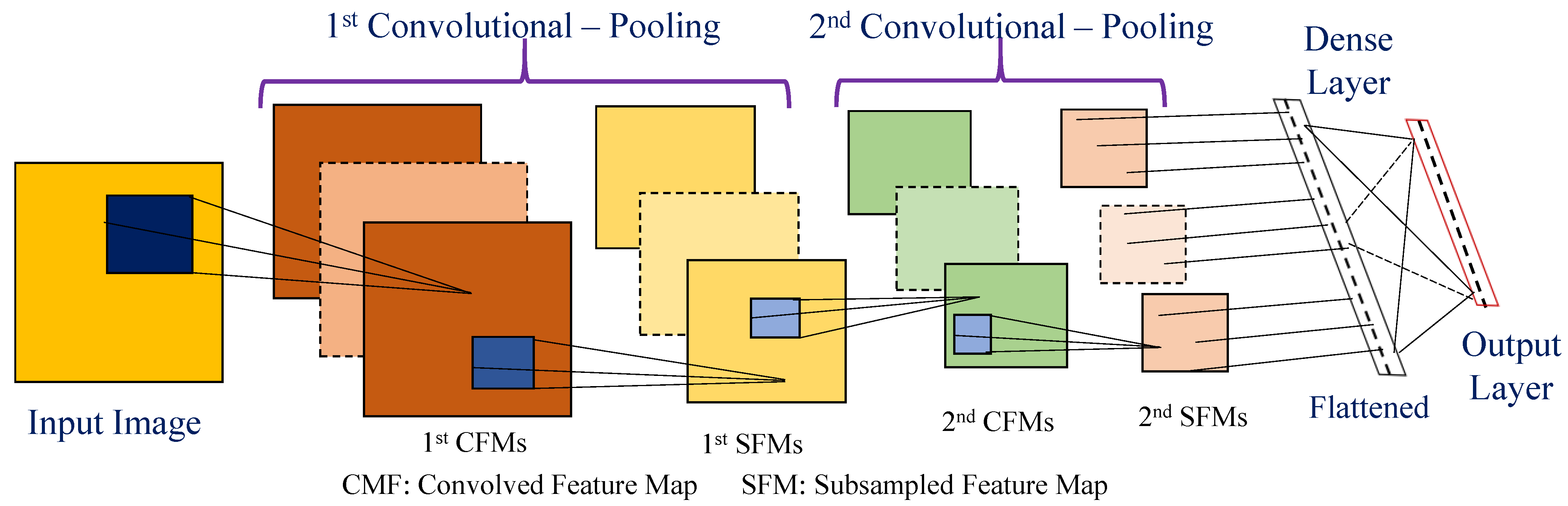
Due to the inherent structure of CNN, it is the best suitable model for the image domain [20]. A CNN consists of an input layer, multiple convolutional-pooling hidden layers, and an output layer. Basically, convolution is a mathematical operation on two functions to produce a third function expressing a modified shape of the function. The small-sized (e.g., 3 × 3, 5 × 5) kernel of a CNN slides through the image to find useful patterns in it through convolution operation. Pooling is a form of non-linear downsampling. A pooling layer combines non-overlapping areas at one layer into a single value in the next layer. Figure 1 shows the generic architecture of a standard CNN with two convolutional-pooling layers. The 1st convolution layer applies convolution operation onto the input image and generates the 1st convolved feature maps (CMFs) those are the input of successive pooling operation. The 1st pooling operation produces the 1st subsampled feature maps (SFMs). After the 1st pooling, the 2nd convolutional-pooling layer operations are performed. Flattening the 2nd SFMs’ values, the fully connected layer (i.e., dense layer) performs the final reasoning where the neurons are connected to all activations in the previous layer. The final layer, also called the loss layer, specifies how training penalizes the deviation of the actual output from the predicted output. Such a CNN architecture is popular for pattern recognition from small-sized (e.g., 48 × 48) input images such as handwritten numeral recognition, and the detailed description of CNN is available in the existing studies [19,62].
3.2. DCNN Models and TL Motivation
A DCNN has many hidden convolutional layers, and it takes high dimensional images leading to very challenging input and training. Different DCNN models hold different significant arrangements and connections in the convolutional layers [19]. The first model that obtained good accuracy on ImageNet was AlexNet [63] which uses five layers in CNN. ZFnet [64] is based on a similar idea but with fewer parameters that achieved an equivalent accuracy level. It has replaced big kernels with smaller ones. While AlexNet used 15 million images for training, ZFNet used only 1.3 million images to get a similar result. Later, VGG-16 [29] proposed a deeper model of depth 16 with 13 convolutional layers and smaller kernels [65]. VGG-19 is another model in this category with 16 convolutional layers.
An important concept employed by most of the later models is the skip-connection [33], which was introduced in residual neural network (ResNet) [33]. The basic idea of skip-connection is to direct the input of a layer and add it to the output after some layers. This provides more information to the layer and helps to overcome the vanishing gradient problem. Currently, a few different ResNet models with different depth is available, for example, ResNet-18, 34, 50 and 152 are among them; the number of convolutional layers in a model has one less layer than the depth size mentioned with the model’s name (e.g., ResNet-50 has 49 convolutional layers).
Along with a single skip connection, DenseNet [34] introduced dense skip connection among layers. This means, each layer receives signals from its previous layers, and the output of that layer is used by all the subsequent layers. The input of a single layer is combined with the channel concatenation of previous layers. Traditional CNNs with L layers have L direct connections; on the contrary, DenseNet has [L(L + 1)/2] direct connections. Since each layer has direct access to its preceding layers, there is a lower information bottleneck in the network. Thus, the model becomes much thinner and compact and yields high computational efficiency. DenseNet blocks are built up by concatenating feature maps, so the input to deeper layers will be extensively incurring massive computation for deeper layers. They use relatively cheaper convolution with size one by one to reduce the dimension of channels that also improves the parameter efficiency. Along with these, non-linearity on the kth layer is calculated by concatenating 0-(k − 1) features and using a non-linear function of this feature map. There are several versions of this model, and the DenseNet-161 contains 157 convolutional layers with four modules.
Inception [66] is another deep CNN model which is built up using several modules. The basic idea behind the inception is to try different filters and stack the modules up after adding non-linearity. This helps getting rid of picking up a fixed filter and lets the network learn whatever combinations of these filters it wants. This module uses one by one convolution to shrink the number of channels so that one can reduce the computation cost. Besides stacking these inception modules, the network has some branch layers, which also predicts the model output and gives some prior idea of whether the model is overfitting or under-fitting. There are several versions of the inception model, and the Inception-v3 contains 40 convolutional layers with several inception modules.
Training any large DCNN model is a complex task as the network has many parameters to tune. It is common that a massive network requires relatively large training data. Training with a small or insufficient amount of data might result in over-fitting. For some tasks, it is difficult to get a sufficient amount of data for proper training of the DCNN. Moreover, a huge amount of data is not readily available for some cases. However, research has shown that TL [37,38] can be very useful to solve this issue. Basically, TL is a concept to use the knowledge representation learned from the different tasks but similar applications. It is reported that the TL technique works better when both tasks are similar [37,39]. Recently, TL has been investigated on the task different from its training and is shown to achieve good results [67,68], which is the motivation behind this study.
4. Facial Emotion Recognition (FER) Using TL in Deep CNNs
FER using a pre-trained DCNN model through appropriate TL is the main contribution of this study. Mahendran and Vedaldi [69] visualized what CNN layers learn. The first layer of the CNN captures basic features like the edge and corners of an image. The next layer detects more complex features like textures or shapes, and the upper layer follows the same mechanism towards learning more complex patterns. As the basic features are similar in all images, tasks for FER in the lower layers in DCNN are identical to other image-based operations, such as classification. Since training a DCNN model from scratch (i.e., with randomly initialized weights) is a huge task, a DCNN model already trained on another task can be fine-tuned employing the TL approach for emotion recognition. A DCNN model (e.g., VGG-16) pre-trained with a large dataset (e.g., ImageNet) for image classification [29] is suitable for FER. The following subsections describe TL concepts for FER and the proposed FER method in detail with required illustrations.
Figure 2 shows the general architecture of a TL-based DCNN model for FER, where the convolutional base is a part of pre-trained DCNN excluding its own classifier, and the classifier on the base is the newly added layers for FER. As a whole, repurposing a pre-trained DCNN comprises two steps: replacement of the original classifier with a new one and fine-tune the model. The added classifier part is generally a combined dense layer(s) of those that are fully connected. From a practical point of view, both selecting a pre-trained model and determining a size-similarity matrix for fine-tuning are important in TL [40,70]. There are three widely used strategies for training the model in fine-tuning: train the entire model, train some layers leaving others frozen and train the classifier only (i.e., freeze the convolution base) [71]. In the case of a similar task, training the only classifier and/or few layers is enough in fine-tuning for learning the task. On the other hand, for dissimilar tasks, full model training is essential. Thus, fine-tuning is performed on the added classifier and a selected portion (or full) of the convolution base. A portion selection for fine-tuning and appropriate training methods for fine-tuning are tedious jobs to get better FER, which tasks are managed in this study through a pipeline strategy.
Figure 3 illustrates the proposed FER system with VGG-16, the well-known pre-trained DCNN model. The available VGG-16 model is trained with the ImageNet dataset to classify 1000 image objects. The pre-trained model is modified for emotion recognition redefining the dense layers, and then fine-tuning is performed with emotion data. In defining the architecture, the last dense layers of the pre-trained model are replaced with the new dense layer(s) to recognize a facial image into one of seven emotion classes (i.e., afraid, angry, disgusted, sad, happy, surprised, and neutral). A dense layer is a regular, fully connected, linear layer of a NN that takes some dimension as input and outputs a vector of the desired dimension. Therefore, the output layer contains only seven neurons. The fine-tuning is performed on the architecture having the convolution base of the pre-trained model plus the added dense layer(s). A cleaned emotion dataset prepared through preprocessing (i.e., resizing, cropping, and other tasks) is used to train in fine-tuning. In the case of testing, a cropped image is placed to the input of the system, and the highest output probability of emotion is considered to be the decision. VGG-16 may be replaced with any other DCNN models, e.g., ResNet, DenseNet, Inception. Therefore, the size of the proposed model depends on the size of the pre-trained model used and the architecture of the added dense layer(s).
Figure 4 shows the detailed schematic architecture of the proposed model with a detailed pre-trained VGG-16 model, plus dense layers for FER. The green section in the figure is the added portion having three fully connected layers in a cascade fashion. The first one is a ‘Flatten’ layer, which converts the metric into a one-dimensional vector; its task is the only representation and to make it compatible for emotion recognition operation in the next layers, and no operation is performed on the data. The other two layers are densely connected: the first one is a hidden layer that converts the comparatively higher-dimensional vector into an intermediate-length vector which is the input of the final layer. The final layer’s output is a vector with the size of individual emotional states.
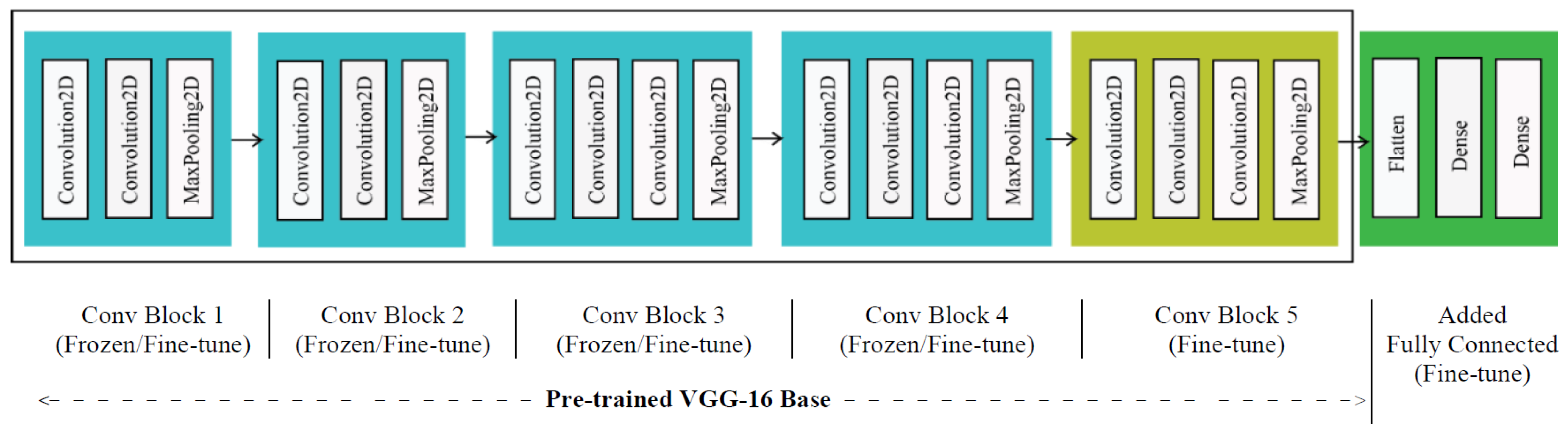
The full model in the same pipeline of pre-trained DCNN and the added dense layers give the opportunity for fine-tuning the dense layers and required few layers of the pre-trained model with emotion data. The pre-trained VGG-16 model shown in Figure 4 consists of five convolutional blocks, and each block has two or three convolutional layers and a pooling layer. The 2D convolutional and pooling operations indicate that the procedures are performed in the 2D image format. Conv Block 1 (i.e., the first block) has two convolutional layers and a MaxPooling layer in a cascade fashion. The output of the layer is the input of Conv Block 2. Suppose the first convolutional layer of Block 1 takes the inputs of size 224 × 224 × 3 for input color image size 224 × 224; after successive convolution and pooling operations in different blocks, the output size of the VGG-16 model is 7 × 7 × 512. The flatten layer converts it into a linear vector of size 25,088 (=7 × 7 × 512), which is the input to the first dense layer. It performs a linear operation and outputs a vector of 1000 length, and this is the input to the final dense layer of length 128. The output of the final dense layer is seven for seven different emotional expressions.
Fine-tuning is the most important step in the TL-based FER method, and a carefully selected technique is employed to fine-tune the proposed model owing to achieve an improved result. Added dense layer(s) always need to be fine-tuned as the weights of each layer are randomly initialized. On the other hand, a part of (or full) pre-trained model may be considered in the fine-tuning step. Conv Block 5 of VGG-16 model with ‘Fine-tune’ mark in Figure 4 indicates fine-tuning of this block is essential and fine-tuning of other four blocks is optional thus marked with ‘frozen/fine-tune’. The training process of fine-tuning is also important. If the training of both the added layers and the pre-trained model are carried out together, the random weights of dense layers will lead to a poor gradient, which will be propagated through the trained portion, causing deviation from a good result. Therefore, in fine-tuning, a pipeline strategy is employed to train the model with facial emotion dataset: added dense layers are trained first, and then the selected blocks of the pre-trained VGG-16 model are included in the training step by step. To train four different layers of Conv Block 5 of VGG-16 model, fine-tuning increases slowly instead of training all at a time. It helps diminish the effect of initial random weight and keeps track of accuracy. It is worth mentionable that the best outcome with a particular DCNN model may get different fine-tuning options for different datasets depending on the size and other features.
Adam [72] algorithm, the popular optimization algorithm in computer vision and natural language processing applications, is used in the training process of fine-tuning. Adam is derived from two optimization methods: adaptive gradient descent (AdaGrad) which maintains a different learning rate for different parameters of the model [73]; and root mean square propagation (RMSProp) [74], which also maintains different learning rate and it is the average of previous magnitudes. It has two momentum parameters beta1 and beta2, and the user-defined values of the parameters control the learning rate of the algorithm during training. A detailed description of the Adam approach is available in [72].
Image cropping and data augmentation are considered for training the proposed model. Cropped face portion from the image is considered as input in the FER task to enhance facial properties. On the other hand, data augmentation is an effective technique, especially for image data, of making new data from the available data. In this case, new data is generated by rotating, shifting, or flipping the original image. The idea is that if we rotate, shift, scale, or flip the original image, this will still be the same subject, but the image is not the same as before. The process is embedded in the data loader in training. Every time it loads the data from memory, a small transformation is applied to the image to generate slightly different data. As the exact same data is not given to the model, the model is less prone to overfittings. This is very helpful, especially when the dataset is not very large, like the case of FER. With this augmentation, the new cost function of the FER model to considering all images is:
where N represents the number of images in the dataset and T is the number for transformation to perform over an image.
5. Experimental Studies
This section investigates the efficiency of the proposed FER system using TL on DCNN on two benchmark datasets. Firstly, a description of benchmark datasets and experimental setup are presented. Finally, the outcome of the proposed model on the benchmark datasets is compared with some existing methods to verify the effectiveness of the proposed model.
5.1. Benchmark Datasets
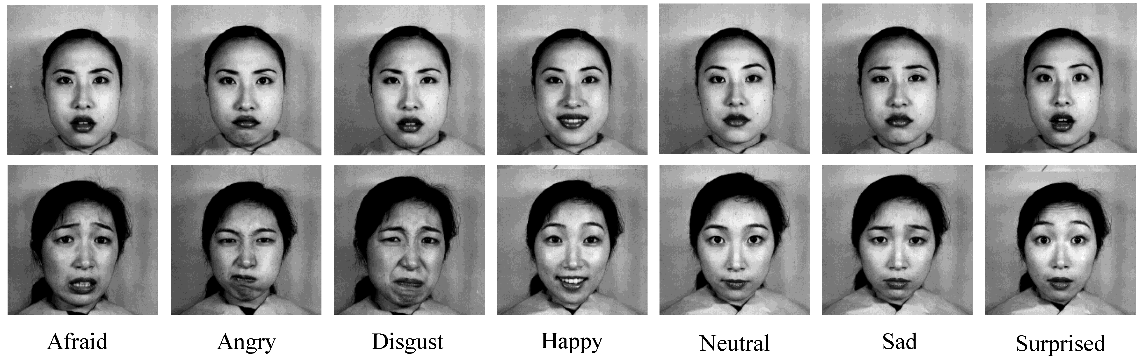
There are few datasets available for the emotion recognition problem; among those, Karolinska Directed Emotional Faces (KDEF) [75] and Japanese Female Facial Expression (JAFFE) [76] datasets are well-known and considered in this study. Images of the datasets are categorized into seven different emotion classes: Afraid (AF), Angry (AN), Disgusted (DI), Sad (SA), Happy (HA), Surprised (SU), and Neutral (NE). The brief description and selection motivation of the datasets are given below.
The KDEF [75] dataset (also refer as KDEF for simplicity, henceforth) was developed by Karolinska Institute, Department of Clinical Neuroscience, Section of Psychology, Stockholm, Sweden. The dataset images were collected in a lab environment, so the emotion of the participants was artificially created. Specifically, the purpose of the dataset was to use for perception memory emotion attention, and backward masking experiment. Although the primary goal of the material was not emotion classification, it is popular for such a task because medical and psychological issues sometimes related to emotion. The dataset contains 4900 images of 70 individuals, each expressing seven emotional states. Photos of an individual were taken from five different angles, which resemble frontal (i.e., strait) view and four different profile views (full left, half left, full right, and half right). In the angular value variation point of view, images are from −90° (full left) to +90° (full right). In a full left or full right profile view, one side of the face with only one eye and ear is visible and makes FER more challenging. Some sample images from the KDEF dataset are shown in Figure 5. FER from the dataset is challenging due to the diversity in images with different profile views along with the frontal view. Profile views mimic the expectation of FER from different angular positions, and therefore, the complete dataset is considered in this study to evaluate the efficiency of the proposed method for such critical cases, which is necessary for industrial applications. Moreover, a few studies are available with the dataset, but they are mostly based on 980 frontal images (e.g., [17,33,60]).
The JAFFE [76] dataset (or JAFFE for simplicity) contains images of the Japanese female models that were taken at the Psychology Department at Kyushu University. The dataset is also collected in a controlled environment for producing facial expressions. Moreover, this dataset contains local facial variation. The JAFFE dataset is comparatively small in size with only 213 frontal images of 10 individuals; some sample images from it are shown in Figure 6. This dataset is chosen to see how a small dataset responds to training the model. Moreover, a large number of studies used the JAFFE dataset to evaluate FER models (e.g., [45,46,51]).
5.2. Experimental Setup
OpenCV [77] is used in this study for cropping the face. The images were resized into 224 × 224, which is the default input size of the pre-trained DCNN models. The parameters of the Adam optimizer are considered as learning rate: 0.0005, beta1: 0.9, and beta2: 0.009. On the other hand, we carefully applied only a small amount of augmentation to the data, and augmentation settings are: Rotation: (−10° to 10°), Scaling factor: ×1.1, Horizontal Flip. Applying such a small transformation to the original image is shown to improve the accuracy.
Experiments conducted separating training and test sets in two different modes: (i) 90% of available images of a benchmark dataset (KDEF or JAFFE) are randomly used as training set, and the rest 10% images are reserved as the test set, and (ii) a 10-Fold Cross-Validation (CV). In a 10-Fold CV, the available images are divided into ten equal (or nearly equal) sets, and the outcome is an average of ten individual runs when each time a particular set was considered as a test set while the remaining nine sets are used for the training purpose. Since the aim of any recognition system is to get a proper response to unseen data, test set accuracy is considered as the performance measure. We trained the model in python with Keras [78] and Tensorflow backend. The experiments were conducted on a PC with a CPU of 3.5 GHz, RAM of 16 GB in the Windows environment.
5.3. Experimental Results and Analysis
This section investigates the efficiency of the proposed model on the benchmark datasets. Since CNN is the building block of the proposed model, at first, a set of comprehensive experiments is conducted with standard CNN to identify the baseline performance. Then, the effects of different fine-tuning modes are investigated with VGG-16. Finally, the performance of the proposed model is tested with different pre-trained DCNN models.
Table 1 presents the test set accuracies for standard CNN with two layers with 3 × 3 size kernel and 2 × 2 MaxPooling for various input sizes from 360 × 360 to 48 × 48 on both KDEF and JAFFE datasets. The size of the test was randomly selected 10% of the available data. The presented results for a particular setting are the best test set accuracies for a total of 50 iterations. It is observed from the table that a larger input image size tends to give better accuracy up to a maximum for both the datasets. As an example, the achieved accuracy on KDEF is 73.87% for an input image size of 360 × 360; whereas, the accuracy is 61.63% for an input size of 48 × 48 for the same dataset. A bigger image has more information, and a system should do well in classifying larger images. However, the best-achieved accuracy did not achieve at the biggest input size (i.e., 360 × 360). Rather, the best accuracies were achieved for both datasets for image size 128 × 128. The reason is that the model is suitable to fit such input size image data, and a larger input size requires more data as well as a larger model to get better performance. The motivation behind the proposed approach is to use the deeper CNN models with TL on a pre-trained model, which minimizes over fittings when trained with a small dataset.
As fine-tuning and its mode are important in the proposed TL-based system, experiments were conducted with different fine-tuning modes for better understanding. Table 2 presents the test set (for randomly selected 10% of the data) accuracies of the proposed model with VGG-16 for the different fine-tuning modes on KDEF and JAFFE datasets. Total training iteration was 50 in any fine-tuning mode; in the case of the entire model, dense layers are trained for 10 iterations first, and the rest 40 iterations are distributed for the addition of Conv blocks of the pre-trained base. For a better understanding of the effectiveness of the proposed TL-based approach, results are also presented for training the whole model from scratch (i.e., with randomly initialized) for 50 iterations. From the table, it is observed that fine-tuning of dense layers and VGG-16 Block 5 is much better than fine-tuning dense layers only, which indicates the fine-tuning of the last block (here Block 5) of the pre-trained model is essential. Again, full VGG-16 Base consideration (i.e., entire model) in fine-tuning is better than considering Block 5 only. The best-achieved accuracies for KDEF and JAFFE datasets are 93.47% and 100%, respectively. On the other hand, training the whole model from scratch shows very low accuracies with respect to TL-based fine-tuning mode, and the achieved test set accuracies are 23.35% and 37.82% for KDEF and JAFFE datasets, respectively. Results presented in the table clearly revealed the proficiency of the proposed TL approach as well as the effectiveness of fine-tuning a portion from the pre-trained DCNN model.
To identify the best suited model, the proposed approach is investigated for eight different pre-trained DCNN models: VGG-16, VGG-19-BN, ResNet-18, ResNet-34, ResNet-50, ResNet-152, Inception-v3 and DenseNet-161. The number with the model’s name represents the depth of that model; therefore, the selected models are diverse with varying depth sizes. The experiments conducted for both randomly selected 10% data as a test (i.e., 90% as the training set) and 10-Fold CV; and test set accuracies with 50 iterations in fine-tuning are presented in Table 3. For the JAFFE dataset, 100% accuracy is achieved by all the models on the selected 10% test data case and the accuracy varied from 97.62% to 99.52% for the 10-Fold CV case. On the other hand, for the KDEF dataset, accuracy varied from 93.47% to 98.78% on 10% of selected test data and 93.02% to 96.51% for the 10-Fold CV case. The size of the KDEF dataset is much larger than JAFFE as well as contains profile view images; therefore, slightly lower accuracy than JAFFE is logical.
It is remarkable from Table 3 that a relatively deeper model performed better. For example, ResNet-152 is always better than its less deep model ResNet-18; the models achieved test set accuracies on KDEF for 10-Fold CV case 96.18% and 93.98%, respectively. Among the considered pre-trained DCNN models, DenseNet-161 is the deepest model and outperformed other models for both datasets. In 10 runs for 10-Fold CV, the model misclassified only six samples among selected 490 test samples (and shown an accuracy of (490 − 6)/490 = 98.78%) for KDEF and it misclassified only one sample case on JAFFE. Table 4 shows the emotion category-wise classification on 490 (=7 × 70) test images of the KDEF dataset by DenseNet-161. Three images in afraid are misclassified as surprised; two images in surprised are misclassified as afraid, and one image in sad is misclassified as disgusted.
Table 5 shows the images which are misclassified by DenseNet-161 and analyzed for better realization of proficiency of the proposed approach. All six misclassified images from KDEF are profile views, and three (sl. 2, 3, and 4) of them are full right views, which complicated the recognition. For the first and the second images from KDEF, the original expression is afraid but predicted as surprised. In both images, the mouth is well extended and open, just like a surprised face. In addition, the widened eye is a feature of surprise. It is difficult even for humans to identify expressions of afraid from facial images. Alternatively, the misclassification of the third image as disgust is logical as it is a profile view (i.e., only one side on the face is visible), so the expression appears to be disgust. The eyes in this image look shrunken, which is similar to disgust. Though the mouth is too exaggerated to be classed as sad, the expression is almost indistinguishable by an algorithm as well as by humans. The remaining three KDEF images share similar cases of misclassification. Finally, the only misclassified image from JAFEE is also difficult to recognize as afraid, while the open mouth looks like surprised.
5.4. Results Comparison with Existing Methods
This section compares the performance of the proposed FER method with the prominent existing methods on emotion recognition using the KDEF and JAFFE datasets. Along with test set recognition accuracy, training and test data separation and distinguished properties of the individual methods are also presented in Table 6 for better understanding. Both classical methods and deep learning-based methods are included in the analysis. Most of the existing methods use the JAFFE dataset; the dataset is relatively small in size with only 213 samples, and eventually, few methods considered 210 samples. On the other hand, KDEF dataset is relatively large, with 4900 images containing both frontal and profile views. Only a few recent studies used this dataset, but they selected only 980 frontal images [17,34,35], or a smaller number of images [52] rather than the complete dataset. It is noteworthy that images with only frontal views are easy to classify than images with both frontal and profile views. Different strategies for separating training and test samples were used in existing studies as listed up in the table. Moreover, each individual method’s significance with technique (used in feature selection and classification) presented in the comparison table is helpful to understand the proficiency of the techniques.
The proposed method with DenseNet-161 is considered for performance comparison in Table 6 as it showed the best accuracy (in Table 3) among the considered eight DCNN models. It is observed from Table 6 that the proposed method outperformed any conventional feature-based method for both KDEF and JAFFE datasets. For JAFFE, among the feature-based methods, the pioneering work incorporating face recognition [48] is still shown to have achieved the best recognition accuracy; the achieved recognition accuracy is 98.98% for equal training and test set division. In the 10-Fold CV case, the method with feature representation using DWT with 2D-LDA and classification using SVM [49] shows the best accuracy of 95.70%. On the other hand, the proposed method achieved an accuracy of 99.52% in 10-Fold CV on JAFFE, which is much better than any other feature-based method; moreover, the accuracy is 100% on randomly selected 10% test samples. In regard of KDEF dataset, the proposed method achieved an accuracy of 98.78% (on randomly selected 10% test samples) considering all 4900 samples and outperformed the existing methods. Notably, accuracy on 10% test samples is 82.40% by [17] considering only selected 980 frontal images, and the efficiency is inferior to the proposed method.
Since the proposed FER is based on the DCNN model through TL, its performance comparison with other deep learning methods, especially CNN-based methods, is more appropriate. The work with SCAE plus CNN [36] shows an accuracy of 92.52% on the KDEF dataset while considering frontal images only. The hybrid CNN and RNN method [56] shows an accuracy of 94.91% on the JAFFE dataset. On the other hand, an accuracy of 98.63% is shown by the method with facial image enhancement using contrast limited adaptive histogram equalization (CLAHE) algorithm, feature extraction using DWT, and then classification using CNN [24]. According to the achieved performance, the proposed method outperformed any other deep learning-based method and revealed the effectiveness of the proposed TL-based approach for FER.
6. Discussion
Emotion recognition from facial images in an uncontrolled environment (e.g., public places), where it is not always possible to acquire frontal view images, is becoming important nowadays for a secure and safe life, smart living, and a smart society. Towards this goal, a robust FER is essential, where emotion recognition from diverse facial views, especially views from various angles, is possible. Profile views from various angles do not show landmark features of the frontal view, and the traditional feature extraction methods are unable to extract facial expression features from the profile views. Therefore, FER from the high-resolution facial image using the DCNN model is considered as the only option to address such a challenging task. The TL-based approach is considered in the proposed FER system: a pre-trained DCNN is made compatible with FER replacing its upper layers with the dense layer(s) to fine-tune the model with facial emotion data. The pipeline training strategy in fine-tuning is the distinguishable feature of the proposed method: the dense layers are tuned first, followed by tuning other DCNN blocks successively.
The proposed method has shown remarkable performance in evaluation on the benchmark datasets with both frontal and profile views. The JAFFE dataset contains frontal views only, and the KDEF dataset contains profile views taken from four different angles along with frontal views. In the full left/right profile view of KDEF, one side of the face with only one eye and ear is visible; thus, the recognition task becomes complex. We felt that the experiments on the two diverse datasets are adequate for proficiency justification, and the proposed method is expected to perform well on other datasets. However, datasets with low-resolution images or with the highly imbalanced case will need additional preprocessing and appropriate modification in the method, which remains a subject for future study. Furthermore, working with images from the uncontrolled environment or video sequences also remains a future study.
As generalization ability (performance on unseen data) is an essential attribute in the machine learning paradigm, the test set concept (samples that are not used in any training step) is used to validate the proposed model. A fixed number of samples reservation from available data and cross-validation (reserve all the samples in the round) are the two popular ways to maintain the test set. Both the methods were considered in the present study, while it is common to follow anyone. The test set was only used for the final validation purposes of the proposed model. The proposed method has outperformed the existing ones based on the achieved test set accuracies. It is noteworthy that the proposed method misclassified only a few images with confusing views, and the overall recognition accuracy remains remarkably high. Therefore, the method proposed in this paper is promising for a practical scenario where the classification of non-frontal or angularly taken images is prevailing.
The parameters’ value selection is a fundamental task for any machine learning system. In the proposed FER model, only the upper dense layers of the pre-trained deep CNN are replaced by some appropriate layers. The hyperparameters (e.g., the number of dense layers, neurons in each layer, and fine-tuning learning parameters) were chosen based on several trials stressing the pipeline training issue. There is a scope to further optimizing every parameter of a particular DCNN model for each dataset that might enhance the performance of the proposed method.
7. Conclusions
In this study, an efficient DCNN using TL with pipeline tuning strategy has been proposed for emotion recognition from facial images. According to the experimental results, using eight different pre-trained DCNN models on well-known KDEF and JAFFE emotion datasets with different profile views, the proposed method shows very high recognition accuracy. In the present study, experiments conducted with general settings regardless of the pre-trained DCNN model for simplicity and a few confusing facial images, mostly profile views, are misclassified. Further fine-tuning hyperparameters of individual pre-trained models and extending special attention to profile views might enhance the classification accuracy. The current research, especially the performance with profile views, will be compatible with broader real-life industry applications, such as monitoring patients in the hospital or surveillance security. Moreover, the idea of facial emotion recognition may be extended to emotion recognition from speech or body movements to cover emerging industrial applications.
Author Contributions
Conceptualization, M.A.H.A., N.S. and T.S.; methodology, M.A.H.A. and S.R.; software: S.R.; writing—original draft preparation, M.A.H.A., S.R., and N.S.; writing—review and editing, M.A.H.A., N.S. and M.A.S.K. All authors have read and agreed to the published version of the manuscript.
Funding
The APC was funded by Tetsuya Shimamura.
Conflicts of Interest
The authors declare no conflict of interest.
References
- Ekman, P. Cross-Cultural Studies of Facial Expression. Darwin and Facial Expression; Malor Books: Los Altos, CA, USA, 2006; pp. 169–220. [Google Scholar]
- Ekman, P.; Friesen, W.V. Constants across cultures in the face and emotion. J. Pers. Soc. Psychol. 1971, 17, 124–129. [Google Scholar] [CrossRef] [Green Version]
- Avila, A.R.; Akhtar, Z.; Santos, J.F.; O’Shaughnessy, D.; Falk, T.H. Feature Pooling of Modulation Spectrum Features for Improved Speech Emotion Recognition in the Wild. IEEE Trans. Affect. Comput. 2021, 12, 177–188. [Google Scholar] [CrossRef]
- Fridlund, A.J. Human facial expression: An evolutionary view. Nature 1995, 373, 569. [Google Scholar]
- Soleymani, M.; Pantic, M.; Pun, T. Multimodal Emotion Recognition in Response to Videos. IEEE Trans. Affect. Comput. 2012, 3, 211–223. [Google Scholar] [CrossRef] [Green Version]
- Noroozi, F.; Marjanovic, M.; Njegus, A.; Escalera, S.; Anbarjafari, G. Audio-Visual Emotion Recognition in Video Clips. IEEE Trans. Affect. Comput. 2019, 10, 60–75. [Google Scholar] [CrossRef]
- Ekman, P.; Friesen, W.V. Measuring facial movement. Environ. Psychol. Nonverbal Behav. 1976, 1, 56–75. [Google Scholar] [CrossRef]
- Ekman, P. Universal Facial Expressions of Emotion. Calif. Ment. Health 1970, 8, 151–158. [Google Scholar]
- Suchitra, P.S.; Tripathi, S. Real-time emotion recognition from facial images using Raspberry Pi II. In Proceedings of the 2016 3rd International Conference on Signal Processing and Integrated Networks (SPIN), Noida, India, 11–12 February 2016; pp. 666–670. [Google Scholar] [CrossRef]
- Yaddaden, Y.; Bouzouane, A.; Adda, M.; Bouchard, B. A new approach of facial expression recognition for ambient assisted living. In Proceedings of the 9th ACM International Conference on PErvasive Technologies Related to Assistive Environments —PETRA, Corfu Island, Greece, 29 June–1 July 2016; Volume 16, pp. 1–8. [Google Scholar] [CrossRef]
- Fernández-Caballero, A.; Martínez-Rodrigo, A.; Pastor, J.M.; Castillo, J.C.; Lozano-Monasor, E.; López, M.T.; Zangróniz, R.; Latorre, J.M.; Fernández-Sotos, A. Smart environment architecture for emotion detection and regulation. J. Biomed. Inf. 2016, 64, 55–73. [Google Scholar] [CrossRef]
- Wingate, M. Prevalence of Autism Spectrum Disorder among children aged 8 years-autism and developmental disabilities monitoring network, 11 sites, United States, 2010. MMWR Surveill. Summ. 2014, 63, 1–21. [Google Scholar]
- Thonse, U.; Behere, R.V.; Praharaj, S.K.; Sharma, P.S.V.N. Facial emotion recognition, socio-occupational functioning and expressed emotions in schizophrenia versus bipolar disorder. Psychiatry Res. 2018, 264, 354–360. [Google Scholar] [CrossRef]
- Pantic, M.; Valstar, M.; Rademaker, R.; Maat, L. Web-Based Database for Facial Expression Analysis. In Proceedings of the 2005 IEEE International Conference on Multimedia and Expo, Amsterdam, The Netherlands, 6 July 2005; pp. 317–321. [Google Scholar] [CrossRef] [Green Version]
- Gross, R.; Matthews, I.; Cohn, J.; Kanade, T.; Baker, S. Multi-PIE. Image Vis. Comput. 2010, 28, 807–813. [Google Scholar] [CrossRef]
- O’Toole, A.J.; Harms, J.; Snow, S.L.; Hurst, D.R.; Pappas, M.R.; Ayyad, J.H.; Abdi, H. A video database of moving faces and people. IEEE Trans. Pattern Anal. Mach. Intell. 2005, 27, 812–816. [Google Scholar] [CrossRef] [PubMed]
- Liew, C.F.; Yairi, T. Facial Expression Recognition and Analysis: A Comparison Study of Feature Descriptors. IPSJ Trans. Comput. Vis. Appl. 2015, 7, 104–120. [Google Scholar] [CrossRef] [Green Version]
- Ko, B.C. A Brief Review of Facial Emotion Recognition Based on Visual Information. Sensors 2018, 18, 401. [Google Scholar] [CrossRef] [PubMed]
- Alom, M.Z.; Taha, T.M.; Yakopcic, C.; Westberg, S.; Sidike, P.; Nasrin, M.S.; Hasan, M.; Van Essen, B.C.; Awwal, A.A.S.; Asari, V.K. A State-of-the-Art Survey on Deep Learning Theory and Architectures. Electronics 2019, 8, 292. [Google Scholar] [CrossRef] [Green Version]
- Sahu, M.; Dash, R. A Survey on Deep Learning: Convolution Neural Network (CNN). In Smart Innovation, Systems and Technologies; Springer: Singapore, 2021; Volume 153, pp. 317–325. [Google Scholar]
- Mollahosseini, A.; Chan, D.; Mahoor, M.H. Going deeper in facial expression recognition using deep neural networks. In Proceedings of the 2016 IEEE Winter Conference on Applications of Computer Vision (WACV), Lake Placid, NY, USA, 7–10 March 2016; pp. 1–10. [Google Scholar] [CrossRef] [Green Version]
- Zhao, X.; Shi, X.; Zhang, S. Facial Expression Recognition via Deep Learning. IETE Tech. Rev. 2015, 32, 347–355. [Google Scholar] [CrossRef]
- Li, J.; Huang, S.; Zhang, X.; Fu, X.; Chang, C.-C.; Tang, Z.; Luo, Z. Facial Expression Recognition by Transfer Learning for Small Datasets. In Advances in Intelligent Systems and Computing; Springer: Berlin/Heidelberg, Germany, 2020; Volume 895, pp. 756–770. [Google Scholar]
- Bendjillali, R.I.; Beladgham, M.; Merit, K.; Taleb-Ahmed, A. Improved Facial Expression Recognition Based on DWT Feature for Deep CNN. Electronics 2019, 8, 324. [Google Scholar] [CrossRef] [Green Version]
- Ngoc, Q.T.; Lee, S.; Song, B.C. Facial Landmark-Based Emotion Recognition via Directed Graph Neural Network. Electronics 2020, 9, 764. [Google Scholar] [CrossRef]
- Pranav, E.; Kamal, S.; Chandran, C.S.; Supriya, M. Facial emotion recognition using deep convolutional neural network. In Proceedings of the 2020 6th International Conference on Advanced Computing and Communication Systems (ICACCS), Coimbatore, India, 6–7 March 2020; pp. 317–320. [Google Scholar] [CrossRef]
- Khan, A.; Sohail, A.; Zahoora, U.; Qureshi, A.S. A survey of the recent architectures of deep convolutional neural networks. Artif. Intell. Rev. 2020, 53, 5455–5516. [Google Scholar] [CrossRef] [Green Version]
- Kolen, J.F.; Kremer, S.C. Gradient Flow in Recurrent Nets: The Difficulty of Learning LongTerm Dependencies. In A Field Guide to Dynamical Recurrent Networks; Wiley-IEEE Press: Hoboken, NJ, USA, 2010; pp. 237–243. [Google Scholar]
- Simonyan, K.; Zisserman, A. Very deep convolutional networks for large-scale image recognition. arXiv 2014, arXiv:1409.1556. [Google Scholar]
- Szegedy, C.; Vanhoucke, V.; Ioffe, S.; Shlens, J.; Wojna, Z. Rethinking the inception architecture for computer vision. In Proceedings of the 2016 IEEE Conference on Computer Vision and Pattern Recognition (CVPR), Las Vegas, NV, USA, 27–30 June 2016; pp. 2818–2826. [Google Scholar] [CrossRef] [Green Version]
- Szegedy, C.; Liu, W.; Jia, Y.; Sermanet, P.; Reed, S.; Anguelov, D.; Erhan, D.; Vanhoucke, V.; Rabinovich, A. Going deeper with convolutions. In Proceedings of the 2015 IEEE Conference on Computer Vision and Pattern Recognition (CVPR), Boston, MA, USA, 7–12 June 2015; pp. 1–9. [Google Scholar] [CrossRef] [Green Version]
- Chollet, F. Xception: Deep learning with depthwise separable convolutions. In Proceedings of the 2017 IEEE Conference on Computer Vision and Pattern Recognition (CVPR), Honolulu, HI, USA, 21–26 July 2017; pp. 1800–1807. [Google Scholar] [CrossRef] [Green Version]
- He, K.; Zhang, X.; Ren, S.; Sun, J. Deep Residual Learning for Image Recognition. In Proceedings of the 2016 IEEE Conference on Computer Vision and Pattern Recognition (CVPR), Las Vegas, NV, USA, 27–30 June 2016; pp. 770–778. [Google Scholar] [CrossRef] [Green Version]
- Huang, G.; Liu, Z.; van der Maaten, L.; Weinberger, K.Q. Densely Connected Convolutional Networks. In Proceedings of the 2017 IEEE Conference on Computer Vision and Pattern Recognition (CVPR), Honolulu, HI, USA, 21–26 July 2017; pp. 2261–2269. [Google Scholar] [CrossRef] [Green Version]
- Alshamsi, H.; Kepuska, V.; Meng, H. Real time automated facial expression recognition app development on smart phones. In Proceedings of the 2017 8th IEEE Annual Information Technology, Electronics and Mobile Communication Conference (IEMCON), Vancouver, BC, Canada, 3–5 October 2017; pp. 384–392. [Google Scholar] [CrossRef] [Green Version]
- Alshamsi, H.; Kepuska, V.; Meng, H. Stacked deep convolutional auto-encoders for emotion recognition from facial expressions. Proc. Int. Jt. Conf. Neural Netw. 2017, 2017, 1586–1593. [Google Scholar] [CrossRef]
- Oquab, M.; Bottou, L.; Laptev, I.; Sivic, J. Learning and transferring mid-level image representations using convolutional neural networks. In Proceedings of the 2014 IEEE Conference on Computer Vision and Pattern Recognition, Columbus, OH, USA, 24–27 June 2014; pp. 1717–1724. [Google Scholar] [CrossRef] [Green Version]
- Yosinski, J.; Clune, J.; Bengio, Y.; Lipson, H. How transferable are features in deep neural networks? In Advances in Neural Information Processing Systems 27; Ghahramani, Z., Welling, M., Cortes, C., Lawrence, N.D., Weinberger, K.Q., Eds.; Curran Associates, Inc.: Red Hook, NY, USA, 2014; pp. 3320–3328. [Google Scholar]
- Torrey, L.; Shavlik, J. Transfer Learning. In Machine Learning Applications and Trends; IGI Global: Hershey, PA, USA, 2010; pp. 242–264. [Google Scholar]
- Rawat, W.; Wang, Z. Deep Convolutional Neural Networks for Image Classification: A Comprehensive Review. Neural Comput. 2017, 29, 2352–2449. [Google Scholar] [CrossRef]
- Huang, Y.; Chen, F.; Lv, S.; Wang, X. Facial Expression Recognition: A Survey. Symmetry 2019, 11, 1189. [Google Scholar] [CrossRef] [Green Version]
- Li, S.; Deng, W. Deep Facial Expression Recognition: A Survey. IEEE Trans. Affect. Comput. 2020. [Google Scholar] [CrossRef] [Green Version]
- Xiao, X.Q.; Wei, J. Application of wavelet energy feature in facial expression recognition. In Proceedings of the 2007 International Workshop on Anti-Counterfeiting, Security and Identification (ASID), Xiamen, China, 16–18 April 2007; pp. 169–174. [Google Scholar] [CrossRef]
- Zhao, L.; Zhuang, G.; Xu, X. Facial expression recognition based on PCA and NMF. In Proceedings of the 2008 7th World Congress on Intelligent Control and Automation, Chongqing, China, 25–27 June 2008; pp. 6826–6829. [Google Scholar] [CrossRef]
- Feng, X.; Pietikainen, M.; Hadid, A. Facial expression recognition based on local binary patterns. Pattern Recognit. Image Anal. 2007, 17, 592–598. [Google Scholar] [CrossRef]
- Zhi, R.; Ruan, Q. Facial expression recognition based on two-dimensional discriminant locality preserving projections. Neurocomputing 2008, 71, 1730–1734. [Google Scholar] [CrossRef]
- Lee, C.-C.; Shih, C.-Y.; Lai, W.-P.; Lin, P.-C. An improved boosting algorithm and its application to facial emotion recognition. J. Ambient. Intell. Humaniz. Comput. 2012, 3, 11–17. [Google Scholar] [CrossRef]
- Chang, C.-Y.; Huang, Y.-C. Personalized facial expression recognition in indoor environments. In Proceedings of the 2010 International Joint Conference on Neural Networks (IJCNN), Barcelona, Spain, 18–23 July 2010; pp. 1–8. [Google Scholar] [CrossRef]
- Shih, F.Y.; Chuang, C.-F.; Wang, P.S.P. Performance comparisons of facial expression recognition in JAFFE database. Int. J. Pattern Recognit. Artif. Intell. 2008, 22, 445–459. [Google Scholar] [CrossRef]
- Shan, C.; Gong, S.; McOwan, P.W. Facial expression recognition based on Local Binary Patterns: A comprehensive study. Image Vis. Comput. 2009, 27, 803–816. [Google Scholar] [CrossRef] [Green Version]
- Jabid, T.; Kabir, H.; Chae, O. Robust Facial Expression Recognition Based on Local Directional Pattern. ETRI J. 2010, 32, 784–794. [Google Scholar] [CrossRef]
- Joseph, A.; Geetha, P. Facial emotion detection using modified eyemap–mouthmap algorithm on an enhanced image and classification with tensorflow. Vis. Comput. 2020, 36, 529–539. [Google Scholar] [CrossRef]
- Pons, G.; Masip, D. Supervised Committee of Convolutional Neural Networks in Automated Facial Expression Analysis. IEEE Trans. Affect. Comput. 2018, 9, 343–350. [Google Scholar] [CrossRef]
- Wen, G.; Hou, Z.; Li, H.; Li, D.; Jiang, L.; Xun, E. Ensemble of Deep Neural Networks with Probability-Based Fusion for Facial Expression Recognition. Cogn. Comput. 2017, 9, 597–610. [Google Scholar] [CrossRef]
- Ding, H.; Zhou, S.K.; Chellappa, R. FaceNet2ExpNet: Regularizing a deep face recognition net for expression recognition. In Proceedings of the 2017 12th IEEE International Conference on Automatic Face & Gesture Recognition (FG 2017), Washington, DC, USA, 30 May–3 June 2017; pp. 118–126. [Google Scholar] [CrossRef] [Green Version]
- Jain, N.; Kumar, S.; Kumar, A.; Shamsolmoali, P.; Zareapoor, M. Hybrid deep neural networks for face emotion recognition. Pattern Recognit. Lett. 2018, 115, 101–106. [Google Scholar] [CrossRef]
- Shaees, S.; Naeem, H.; Arslan, M.; Naeem, M.R.; Ali, S.H.; Aldabbas, H. Facial Emotion Recognition Using Transfer Learning. In Proceedings of the 2020 International Conference on Computing and Information Technology (ICCIT-1441), Tabuk, Saudi Arabia, 9–10 September 2020; pp. 1–5. [Google Scholar] [CrossRef]
- Liliana, D.Y. Emotion recognition from facial expression using deep convolutional neural network. J. Phys. Conf. Ser. 2019, 1193, 012004. [Google Scholar] [CrossRef] [Green Version]
- Shi, M.; Xu, L.; Chen, X. A Novel Facial Expression Intelligent Recognition Method Using Improved Convolutional Neural Network. IEEE Access 2020, 8, 57606–57614. [Google Scholar] [CrossRef]
- Jin, X.; Sun, W.; Jin, Z. A discriminative deep association learning for facial expression recognition. Int. J. Mach. Learn. Cybern. 2019, 11, 779–793. [Google Scholar] [CrossRef]
- Porcu, S.; Floris, A.; Atzori, L. Evaluation of Data Augmentation Techniques for Facial Expression Recognition Systems. Electronics 2020, 9, 1892. [Google Scholar] [CrossRef]
- Akhand, M.A.H.; Ahmed, M.; Rahman, M.M.H.; Islam, M. Convolutional Neural Network Training incorporating Rotation-Based Generated Patterns and Handwritten Numeral Recognition of Major Indian Scripts. IETE J. Res. 2018, 64, 176–194. [Google Scholar] [CrossRef] [Green Version]
- Antonellis, G.; Gavras, A.G.; Panagiotou, M.; Kutter, B.L.; Guerrini, G.; Sander, A.C.; Fox, P.J. Shake Table Test of Large-Scale Bridge Columns Supported on Rocking Shallow Foundations. J. Geotech. Geoenviron. Eng. 2015, 141, 04015009. [Google Scholar] [CrossRef]
- Zeiler, M.D.; Fergus, R. Visualizing and Understanding Convolutional Networks. In Proceedings of the European Conference on Computer Vision (ECCV 2014), Zurich, Switzerland, 6–12 September 2014; pp. 818–833. [Google Scholar] [CrossRef] [Green Version]
- Nair, V.; Hinton, G.E. Rectified linear units improve restricted boltzmann machines. In Proceedings of the 27th International Conference on Machine Learning, Haifa, Israel, 21–24 June 2010; pp. 807–814. [Google Scholar]
- Roos, P.C.; Schuttelaars, H.M. Resonance properties of tidal channels with multiple retention basins: Role of adjacent sea. Ocean. Dyn. 2015, 65, 311–324. [Google Scholar] [CrossRef] [Green Version]
- Razavian, A.S.; Azizpour, H.; Sullivan, J.; Carlsson, S. CNN Features Off-the-Shelf: An Astounding Baseline for Recognition. In Proceedings of the 2014 IEEE Conference on Computer Vision and Pattern Recognition Workshops, Columbus, OH, USA, 23–28 June 2014; pp. 512–519. [Google Scholar] [CrossRef] [Green Version]
- Bukar, A.M.; Ugail, H. Automatic age estimation from facial profile view. IET Comput. Vis. 2017, 11, 650–655. [Google Scholar] [CrossRef] [Green Version]
- Mahendran, A.; Vedaldi, A. Visualizing Deep Convolutional Neural Networks Using Natural Pre-images. Int. J. Comput. Vis. 2016, 120, 233–255. [Google Scholar] [CrossRef] [Green Version]
- Bengio, Y. Earning Deep Architectures for AI. Found. Trends Mach. Learn. 2009, 2, 1–127. [Google Scholar] [CrossRef]
- Marcelino, P. Solve any Image Classification Problem Quickly and Easily. 2018. Available online: https://www.kdnuggets.com/2018/12/solve-image-classification-problem-quickly-easily.html (accessed on 1 April 2021).
- Kingma, D.P.; Ba, J. Adam: A Method for Stochastic Optimization. arXiv 2014, arXiv:1412.6980. [Google Scholar]
- Bartlett, P.L.; Hazan, E.; Rakhlin, A. Adaptive Online Gradient Descent. Adv. Neural Inf. Process. Syst. 2007, 20, 1–8. [Google Scholar]
- Tieleman, T.; Hinton, G.E.; Srivastava, N.; Swersky, K. RMSProp: Divide the gradient by a running average of its recent magnitude. COURSERA Neural Netw. Mach. Learn. 2012, 4, 26–31. [Google Scholar]
- Calvo, M.G.; Lundqvist, D. Facial expressions of emotion (KDEF): Identification under different display-duration conditions. Behav. Res. Methods 2008, 40, 109–115. [Google Scholar] [CrossRef] [PubMed] [Green Version]
- Lyons, M.J.; Akamatsu, S.; Kamachi, M.; Gyoba, J.; Budynek, J. The Japanese Female Facial Expression (JAFFE) Database. Available online: http://www.kasrl.org/jaffe_download.html (accessed on 1 February 2021).
- Bradski, G. The OpenCV Library. Dr. Dobb’s J. Softw. Tools 2000, 120, 122–125. [Google Scholar] [CrossRef]
- François, C. Keras: The Python Deep Learning Library. Available online: https://keras.io (accessed on 15 November 2020).
Figure 1.
The generic architecture of a convolutional neural network with two convolutional-pooling layers.
Figure 1.
The generic architecture of a convolutional neural network with two convolutional-pooling layers.

Figure 2.
General architecture of transfer learning-based deep CNN model for emotion recognition.

Figure 3.
Illustration of the proposed FER system based on transfer learning in deep CNN.

Figure 4.
Illustration of the proposed Emotion Recognition model with VGG-16 model plus dense (i.e., fully connected) layers. VGG-16 model is pre-trained on ImageNet dataset. A block with ‘Fine-tune’ mark is essential to fine-tune and a block with ‘Frozen/Fine-tune’ mark is optional to fine-tune.
Figure 4.
Illustration of the proposed Emotion Recognition model with VGG-16 model plus dense (i.e., fully connected) layers. VGG-16 model is pre-trained on ImageNet dataset. A block with ‘Fine-tune’ mark is essential to fine-tune and a block with ‘Frozen/Fine-tune’ mark is optional to fine-tune.

Figure 5.
Sample images from KDEF dataset.

Figure 6.
Sample images from JAFFE dataset.


Table 1.
Test set accuracies of standard CNN with two layers on KDEF and JAFFE datasets for different input size images.
Table 1.
Test set accuracies of standard CNN with two layers on KDEF and JAFFE datasets for different input size images.
| Input Image Size | KDEF | JAFFE |
|---|---|---|
| 360 × 360 | 73.87% | 91.67% |
| 224 × 224 | 73.46% | 87.50% |
| 128 × 128 | 80.81% | 91.67% |
| 64 × 64 | 69.39% | 83.33% |
| 48 × 48 | 61.63% | 79.17% |
Table 2.
Comparison of test set accuracies with VGG-16 for different training modes in fine-tuning.
| Training Mode | KDEF | JAFFE |
|---|---|---|
| Dense Layers only | 77.55% | 91.67% |
| Dense Layers + VGG-16 Block 5 | 91.83% | 95.83% |
| Entire Model (Dense Layers + Full VGG-16 Base) | 93.47% | 100.0% |
| Whole Model from Scratch | 23.35% | 37.82% |
Table 3.
Comparison of the test set accuracies with different pre-trained deep CNN models on KDEF and JAFFE datasets.
Table 3.
Comparison of the test set accuracies with different pre-trained deep CNN models on KDEF and JAFFE datasets.
| Pre-Trained Deep CNN Model | KDEF in Selected 10% Test Samples | KDEF in 10-Fold CV | JAFFE in Selected 10% Test Samples | JAFFE in 10-Fold CV |
|---|---|---|---|---|
| VGG-16 | 93.47% | 93.02 ± 1.48% | 100.0% | 97.62 ± 4.05% |
| VGG-19 | 96.73% | 95.29 ± 1.12% | 100.0% | 98.41 ± 3.37% |
| ResNet-18 | 94.29% | 93.98 ± 0.84% | 100.0% | 98.09 ± 3.33% |
| ResNet-34 | 96.33% | 94.83 ± 0.88% | 100.0% | 98.57 ± 3.22% |
| ResNet-50 | 97.55% | 95.20 ± 0.89% | 100.0% | 99.05 ± 3.01% |
| ResNet-152 | 96.73% | 96.18 ± 1.28% | 100.0% | 99.52 ± 1.51% |
| Inception-v3 | 97.55% | 95.10 ± 0.91% | 100.0% | 99.05 ± 2.01% |
| DenseNet-161 | 98.78% | 96.51 ± 1.08% | 100.0% | 99.52 ± 1.51% |
Table 4.
Classification of each emotion class of KDEF dataset.
| AF | AN | DI | HA | NE | SA | SU | |
|---|---|---|---|---|---|---|---|
| Afraid (AF) | 67 | 0 | 0 | 0 | 0 | 0 | 3 |
| Angry (AN) | 0 | 70 | 0 | 0 | 0 | 0 | 0 |
| Disgusted (DI) | 0 | 0 | 70 | 0 | 0 | 0 | 0 |
| Happy (HA) | 0 | 0 | 0 | 70 | 0 | 0 | 0 |
| Neutral (NE) | 0 | 0 | 0 | 0 | 70 | 0 | 0 |
| Sad (SA) | 0 | 0 | 1 | 0 | 0 | 69 | 0 |
| Surprised (SU) | 2 | 0 | 0 | 0 | 0 | 0 | 68 |
Table 5.
Misclassified images from KDEF and JFEE datasets with their original and predicted class labels.
Table 5.
Misclassified images from KDEF and JFEE datasets with their original and predicted class labels.
| Misclassified Image: True Class → Predicted Class | ||||||
|---|---|---|---|---|---|---|
| Samples from KDEF |  |  |  |  |  |  |
| 1. Afraid → Surprised | 2. Afraid → Surprised | 3. Sad → Disgust | 4. Afraid → Surprised | 5. Surprised → Afraid | 6. Surprised → Afraid | |
| Sample from JAFFE |  | |||||
| 7. Afraid → Surprised | ||||||
Table 6.
Comparison of the accuracy of proposed method with existing works on KDEF and JAFFE datasets.
Table 6.
Comparison of the accuracy of proposed method with existing works on KDEF and JAFFE datasets.
| Work [Ref.], Year | Total Samples: Training and Test Division | Test Set Accuracy (%) | Method’s Significance in Feature Selection and Classification | |
|---|---|---|---|---|
| KDEF | JAFFE | |||
| Zhi and Ruan [46], 2008 | 213: 30-Fold CV | 95.91 | Derived feature vector from 2D discriminant locality preserving projections | |
| Shih el al. [49], 2008 | 213: 10-Fold CV | 95.70 | Feature representation using DWT with 2D-LDA and classification using SVM | |
| Shan et al. [50], 2009 | 213: 10-Fold CV | 81.00 | Feature extraction using statistical local features and LBPs; classification with different variants of SVM | |
| Jabid et al. [51], 2010 | 213: 7-Fold CV | 82.60 | Feature extraction using appearance-based technique and classification with different variants of SVM | |
| Chang and Huang [48], 2010 | 210: 105 + 105 | 98.98 | Incorporated face recognition and used RBF for classification | |
| Lee et al. [47], 2011 | 210: 30-Fold CV | 96.43 | Contourlet Transform for feature extraction and Boosting algorithm for classification | |
| Liew and Yairi, [17], 2015 | KDEF# 980 frontal images: 90% + 10% JAFFE# 213:90% + 10% | 82.40 | 89.50 | feature extracted employing Gabor, Haar, LBP etc. and classify using SVM, KNN, LDA, etc. |
| Alshami el al. [35], 2017 | KDEF# 980 frontal images: 70% + 30% JAFFE# 213: 70% + 30% | 90.80 | 91.90 | Used Facial Landmarks descriptor and Center of Gravity descriptor with SVM |
| Joseph and Geetha [52], 2019 | Selected 478 images: 10-Fold CV | 31.20 | Facial geometry-based feature extraction with different classification methods including SVM, KNN | |
| Standard CNN (Self Implemented) | KDEF# 4900: 90% + 10% JAFFE# 213: 90% + 10% | 80.81 | 91.67 | Standard CNN with fully connected layer for classification |
| Zhao and Zhang [22], 2015 | 213: 10-Fold CV | 90.95 | DBN is used for unsupervised feature learning and NN is used for classification | |
| Ruiz-Garcia et al. [36], 2017 | 980 frontal images: 70% + 30% | 92.52 | Stacked Convolutional Auto-Encoder (SCAE) is used to initialize weights of CNN. | |
| Jain et al. [56], 2018 | 213: 70% + 30% | 94.91 | Hybrid deep learing architecture with CNN and RNN | |
| Bendjillali et al. [24], 2019 | 213: 70% + 30% | 98.63 | Image enhancement, feature extration and classification using CNN | |
| Proposed Method with DenseNet-161 | KDEF# 4900: 90% + 10% JAFFE# 213: 90% + 10% | 98.78 | 100.00 | Transfer leaning on pre-trained Deep CNN model employing a pipeline strategy in fine-tuning |
| KDEF# 4900: 10-Fold CV JAFFE# 213: 10-Fold CV | 96.51 | 99.52 | ||
Publisher’s Note: MDPI stays neutral with regard to jurisdictional claims in published maps and institutional affiliations. |
© 2021 by the authors. Licensee MDPI, Basel, Switzerland. This article is an open access article distributed under the terms and conditions of the Creative Commons Attribution (CC BY) license (https://creativecommons.org/licenses/by/4.0/).
Share and Cite
MDPI and ACS Style
Akhand, M.A.H.; Roy, S.; Siddique, N.; Kamal, M.A.S.; Shimamura, T. Facial Emotion Recognition Using Transfer Learning in the Deep CNN. Electronics 2021, 10, 1036. https://doi.org/10.3390/electronics10091036
AMA Style
Akhand MAH, Roy S, Siddique N, Kamal MAS, Shimamura T. Facial Emotion Recognition Using Transfer Learning in the Deep CNN. Electronics. 2021; 10(9):1036. https://doi.org/10.3390/electronics10091036
Chicago/Turabian StyleAkhand, M. A. H., Shuvendu Roy, Nazmul Siddique, Md Abdus Samad Kamal, and Tetsuya Shimamura. 2021. "Facial Emotion Recognition Using Transfer Learning in the Deep CNN" Electronics 10, no. 9: 1036. https://doi.org/10.3390/electronics10091036
Note that from the first issue of 2016, this journal uses article numbers instead of page numbers. See further details here.