
Optimization Strategy of Configuration and Scheduling for User-Side Energy Storage
by
 ,
,
Yushan Liu
1 ,
,
Qianqian Liu
1,
Huaimin Guan
2,
Xiao Li
1,*,
Daqiang Bi
3,
Yingjun Guo
4 and
Hexu Sun
4,* 1
School of Automation Science and Electrical Engineering, Beihang University, Beijing 100083, China
2
School of Software, Beihang University, Beijing 100083, China
3
State Key Lab of Power Systems, Department of Electrical Engineering, Tsinghua University, Beijing 100084, China
4
School of Electrical Engineering, Hebei University of Science and Technology, Shijiazhuang 050018, China
*
Authors to whom correspondence should be addressed.
Electronics 2022, 11(1), 120; https://doi.org/10.3390/electronics11010120
Submission received: 3 December 2021
/
Revised: 22 December 2021
/
Accepted: 27 December 2021
/
Published: 30 December 2021
(This article belongs to the Special Issue Feature Papers in Power Electronics)
Abstract
:In order to reduce the impact of load power fluctuations on the power system and ensure the economic benefits of user-side energy storage operation, an optimization strategy of configuration and scheduling based on model predictive control for user-side energy storage is proposed in this study. Firstly, considering the cost and benefits of energy storage comprehensively, an energy storage configuration optimization model with the highest annualized net income as the goal is built to determine the parameters for configuring energy storage. Then, with the goal of maximizing the profit during the scheduling period, pre-month scheduling optimization model, day-ahead scheduling optimization model and intra-day scheduling optimization model are established. The goal of the pre-month scheduling optimization model is to determine the maximum monthly demand; part of the scheduling results in the day-ahead scheduling optimization model directly participate in the intra-day scheduling; the intra-day rolling optimization relies on the advantages of real-time feedback and closed-loop scheduling to smooth out power fluctuations caused by load forecast errors. Finally, the configuration and economic benefit of lithium iron phosphate batteries, lead-carbon batteries and sodium-sulfur batteries are analyzed and compared, and scheduling analysis is performed. The simulation results show that the proposed optimization method can cut peaks and fill valleys, ensure the economic benefits of users, and provide guidance for users to invest in energy storage.
1. Introduction
Energy storage can realize the migration of energy in time, and then can adjust the change of electric load. Therefore, it is widely used in smoothing the load power curve, cutting peaks and filling valleys as well as reducing load peaks [1,2,3,4,5,6]. China has also issued corresponding policies to encourage the development of energy storage on the user side, and pointed out that the peak-to-valley difference in electricity prices is expected to be further widened in the future, and the room for users to benefit from additional energy storage will be further expanded. Therefore, the research on the optimal configuration of user-side energy storage has certain practical significance. At the same time, in order to give full play to the advantages of energy storage, efficient scheduling strategies need to be adopted to ensure optimal operation of energy storage and reduce user electricity costs.
There have been some studies on user-side energy storage configuration, but there are few related papers on demand response. Refs. [7,8,9,10] established a capacity market model considering demand response, but failed to conduct in-depth research on energy storage configuration. Ref. [11] established an energy storage investment model under the full life cycle, but did not consider demand response. Ref. [12] established an energy storage operation model, but only considered the peak-to-valley spread arbitrage in the income. Ref. [13] studied energy storage configuration, but did not consider peak shaving revenue in the revenue. Refs. [14,15] established an energy storage system model with the maximum net present value as the objective function, but did not fully consider the benefits of energy storage. Ref. [16] established an energy storage planning and scheduling model, but did not consider the demand response benefits. Ref. [17] proposed an optimization method for energy storage configuration, but only the two-stage electricity revenue was considered in the objective function. Ref. [18] proposed an energy storage configuration model considering the capacity market, but its research focused on foreign capacity markets, which is quite different from China’s market environment. Refs. [19,20] established an energy storage configuration model considering demand management, Refs. [21,22] established an energy storage configuration model with the goal of maximizing net income, and Ref. [23] established a life cycle energy storage model. But none of its benefits involve demand response. The current energy storage configuration model does not fully consider the relevant technical parameters and performance characteristics of energy storage.
Energy storage is mainly involved in energy scheduling as one of the multiple devices in the integrated energy system. Refs. [24,25] optimized energy dispatch for systems including heat storage devices, combined heat and power (CHP) and wind turbines; Ref. [26] established a day-ahead optimal dispatch model for electric–heat–gas coupled systems; Ref. [27] carried out the optimal dispatching of cold, heat and electricity based on energy hub; Ref. [28] carried out coordinated dispatching of systems, including electric energy storage, thermal energy storage, electric heat pump and CHP equipment. In [29], based on the virtual energy storage system, the optimal dispatching of cold, heat and electricity is carried out. The above-mentioned optimal scheduling is carried out based on accurate load forecasting, but in the actual operation of the system, there is a deviation between the forecasted load and the actual load, which is not conducive to the operation of the system. In order to solve the problem of uncertainty in forecasting load, interval planning [30,31], stochastic planning [32], robust planning [33,34], etc. have been widely used. The above methods make scheduling plans for multiple periods in advance, which cannot meet the requirements of online and real-time optimized operation of the system.
Model predictive control (MPC) designs future scheduling plans based on system predictive data and actual system status, and at the same time continuously updates the actual status of the system over time, and performs rolling forward optimization. Only the plan value of the first time period is executed each time, and the control performance is good. Ref. [35] combined MPC method and demand response mechanism to carry out intra-day rolling optimization dispatch of microgrid; Ref. [36] used the MPC method to optimize the dispatch of the blockchain-based microgrid power market; Ref. [37] used the MPC method to perform multi-time-scale scheduling on a microgrid with multiple buildings, which can reduce system costs and stabilize tie-line power fluctuations; Ref. [38] based on the MPC method and consistency theory, the proposed distributed optimal dispatching can solve the problem of solving microgrid clusters; Ref. [39] used the MPC method to regulate the building microgrid system including virtual energy storage, which was robust in uncertain scenarios such as renewable energy output and load forecasting; Ref. [40] used the MPC method to optimize the energy system of the park. The above-mentioned literature uses the MPC method to enhance the robustness of the system, but the above-mentioned systems are all scheduling plans given when the model has an optimal solution, and no solution is given when the model has no optimal solution.
In summary, fully considering the cost and benefits of energy storage and the impact of the uncertainty of load forecast power on the energy scheduling of user systems with additional energy storage, this paper builds a user-side energy storage configuration optimization model that participates in demand response, and proposes an optimization strategy for user-side energy storage scheduling based on MPC. First, it analyzes the life model, cost model and revenue model of energy storage in detail, and builds an energy storage configuration model to solve the rated capacity and rated power of the additional energy storage. Second, under the two-part electricity price mechanism, based on the pre-month load forecast data, a pre-month optimization model with the maximum monthly income as the goal is built to determine the maximum monthly demand. Third, based on the monthly maximum demand value and day-ahead load forecast data, a day-ahead optimization model with the goal of maximizing daily income is built to obtain the charge and discharge power of the energy storage at each moment in the day before. Fourth, based on the results of the above model and the actual load data, the feedback correction is performed, and the energy storage output is optimized using the MPC-based rolling optimization scheduling strategy. Finally, the effectiveness and rationality of the proposed method are verified through simulation. Through the configuration of energy storage, peak shaving and valley filling are realized, the peak load is reduced, the smooth operation of the power grid is ensured and certain economic benefits are brought to users.
2. Energy Storage Model
2.1. Life Model
The life of energy storage is determined by the number of cycles and the depth of discharge. The equivalent operating life T years of a lithium iron phosphate battery is [18]:
where dod is the depth of charge and discharge of energy storage and cy is the average number of cycles of energy storage per year.
2.2. Cost Model
The cost model of energy storage includes installation costs, operation and maintenance costs, and capacity attenuation costs. At the same time, it also considers a regularized function for smoothing the power fluctuations of the grid connection point.
2.2.1. Annual Installation Costs
The cost of energy storage installation includes the battery body, power conversion device, supporting equipment and engineering expenses. The battery investment is proportional to the rated capacity of energy storage, the investment of power conversion device is proportional to the rated power of energy storage, and the costs of supporting equipment and engineering are proportional to the rated capacity of energy storage [19]. Therefore, the annual installation costs C1 of energy storage can be expressed as:
where Ebat is the rated capacity of energy storage; Pbat is the rated power of energy storage; c11 is the price per unit capacity of energy storage; c12 is the price per unit power of energy storage; and r is the discount rate.
2.2.2. Annual Operation and Maintenance Costs
The annual operation and maintenance costs of energy storage are related to the rated power of energy storage. The annual operation and maintenance costs C2 can be expressed as:
where c2 is the operation and maintenance cost per unit power of energy storage.
2.2.3. Energy Storage Capacity Attenuation Costs
Frequent charging and discharging of energy storage will gradually reduce the energy storage capacity, resulting in a decline in energy storage revenue. The amount of energy storage capacity attenuation is determined by the number of cycles and the depth of discharge, so the average annual loss function of energy storage revenue C3 and the annual capacity attenuation of energy storage Crs can be expressed as [19]:
where Dy is the average annual operating days of energy storage; η is the energy storage charge and discharge efficiency; efg is the peak-to-valley price difference; efp is the peak-to-average price difference; n is the number of cycles per day for energy storage; SOCmax and SOCmin are the upper and lower limits of the state of charge of energy storage; and δ(dod) is the capacity decay rate per cycle of energy storage at the depth of dod discharge.
2.2.4. Regularization Function for Smoothing the Power Fluctuation of the Grid Connection Point
The power curve of the grid-connected point is smoothed by controlling the charge and discharge power of the energy storage, and the power fluctuation of the grid-connected point is included in the costs in the form of a regularization function. The regularization function C4 can be expressed as:
where εZ is the regularization coefficient of smoothing power; M is the number of months per year; D is the number of days per month; and H is the number of hours per day. Plb(i,j,t) is the grid-connected point power at time t on the j-th day of the i-th month after the energy storage is configured.
2.3. Revenue Model
The revenue model of energy storage includes electricity bill revenue, reduced transformer cost due to peak load reduction, recovery value, demand response benefit, reliability benefit from reduced power outages and government subsidy benefit.
2.3.1. Electricity Revenue
The electricity bill paid by large industrial users consists of two parts: the basic electricity bill and the kilowatt hour electricity bill. The basic electricity bill can be calculated according to the capacity of the transformer, or according to the maximum demand. Users whose basic electricity bill is charged according to the maximum demand shall sign a contract with the power grid company, and the basic electricity bill shall be calculated and collected according to the maximum monthly demand value of the contract. The kilowatt hour electricity bill is calculated and collected according to the user’s actual monthly electricity consumption. Based on the two-part electricity price, taking into account the power supply pressure of the power grid, and using the characteristics of energy storage to cut peaks, the monthly basic electricity bill paid by users can be reduced; At the same time, energy storage transfers the load in the time dimension and utilizes the time-of-use electricity price. “Low storage and high discharge” can save electricity costs.
- (1)
- The basic electricity revenue
This paper calculates the basic electricity bill based on the maximum demand, and the user’s monthly demand electricity bill R billing rules:
where cb is the unit price of the maximum demand; PMM is the monthly maximum demand value signed by the contract; and Pact is the actual measured monthly maximum demand value.
The actual measured maximum demand exceeds 105% of the contractual approved value, and the basic electricity fee for the portion exceeding 105% is doubled. Therefore, energy storage can smooth the power curve of the grid connection point and reduce the maximum demand value through “low storage and high discharge”. The annual basic electricity cost I1 saved is:
where EN(i) is the demand electricity bill for the i-th month without energy storage; and EY(i) is the demand electricity bill for the i-th month with energy storage.
- (2)
- The kilowatt hour electricity revenue
The “low storage and high discharge” of energy storage can transfer the power load. According to the time-of-use tariff mechanism, users can generate revenue from peak shaving and valley filling. Therefore, the annual kilowatt hour electricity cost I2 saved is:
where P(i,j,t) is the absorbed power value of energy storage at time t on the j-th day of the i-th month, negative value for discharging and positive value for charging; and e(t) is the time-of-use electricity price at time t.
2.3.2. Reduced Average Annual Transformer Cost
With fixed power factor and load rate, the transformer parameters configured by the user depend on the annual peak load. In the project planning stage, the annual average transformer cost I3 that can be reduced by reducing the annual load peak can be expressed as:
where α is the ratio of transformer installation cost to equipment cost; c3 is the unit price of the transformer; K is the load factor of the transformer; cosφ is the power factor; Ppeak and P′peak are the user’s original annual load peak value and the annual load peak value after the energy storage is configured.
2.3.3. Recovery Value
After the energy storage is scrapped, it can be recycled to obtain benefits. The average annual recovery value I4 of energy storage can be expressed as:
where γ is the recovery factor and C1 is the annual installation cost.
2.3.4. Demand Response Benefit
Demand response means that when the reliability of the power system is threatened, the user reduces the power load for a specified period of time according to the notification of the power supplier to ensure the safe and stable operation of the power grid system. The revenue I5 obtained by the user from the implementation of the demand response contract each year can be expressed as:
where Pr(j) is the benefit after implementing the demand response contract on the j-th day to reduce the corresponding load and Pu(j) is the penalty paid for defaulting on the j-th day without reducing the load.
2.3.5. Reliability Benefit
Users can install energy storage to improve the reliability of power supply, and the number of power outages can be greatly reduced. The annual reliability benefit I6 brought by energy storage can be expressed as:
where is the user’s profit loss per unit capacity for 1 h of power outage and tt is the average annual outage time of the user’s power outage reduced by adding energy storage to the rated power of the energy storage.
2.3.6. Annual Benefit from Government Subsidies
Suzhou implemented an energy storage subsidy policy in 2019, subsidizing users 0.3 yuan per kilowatt-hour of electricity discharged by energy storage. The annual subsidy benefit I7 is:
where P(i,j,t)− is the discharge power value of energy storage at time t on the j-th day of the i-th month, which is a negative value; eb is the subsidized electricity price per kilowatt-hour.
3. Energy Storage Configuration Model
The energy storage configuration model is used to determine the rated power and rated capacity of the energy storage installed by the user.
3.1. Objective Function
The objective function of the energy storage configuration optimization model is that the annualized net income of energy storage is the highest, and the capacity and power of the user’s additional energy storage are optimized. The objective function G can be expressed as:
where I1 is the annual basic electricity cost saved by energy storage; I2 is the annual electricity cost saved by energy storage; I3 is the annual average transformer cost that can be reduced by reducing the annual load peak; I4 is the average annual recovery value of energy storage; I5 is the revenue that users obtain from the implementation of demand response contracts each year; I6 is the annual reliability benefit of energy storage; I7 is the average annual government subsidy revenue; C1 is the annual installation cost of energy storage; C2 is the annual operation and maintenance cost of energy storage; C3 is the average annual revenue loss function caused by the attenuation of energy storage capacity; and C4 is a regularized function for smoothing the power fluctuation of the grid connection point.
3.2. Restrictions
3.2.1. State-of-Charge Constraints
In a charge–discharge cycle of energy storage, the state of charge (SOC) at each moment should meet the upper and lower limits. During the operation of energy storage, the state of charge at t + 1 is related to the state of charge and power at t. The SOC of energy storage should be consistent at the beginning and end of the daily dispatch cycle to ensure the continuity of energy storage operation.
where SOC(i,j,t) is the state of charge of energy storage at time t on the j-th day of the i-th month; SOC(i,j,0) is the state of charge of the energy storage at the 0-th hour on the j-th day of the i-th month; and SOC(i,j,H) is the state of charge of energy storage at time H on the j-th day of the i-th month.
3.2.2. Power Limit Constraints
Overload operation will affect the performance of energy storage and shorten the operating life of energy storage. Therefore, the power value of energy storage at any time should not exceed its rated power.
3.2.3. Constraints on the Number of Daily Cycles
The energy storage should be operated at the pre-set daily cycle times every day.
3.2.4. Demand Control Constraints and Restrictions on Preventing Power Backwards
After the user configures energy storage, the power of the grid-connected point should not exceed the maximum demand value of this month, and there should be no reverse power transmission to the grid.
where P1(i,j,t) is the absorbed power value of the load at time t on the j-th day of the i-th month when no energy storage is configured; Plb(i,j,t) is the load power of the grid connection point after energy storage is configured; Pmin = 0, which is the minimum power on the grid-connected side; and PX(i) is the maximum demand in the i-th month after the user configures energy storage.
3.2.5. Magnification Constraint
The rated power and rated capacity of energy storage have a certain proportional relationship.
where: β is the energy magnification.
3.2.6. Peak Clipping Constraints
After energy storage peak shaving and valley filling, the load power of the grid connection point should not exceed the peak load after peak shaving.
where μ is the peak shaving rate. Plmax(i,j) is the peak load on the j-th day of the i-th month when no energy storage is configured.
3.2.7. Peak and Valley Constraints
In order to play the role of energy storage in peak shaving and valley filling, the load power value of the grid connection point after energy storage is configured should float within the load power curve range when energy storage is not configured.
where Plmin(i,j) is the minimum load on the j-th day of the i-th month when energy storage is not configured.
4. Energy Storage Scheduling Model
The energy storage scheduling model includes a pre-month optimization model and a daily optimization model. The pre-month optimization model is used to determine the monthly maximum demand value of energy storage, and the daily optimization model is used to determine the daily scheduling situation of energy storage.
4.1. Pre-Month Optimization Model
4.1.1. Objective Function
The pre-month optimization model aims to maximize the user’s monthly income, and optimizes and determines the maximum monthly demand based on the pre-month load forecast data. The monthly income of the user is calculated based on two parts: the basic electricity bill and the kilowatt hour electricity bill.
where Z1 is the electricity demand income saved in the i-th month after the user configures energy storage; Z2 is the monthly kilowatt hour electricity bill saved by users; P(j,t) is the absorbed power value of energy storage at time t of the j-th day, negative value for discharging and positive value for charging.
The objective function is:
where GM is the total electricity bill income of the current month.
4.1.2. Restrictions
Taking the energy storage power and capacity solved in the energy storage configuration model as the known quantities, the time in the constraints in Section 3.2 is changed from annual to monthly, which are the constraints of pre-month optimization model. They include state-of-charge constraints, power limit constraints, daily cycle times constraints, demand control constraints, restrictions on preventing power backwards, peak-shaving constraints and peak-valley constraints.
4.2. Daily Optimization Model
4.2.1. Objective Function
The day-ahead optimization model aims at maximizing the user’s daily income, and optimizes and determines the daily scheduling situation of energy storage. The user’s daily income only considers the kilowatt hour electricity fee, and the objective function can be expressed as:
where GD is the kilowatt hour electricity fee income of the day; P(t) is the absorbed power value of the energy storage at time t, negative value for discharging and positive value for charging.
4.2.2. Restrictions
Taking the energy storage power and capacity solved in the energy storage configuration model and the monthly maximum demand solved in the pre-month optimization model as the known quantities, the time in the constraints in Section 3.2 is changed from annual to daily, which are the constraints of the daily optimization model. They include state-of-charge constraints, power limit constraints, daily cycle times constraints, demand control constraints, restrictions on preventing power backwards, peak-shaving constraints and peak-valley constraints.
5. Intra-Day Optimal Scheduling Strategy for Energy Storage Based on MPC
MPC is a model-based finite time-domain closed-loop control method, including model prediction, rolling optimization and feedback correction [41,42,43]. Feedback correction only adjusts the scheduling plan for the next time period. Model predictive control can correct the uncertainty problem caused by disturbance in time [43], and improve the actual control performance of the system.
The forecast time domain refers to the length of time for load forecasting, and the control time domain refers to the length of time to execute the results of energy storage scheduling. The basic working principle of MPC is shown in Figure 1 [40]. Its core idea is: at the initial time t0, based on the load forecast value in the predicted time domain, the model is optimized to obtain the scheduling plan in the entire time domain, and only execute the planned value of the first time interval (control time domain). In the next optimal scheduling, based on the latest actual value fed back by the system, the forecast time domain is shifted back by a time interval Δt, and the model is optimized and solved to obtain the scheduling plan in the forecast time domain, and only the plan value of the first time interval (control time domain) is executed. In such a rolling operation, the prediction time domain is compressed to the end of the scheduling period as time passes, and the control time domain follows the prediction time domain to move backwards continuously until the scheduling plan of the entire scheduling period is completed.
Energy storage intra-day optimization scheduling strategy includes energy storage day-ahead optimization operation and MPC-based intra-day rolling optimization operation. Figure 2 is a flow chart of energy storage intra-day optimization scheduling strategy. The steps are as follows.
The first step is to obtain the optimal scheduling situation of the energy storage day-ahead for the day to be scheduled based on the day-ahead load forecast data.
In the second step, starting from a time point of 0 o’clock, during the low electricity price period, the charging result of energy storage in the day-ahead optimal scheduling model is adopted. After entering the non-low electricity price period, the energy storage begins to discharge. The optimal scheduling result for the whole period is calculated with the maximum daily income as the goal, by using the known actual load data before time t and load forecast data at time t and after; only the energy storage power value at time t for scheduling is executed.
In the third step, at time t + 1, based on the determined energy storage operating power and load actual data at time t and before, and load forecast data at time t + 1 and after, the optimal scheduling is performed again. If the model has an optimal solution, only the energy storage power value at time t + 1 is executed; if the model does not have an optimal solution, the load forecast data is used at time t to optimize scheduling with the goal of maximizing daily income, and only the energy storage power value at time t + 1 is executed.
In the fourth step, it is judged whether the time t to be scheduled is greater than the number of samples per day of 96. If it is not greater, the optimization operation is continued; if it is greater, the optimization of the scheduling day ends.
6. Model Solving
The models in this paper are based on Python and are solved by the Gurobi optimizer. First, we build an energy storage configuration optimization model based on the user’s one-year historical load data to optimize the rated power and capacity of the energy storage, and then calculate the costs and benefits of energy storage, and make a judgment on whether the user is suitable for additional energy storage. If the user is satisfied with the estimated revenue, we build a pre-month optimization model for energy storage based on the predicted data before the month and the configured energy storage power and capacity to solve the user’s maximum monthly demand value; based on the above known quantities and day-ahead load forecast data, a daily energy storage optimization model is built, and an MPC-based intra-day optimization scheduling strategy is adopted to solve the daily energy storage scheduling situation. The flow chart of energy storage solution is shown in Figure 3.
In the pre-month optimization model and daily optimization model of energy storage, it is necessary to predict the future load data. This paper uses PyCharm Professional Version 2020.3.1 and Anaconda3 development environment to build a long and short-term memory load prediction model using the TensorFlow framework based on the Keras deep learning tool. The prediction error of the model is between 4.78% and 6.09% and the prediction accuracy is between 93.91% and 95.22%; the prediction accuracy thus meets the requirements [44]. The actual data required for the system operation phase is obtained through real-time collection.
7. Case Analysis
This paper compares the configuration and economics of three types of batteries: lithium iron phosphate batteries, lead-carbon batteries and sodium-sulfur batteries, and analyzes the optimal scheduling of energy storage for the most economical lithium iron phosphate batteries.
7.1. Parameter Description
Taking a large 10 kV industrial user in Beijing as an example, the power load data uses 13 months of data from 1 December 2019 to 31 December 2020. Figure 4 shows the load power curve. Because the user only consumes more electricity on working days, the configured energy storage only runs during working days, and energy storage on non-working days does not participate in energy scheduling. In this paper, three types of batteries (lithium iron phosphate batteries, lead-carbon batteries, and sodium-sulfur batteries) are used as examples to configure energy storage systems. Table 1 shows the relevant technical parameters of energy storage batteries [21]. Table 2 shows the relevant parameters of the transformer.
Table 3 shows the peak and valley time-of-use electricity prices for large industries in the suburbs of Beijing. The basic electricity rate is USD 7.53/(kW·month). It can be seen from Table 3 that there are two peak periods for electricity prices in Beijing each day. Considering that energy storage utilizes the peak-valley price difference arbitrage, it is more appropriate for the number of cycles of energy storage to be one to two times per day. This paper takes the number of daily cycles as one time. Among other parameters, εZ takes , which is the regularization coefficient of smoothing power. ρ takes USD 12.55/kWh, which is the loss of 1 h of power outage per unit capacity of large industrial users; tt takes 1 h, which is the correspondingly reduced average annual power outage time. β takes 0.2~10, which is the value range of the energy magnification coefficient. μ takes 10~30%, which is the value range of peak clipping rate. The sampling time window is 15 min, and the number of sampling points in a day T = 96.
According to the requirements of power-related documents, users can only participate in a certain number of demand responses. Therefore, this paper takes the 3 days with the largest electricity consumption in a year from 1 December 2019 to 30 November 2020 to participate in the demand response, namely 13 December 2019, 4 March and 7 July 2020. The time period for users to perform the demand response is from 10:00 to 15:00. The electric load needs to be reduced by 10% on the basis of the original electric power. The upper limit compensation price for user participation in the demand response is calculated at USD 15.69/kW, and no fine will be imposed on it for the time being.
7.2. Energy Storage Optimization Configuration Results
The energy storage is configured based on the load data for a total of one year from 1 December 2019 to 30 November 2020. Based on the load characteristics of the example in this paper, energy storage only participates in energy scheduling during working days. There are a total of 252 working days in the selected configuration of energy storage. On average, it will work for 21 days of energy storage every month in 12 months. The energy storage configuration optimization model in Section 3 is used to optimize the configuration of three types of energy storage: lithium iron phosphate batteries, lead-carbon batteries, and sodium-sulfur batteries.
Table 4 shows the optimized configuration of three types of energy storage: lithium iron phosphate batteries, lead-carbon batteries, and sodium-sulfur batteries. Different battery types have different technical parameters. Although energy storage is configured for the same large industrial user, the rated capacity and rated power of different types of energy storage configurations are different, and the equivalent operating years of the three types of batteries are also different.
Table 5 shows the costs and benefits of energy storage configuration. The ratio of the total investment cost to the average annual total benefit is expressed as the payback period. The ratio of the average annual total benefit to the average annual cost is expressed as a cost performance index. The ratio of the net benefit over the entire life cycle to the total investment cost is expressed as the rate of return on investment.
It can be seen from Table 5 that the average annual net benefit, cost performance index and return on investment of lead-carbon batteries are significantly higher than those of lithium iron phosphate batteries and sodium-sulfur batteries, and the investment payback period is shorter than that of lithium iron phosphate batteries and sodium-sulfur batteries, and the cost is also lower. However, lead-carbon batteries have the shortest lifespan, and are suitable for users who are looking for rapid cost recovery and short-term rapid profitability. The average annual investment cost of sodium-sulfur batteries is the highest among the three, and the average annual total benefit is also the highest. Although the investment payback period of lithium iron phosphate battery is longer, its equivalent operating life is significantly longer than that of lead-carbon batteries and sodium-sulfur batteries. The advantages of lithium iron phosphate batteries are reflected in their high charge and discharge efficiency and long life. From a long-term perspective, the net and total benefits of lithium iron phosphate batteries during the entire life cycle are relatively ideal, belonging to the type with high yield and long life, and can be applied to systems with large capacity requirements.
Since the large industrial users selected in this example are pursuing long-term benefits, they choose to configure the lithium iron phosphate battery with the longest operating life and the largest net benefit in the whole life cycle. According to the configuration of the lithium iron phosphate battery in Table 4, the rated capacity is 2694 kWh as the benchmark, 500 is the step length, and a total of five capacity values are taken. When the rated capacity of energy storage is different, the change of the average annual net income of users with energy storage power is analyzed, as shown in Figure 5.
Figure 5 shows the change curve of the average annual net income of users with energy storage capacity and power. It can be seen from Figure 5 that when the energy storage capacity is fixed, the average annual net income of users increases first and then decreases with the increase of energy storage power; when the energy storage power is fixed, the average annual net income of users decreases with the increase of energy storage capacity. With the increase of energy storage capacity, the energy storage power corresponding to the maximum value of the user’s annual net income is also increasing. When the rated energy storage capacity is 2694 kWh, 3194 kWh, 3694 kWh, 4194 kWh and 4694 kWh, the maximum average annual net income of users corresponds to the energy storage rated power of 900 kW, 1200 kW, 1500 kW, 1800 kW and 2100 kW, the corresponding average annual net income of users at this time is USD 155,200, USD 148,159, USD 140,238, USD 131,121 and USD 121,255. From the above analysis, it can be seen that the user configures lithium iron phosphate batteries with an optimal rated capacity of 2694 kWh and an optimal rated power of 90 kW. At this time, the maximum average annual net income is USD 155,200, which is consistent with the optimization results in Table 4 and Table 5. In order to ensure that energy storage can play a certain role in demand response, users should not configure energy storage with too small capacity and power; in order to avoid excess resources and reduce costs as much as possible, users should not configure energy storage with excessive capacity and power. The energy storage rated capacity and rated power configured in this paper have the smallest value, the lowest cost, and the largest average annual net benefit on the basis of satisfying user demand response.
7.3. Energy Storage Optimization Scheduling Results
7.3.1. Monthly Demand Optimization Results
After determining the rated capacity and rated power of the energy storage configured by the user, the pre-month optimization model in Section 4.1 is used to optimize and determine the maximum demand to be reported in December 2020. Based on the load characteristics of the example in this paper, energy storage only participates in energy scheduling during working days, so the energy storage works for 23 days in the selected scheduling month. Table 6 shows the user’s pre-month optimization results in December 2020. Through the “low storage and high discharge” and peak shaving effects of energy storage, users have a net benefit of USD 7892.07 in electricity savings in December compared to when energy storage is not configured, indicating that the configured energy storage can bring considerable benefits to users.
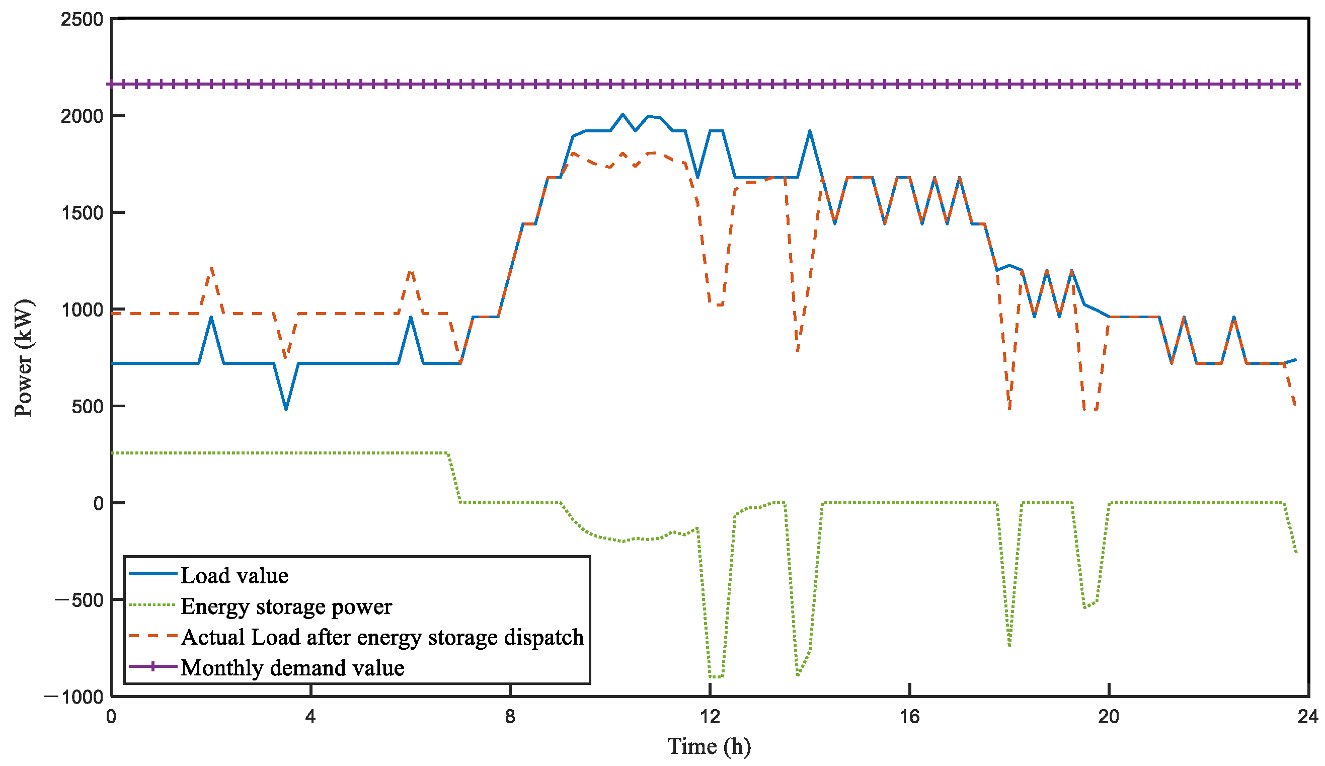
7.3.2. Daily Scheduling Results
Based on the monthly maximum demand determined by the pre-month optimization model, the daily optimization model in Section 4.2 is further adopted for daily energy storage scheduling based on the load curve of any day in December 2020, and the typical day is 24 December 2020. Figure 6 shows the forecast load and actual load power curve. Figure 7 shows the comparison curve of energy storage power between day-ahead optimization and intra-day optimization. Figure 8 shows the results of day-ahead scheduling optimization. Figure 9 shows the results of intra-day scheduling optimization. Figure 10 shows the comparison results of SOC for day-ahead optimization and intra-day optimization of energy storage.
It can be seen from Figure 6 that the load forecast curve and the actual load curve have basically the same changing trend. However, the actual load curve has large power fluctuations, and there are many valleys and peaks, while the power change of the load forecast curve is relatively stable. This difference is caused by load forecast errors and is difficult to avoid.
In order to illustrate the effectiveness of the intra-day rolling optimization scheduling strategy, Figure 7 compares the output curves of energy storage under the two optimization methods of day-ahead and intra-day. It can be seen that during the low electricity price period (0:00–7:00) of the two optimized operation methods, the energy storage is uniformly charged, and the “low storage and high discharge” arbitrage is used to improve the economic benefits of users. However, due to the existence of day-ahead load forecast errors, the energy storage curve in the discharge phase is quite different. Due to the continuous update of the rolling optimization model, there are multiple discharges in the energy storage during the optimization operation in the day, which is more in line with the volatility of the load power under actual conditions, and avoids the occurrence of no electricity to be discharged due to excessive discharge of energy storage, and improves the utilization rate of energy storage to a certain extent.
The rolling optimization of the daily operation of energy storage determines the charging and discharging power of the energy storage based on the load forecast data and the latest feedback actual load data, under the premise of meeting the system constraints, with the goal of maximizing the daily income. But only the energy storage plan value for the first time interval is executed. This is repeated over time until the energy storage completes the day’s scheduling. The optimization result is shown in Figure 9; it can be seen that the energy storage output can quickly respond to actual load power fluctuations during daily operation, and the coordination ability of the entire user system is further strengthened, making it easier to reach a balanced state. The rolling optimization strategy running within the day can dynamically respond to load forecast errors, effectively cut peaks and fill valleys for user systems, and reduce peak load.
Due to the error of the day-ahead load forecast, when the system adopts the results of the day-ahead optimization model of the energy storage, there is a power imbalance in actual operation, which causes a great burden on the large power grid. The rolling optimization strategy of energy storage intra-day operation updates the system status to the latest after each system operation, and performs feedback correction on the system, which can smooth power fluctuations and improve the robustness and accuracy of system operation optimization scheduling.
Comparing Figure 8 and Figure 9, it can be seen that the energy storage operation under the rolling optimization strategy of intra-day operation is more reasonable, and energy storage has different levels of output during the two peak electricity price periods. However, under the day-ahead optimization scheduling method, the energy storage has been completely discharged during the first peak electricity price period, resulting in no electricity to be discharged when the discharge is required at the subsequent peak time. This can also be seen in the SOC comparison results of the day-ahead operation and intra-day operation of energy storage in Figure 10.
It can be seen from Table 7 that during the day-ahead optimization operation, the saved electricity bill income for the day is USD 152.25; during the intra-day optimization operation, the saved electricity bill income for the day is USD 158.71. It can be found that, on the basis of meeting the maximum monthly demand, the intra-day optimized operation strategy is USD 6.45 more than the day-ahead optimized operation method in terms of peak-shaving and valley-filling revenue on this scheduling day, and the revenue has increased by 4.24%. It can be seen that the intra-day optimization operation strategy proposed in this paper can generate more considerable benefits on the basis of not exceeding the maximum monthly demand. The reason is that the day-ahead optimization operation method is a full-time offline optimization based on the load day-ahead forecast data. Load forecasting has errors; the errors accumulate over time during scheduling. The model accuracy is not high. In the actual operation process, the large power grid can smooth the error, which will generate more power purchase costs. The intra-day optimization operation strategy is based on the partial scheduling results of the day-ahead optimization operation method, taking into account the error of the load forecast data, the actual load data is fed back to the model in real time, forming a closed loop and continuously rolling forward optimization. The impact of load forecast errors on system scheduling is reduced, and the economy and reliability of user-side energy storage scheduling are improved.
8. Conclusions
Taking user-side energy storage as the research object, the paper considers demand response to establish an energy storage configuration optimization model, and proposes a rolling optimization scheduling strategy based on MPC for online energy management. The conclusions are as follows:
- (1)
- The established model comprehensively considers the cost models, such as energy storage installation cost, operation and maintenance cost, capacity attenuation cost, regularization function for smoothing the power fluctuation of the grid connection point, and the revenue models, such as electricity tariff revenue, reduced transformer cost due to peak load reduction, recovery value, demand response benefit, reliability benefit due to reduced power outages and government subsidy benefit. The refinement of the model in the planning stage has greatly improved the accuracy of energy storage configuration, which is closer to the actual project.
- (2)
- After the user participates in the power demand response, the energy storage will be discharged in a large amount during the agreed time period, and the charging and discharging activities will be carried out according to the “low storage and high discharge” during the rest of the time period. The configured energy storage achieves peak shaving and valley filling and reduction of load peaks, creating economic benefits for users and ensuring the safe and reliable operation of the power grid.
- (3)
- The proposed optimal scheduling strategy, from full-time offline optimization to partial real-time optimization, not only ensures the economic benefits of users, but also improves the accuracy of energy storage optimization scheduling. It is robust in an uncertain load forecasting environment.
- (4)
- The characteristics of MPC rolling optimization and feedback correction make the model constantly updated, and there may be no optimal solution. In order to make the optimization go forward in a normal and orderly manner, the load forecast data are used at the moment before the scheduling time, and the actual load data are not replaced, which ensures the feasibility of the optimized scheduling model.
In the transmission system, the grid power, load power and energy storage power are collected in real time through the power meter, and these data are returned to the control system. Through the proposed model, the scheduling plan is calculated in a few seconds and the scheduling command is able to be sent to the energy storage system for implementation. However, this may lead to some problems. For example, the actual load value may suddenly be too large or too small due to disturbances in the system or errors in the measured load data. This load value is fed back to the terminal control system, which calculates it as normal data. It will affect the performance of the energy storage scheduling model. This will be our next step of research.
Author Contributions
Conceptualization, Y.L., Q.L. and X.L.; formal analysis, X.L. and H.S.; investigation, Y.G.; methodology, Y.L. and Q.L.; software, H.G.; validation, Q.L., H.G. and D.B.; writing—review and editing, Y.L. and H.S. All authors have read and agreed to the published version of the manuscript.
Funding
This research was funded by National Natural Science Foundation of China (NSFC), grant number 52107175, and partly by Fundamental Research Funds for the Central Universities, grant number KG16076201.
Institutional Review Board Statement
Not applicable.
Informed Consent Statement
Not applicable.
Data Availability Statement
Not applicable.
Conflicts of Interest
The authors declare no conflict of interest.
References
- Tang, W.B.; Xiao, L.Y.; Shi, L.M.; Wang, Z.; Yang, W.H.; Wei, T.Z.; Du, X.J. Research on the principle and structure of a new energy storage technology named vacuum pipeline maglev energy storage. IEEE Access 2020, 8, 89351–89366. [Google Scholar] [CrossRef]
- Xiong, Y.F.; Si, Y.; Zheng, T.W.; Chen, L.J.; Mei, S.W. Optimal configuration of hydrogen storage in industrial park integrated energy system based on stackelberg game. Trans. China Electrotech. Soc. 2021, 36, 507–516. [Google Scholar]
- Li, Q.; Zhao, S.D.; Pu, Y.C.; Chen, W.R.; Yu, J. Capacity optimization of hybrid energy storage microgrid considering electricity-hydrogen coupling. Trans. China Electrotech. Soc. 2021, 36, 486–495. [Google Scholar]
- Zeng, B.; Xu, F.Q.; Liu, Y.X.; Liu, Y.; Gong, D.W. High-dimensional multi-objective optimization for multi-energy coupled system planning with consideration of economic, environmental and social factors. Trans. China Electrotech. Soc. 2021, 36, 1434–1445. [Google Scholar]
- Zheng, H.; Xie, L.R.; Ye, L.; Lu, P.; Wang, K.F. Hybrid energy storage smoothing output fluctuation strategy considering photovoltaic dual evaluation indicators. Trans. China Electrotech. Soc. 2021, 36, 1805–1817. [Google Scholar]
- Li, J.H.; Hou, T.; Mu, G.; Yan, G.G.; Li, C.P. Optimal control strategy for energy storage considering wind farm scheduling plan and modulation frequency limitation under electricity market environment. Trans. China Electrotech. Soc. 2021, 36, 1791–1804. [Google Scholar]
- Vatani, B.; Chowdhury, B.; Lin, J. The role of demand response as an alternative transmission expansion solution in a capacity market. IEEE Trans. Ind. Appl. 2018, 54, 1039–1046. [Google Scholar] [CrossRef]
- Xiang, B.; Li, K.P.; Ge, X.X.; Zhen, Z.; Lu, X.X.; Wang, F. Day-ahead probabilistic forecasting of smart households’ demand response capacity under incentive-based demand response program. In Proceedings of the 2019 IEEE Sustainable Power and Energy Conference (iSPEC), Beijing, China, 21–23 November 2019. [Google Scholar]
- Byers, C.; Levin, T.; Botterud, A. Capacity market design and renewable energy: Performance incentives, qualifying capacity, and demand curves. Electron. J. 2018, 31, 65–74. [Google Scholar] [CrossRef]
- Sugimura, M.; Senjyu, T.; Krishna, N.; Mandal, P.; Abdel-Akher, M.; Hemeida, A.M. Sizing and operation optimization for renewable energy facilities with demand response in micro-grid. In Proceedings of the 2019 20th International Conference on Intelligent System Application to Power Systems (ISAP), New Delhi, India, 10–14 December 2019. [Google Scholar]
- Xue, J.H.; Ye, J.L.; Tao, Q.; Wang, D.S.; Sang, B.Y.; Yang, B. Economic feasibility of user-side battery energy storage based on whole-life-cycle cost model. Power Syst. Technol. 2016, 40, 2471–2476. [Google Scholar]
- Jia, X.C.; Li, X.J.; Wang, H.L.; Zhang, Y.H.; Hui, D. Research on consistency assessment method for energy storage battery based on operating data fusion. Distrib. Util. 2017, 34, 29–35. [Google Scholar]
- Yan, P.; Wang, K.; He, K. Study on optimal configuration scheme of user-side battery energy storage system. Electron. Energy Manag. Technol. 2020, 590, 67–71. [Google Scholar]
- Xiong, X.; Ye, L.; Yang, R.G. Optimal allocation and economic benefits analysis of energy storage system on power demand side. Autom. Electron. Power Syst. 2015, 39, 42–48+88. [Google Scholar]
- Xiong, X.; Yang, R.G.; Ye, L.; Li, J.L. Economic evaluation of large-scale energy storage allocation in power demand side. Trans. China Electrotech. Soc. 2013, 28, 224–230. [Google Scholar]
- Ding, Y.X.; Xu, Q.S.; Lv, Y.J.; Li, L. Optimal configuration of user-side energy storage considering power demand management. Power Syst. Technol. 2019, 43, 1179–1186. [Google Scholar]
- Zhao, Y.T.; Wang, H.F.; He, B.T.; Xu, W.N. Optimization strategy of configuration and operation for user-side battery energy storage. Autom. Electron. Power Syst. 2020, 44, 121–128. [Google Scholar]
- Ma, X.F.; Chen, J.; Yu, S.Y.; Li, S.Y.; Lu, W.B. Research on user side energy storage optimization configuration considering capacity market. Trans. China Electrotech. Soc. 2020, 35, 4028–4037. [Google Scholar]
- Zhang, J.Y.; Chen, H.Y.; Wang, W.H. Research on optimal configuration strategy of user-side energy storage considering demand management. Power Demand Side Manag. 2020, 22, 19–24+37. [Google Scholar]
- Chen, L.J.; Wu, T.T.; Liu, H.B.; Huang, G.Y.; Xu, X.H. Demand management based two-stage optimal storage model for large users. Autom. Electron. Power Syst. 2019, 43, 194–200. [Google Scholar]
- Lin, J.H.; Gu, X.W.; Ma, L. Optimal sizing and control of demand-side battery energy storage system. Energy Storage Sci. Technol. 2018, 7, 90–99. [Google Scholar]
- Guo, J.Y.; Liu, Y.; Guo, Y.L.; Xu, L.X. Configuration evaluation and operation optimization model of energy storage in different typical user-side. Power Syst. Technol. 2020, 44, 4245–4254. [Google Scholar]
- Pan, F.R.; Zhang, J.Y.; Zhou, Z.W.; Zhang, X.; Zheng, X.C. Cost-benefit and investment risk analysis of user-side battery energy storage system. Zhejiang Electron. Power 2019, 38, 43–49. [Google Scholar]
- Wang, Z.Y.; Yi, Z.K.; Zhou, J.G.; Duan, R.H.; Zhu, T.; Xia, T.; Xu, Y.L. Wind power integration capability evaluation of large-scale combined heat and power system with additional heat source. In Proceedings of the 2019 IEEE PES Asia-Pacific Power and Energy Engineering Conference (APPEEC), Macao, China, 1–4 December 2019. [Google Scholar]
- Deng, B.F.; Fang, J.K.; Hui, Q.; Zhang, T.Y.; Chen, Z.; Teng, Y.; Xi, X. Optimal scheduling for combined district heating and power systems using subsidy strategies. CSEE J. Power Energy Syst. 2019, 5, 399–408. [Google Scholar]
- Chen, Z.Y.; Wang, D.; Jia, H.J.; Wang, W.L.; Guo, B.Q.; Qu, B.; Fan, M.H. Research on optimal day-ahead economic dispatching strategy for microgrid considering P2G and multi-source energy storage system. Proc. CSEE 2017, 37, 3067–3077. [Google Scholar]
- Ma, T.F.; Wu, J.Y.; Hao, L.L. Energy flow modeling and optimal operation analysis of micro energy grid based on energy hub. Energy Convers. Manag. 2017, 133, 292–306. [Google Scholar] [CrossRef]
- Moghaddam, I.G.; Saniei, M.; Mashhour, E. A comprehensive model for self-scheduling an energy hub to supply cooling, heating and electrical demands of a building. Energy 2016, 94, 157–170. [Google Scholar] [CrossRef]
- Jin, X.L.; Mu, Y.F.; Jia, H.J.; Yu, X.D.; Chen, N.S.; Ge, X.J.; Yu, J.C. Optimal scheduling method for a combined cooling, heating and power building microgrid considering virtual storage system at demand side. Proc. CSEE 2017, 37, 581–590. [Google Scholar]
- Zhu, X.R.; Xie, W.Y.; Lu, G.W. Day-ahead scheduling of combined heating and power microgrid with the interval multi-objective linear programming. High. Volt. Eng. 2021, 47, 2668–2679. [Google Scholar]
- Qiu, Z.; Wang, B.B.; Ben, S.J.; Hu, N. Bi-level optimal configuration planning model of regional integrated energy system considering uncertainties. Electron. Power Autom. Equip. 2019, 39, 176–185. [Google Scholar]
- Huang, Z.H.; Zhang, Y.C.; Zheng, F.; Lin, J.H.; An, X.L.; Shi, H. Day-ahead and real-time energy management method for active distribution networks based on coordinated optimization of different stakeholders. Power Syst. Technol. 2021, 45, 2299–2308. [Google Scholar]
- Zhu, L.; Li, X.J.; Tang, L.J.; Tian, Z.Q.; Cui, K.S. Distributionally robust optimal operation for microgrid considering phase change storage and building storage. Power Syst. Technol. 2021, 45, 2308–2319. [Google Scholar]
- Sang, B.; Zhang, T.; Liu, Y.J.; Chen, Y.D.; Liu, L.S.; Wang, R. Energy management system research of multi-microgrid: A review. Proc. CSEE 2020, 40, 3077–3093. [Google Scholar]
- Sun, H.J.; Zhang, L.L.; Peng, C.H. Time-domain rolling optimal scheduling of microgrid based on differential demand response model predictive control. Power Syst. Technol. 2021, 45, 3096–3105. [Google Scholar]
- Yang, M.T.; Zhou, B.X.; Dong, S.; Lin, N.; Li, Z.G.; He, F.Y. Design and dispatch optimization of microgrid electricity market supported by blockchain. Electron. Power Autom. Equip. 2019, 39, 155–161. [Google Scholar]
- Jin, X.L.; Mu, Y.F.; Jia, H.J.; Yu, X.D.; Xu, K.; Xu, J. Model predictive control based multiple-time-scheduling method for microgrid system with smart buildings intergrated. Autom. Electron. Power Syst. 2019, 43, 25–33. [Google Scholar]
- Zhou, X.Q.; Ai, Q.; Wang, H. Distributed optimal scheduling of microgrid cluster with function of plug and play. Autom. Electron. Power Syst. 2018, 42, 106–113. [Google Scholar]
- Zhang, F.X.; Jin, X.L.; Mu, Y.F.; Jia, H.J.; Yu, X.D.; Liu, D.T. Model predictive scheduling method for a building microgrid considering virtual storage system. Proc. CSEE 2018, 38, 4420–4428+4642. [Google Scholar]
- Wang, C.S.; Lv, C.X.; Li, P.; Li, S.Q.; Zhao, K.P. Multiple time-scale optimal scheduling of community integrated energy system based on model predictive control. Proc. CSEE 2019, 39, 6791–6803+7093. [Google Scholar]
- Zhang, H.; Zhang, J.; Xiao, Y.Q.; He, Y.; Liu, Y.; Fan, L.Q. Research on intra-day hierarchical dispatching of microgrid based on model prediction. Electron. Power Sci. Eng. 2021, 37, 1–10. [Google Scholar]
- Domanski, P.D.; Lawrynczuk, M. Impact of MPC embedded performance index on control quality. IEEE Access 2021, 9, 24787–24795. [Google Scholar] [CrossRef]
- Soloperto, R.; Kohler, J.; Allgower, F. Augmenting MPC schemes with active learning: Intuitive tuning and guaranteed performance. IEEE Control. Syst. Lett. 2020, 4, 713–718. [Google Scholar] [CrossRef]
- Liu, Q.Q.; Liu, Y.S.; Wen, Y.T.; He, J.; Li, X.; Bi, D.Q. Short-term load forecasting method based on PCC-LSTM model. J. Beijing Univ. Aeronaut. Astronaut. 2021, 30, 1–11. [Google Scholar]
Figure 1.
Schematic diagram of MPC principle.

Figure 2.
Flow chart of intra-day optimized scheduling strategy for energy storage.

Figure 3.
Flow chart of energy storage solution.

Figure 4.
Curve of load power.

Figure 5.
The change curve of average annual net income of users with energy storage capacity and power.
Figure 5.
The change curve of average annual net income of users with energy storage capacity and power.

Figure 6.
Load curve on 24 December 2020.

Figure 7.
Energy storage power change curve on 24 December 2020.

Figure 8.
Day-ahead optimized scheduling results of energy storage on 24 December 2020.

Figure 9.
Intra-day optimized scheduling results of energy storage on 24 December 2020.

Figure 10.
SOC comparison results of energy storage operation on 24 December 2020.


Table 1.
Related parameters of energy storage battery.
| Parameters | Lithium Iron Phosphate Battery | Lead Carbon Battery | Sodium Sulfur Battery |
|---|---|---|---|
| (USD/(kWh)) | 313.80 | 101.99 | 219.66 |
| (USD/(kW)) | 175.73 | 188.28 | 65.90 |
| (USD/(kW·a)) | 15.22 | 3.92 | 19.46 |
| 0.90 | 0.88 | 0.75 | |
| Depth of discharge, dod | 0.9 | 0.7 | 0.6 |
| State of charge, SOC | [0.2,0.8] | [0.3,0.8] | [0.4,0.8] |
| Daily cycles, n | 1 | 1 | 1 |
| Discount rate, r (%) | 6 | 6 | 6 |
Table 2.
Transformer related parameters.
| Parameters | Values |
|---|---|
| Ratio of installation cost to equipment cost, α | 0.30 |
| (USD/(kV·A)) | 78.45 |
| Load factor, K | 0.75 |
| 0.85 |
Table 3.
Peak-to-valley time-of-use electricity prices for large industries in the suburbs of Beijing.
Table 3.
Peak-to-valley time-of-use electricity prices for large industries in the suburbs of Beijing.
| Time Period | Time | Electricity Price (USD/(kWh)) |
|---|---|---|
| Valley | 0:00–7:00 | 0.05087 |
| Peak | 10:00–15:00, 18:00–21:00 | 0.14650 |
| Flat | 7:00–10:00, 15:00–18:00, 21:00–24:00 | 0.09800 |
Table 4.
Energy storage configuration results.
| Parameters | Lithium Iron Phosphate Battery | Lead Carbon Battery | Sodium Sulfur Battery |
|---|---|---|---|
| Equivalent operating life, T (a) | 17 | 10 | 12 |
| Rated capacity, (kWh) | 2694 | 3660 | 3368 |
| (kW) | 900 | 1108 | 1796 |
| (day) | 252 | 252 | 252 |
| 0.1 | 0.1 | 0.1 |
Table 5.
Costs and benefits of energy storage configuration.
| Project | Lithium Iron Phosphate Battery | Lead Carbon Battery | Sodium Sulfur Battery |
|---|---|---|---|
| Average annual investment cost (USD 10,000) | 15.4876 | 12.8548 | 18.2082 |
| Average annual net benefit (USD 10,000) | 15.5205 | 19.4179 | 14.6262 |
| Average annual total benefit (USD 10,000) | 31.0081 | 32.2728 | 32.8345 |
| Annual average basic electricity bill benefit (USD 10,000) | 5.7331 | 6.3450 | 7.1029 |
| Annual average electricity cost benefit (USD 10,000) | 3.8597 | 4.2520 | 3.1898 |
| Annual average transformer cost benefit reduced by peak load reduction (USD 10,000) | 14.3971 | 14.3971 | 14.3971 |
| Annual average capacity market benefit (USD 10,000) | 5.8885 | 5.8885 | 5.8885 |
| Annual average reliability benefit (USD 10,000) | 1.1297 | 1.3901 | 2.2547 |
| Total investment cost (USD 10,000) | 263.2892 | 128.5482 | 218.4942 |
| Payback period (year) | 8.5 | 4.0 | 6.7 |
| Cost performance index | 2.0 | 2.5 | 1.8 |
| Net benefit in the whole life cycle (USD 10,000) | 263.8415 | 194.1732 | 175.5146 |
| Total benefit in the whole life cycle (USD 10,000) | 527.1369 | 322.7213 | 394.0088 |
| Return on investment (%) | 100 | 151 | 80 |
Table 6.
Pre-month optimization results in December 2020.
| Parameters | Values |
|---|---|
| Maximum demand for forecast data (kW) | 2700 |
| Maximum reported demand (kW) | 2161 |
| Electricity bill benefit (USD) | 3844.05 |
| Basic electricity bill benefit (USD) | 4063.71 |
| Monthly net benefit (USD) | 7892.07 |
Table 7.
Daily scheduling operation results of energy storage.
| Parameters | Day-Ahead Optimization Operation | Intra-Day Optimization Operation |
|---|---|---|
| Daily electricity fee benefit (USD) | 152.26 | 158.71 |
| Input data peak (kW) | 2006 | 2160 |
| Peak load after energy storage scheduling (kW) | 1805 | 1805 |
Publisher’s Note: MDPI stays neutral with regard to jurisdictional claims in published maps and institutional affiliations. |
© 2021 by the authors. Licensee MDPI, Basel, Switzerland. This article is an open access article distributed under the terms and conditions of the Creative Commons Attribution (CC BY) license (https://creativecommons.org/licenses/by/4.0/).
Share and Cite
MDPI and ACS Style
Liu, Y.; Liu, Q.; Guan, H.; Li, X.; Bi, D.; Guo, Y.; Sun, H. Optimization Strategy of Configuration and Scheduling for User-Side Energy Storage. Electronics 2022, 11, 120. https://doi.org/10.3390/electronics11010120
AMA Style
Liu Y, Liu Q, Guan H, Li X, Bi D, Guo Y, Sun H. Optimization Strategy of Configuration and Scheduling for User-Side Energy Storage. Electronics. 2022; 11(1):120. https://doi.org/10.3390/electronics11010120
Chicago/Turabian StyleLiu, Yushan, Qianqian Liu, Huaimin Guan, Xiao Li, Daqiang Bi, Yingjun Guo, and Hexu Sun. 2022. "Optimization Strategy of Configuration and Scheduling for User-Side Energy Storage" Electronics 11, no. 1: 120. https://doi.org/10.3390/electronics11010120
Note that from the first issue of 2016, this journal uses article numbers instead of page numbers. See further details here.