
Optimization of Different Deployments and Resolution of Antenna Arrays in SWIPT


1
Department of Electrical and Computer and Engineering Department, Tamkang University, New Taipei City 251301, Taiwan
2
Department of Computer Information and Network Engineering, Lunghwa University of Science and Technology, Taoyuan City 333326, Taiwan
3
Department of Electrical and Electronic, University Tunku Abdul Rahman, Kajang 43200, Malaysia
*
Author to whom correspondence should be addressed.
Electronics 2022, 11(1), 19; https://doi.org/10.3390/electronics11010019
Submission received: 4 November 2021
/
Revised: 19 December 2021
/
Accepted: 21 December 2021
/
Published: 22 December 2021
(This article belongs to the Special Issue Electronic Devices on Intelligent IoT Applications)
Abstract
:In this paper, three different deployment antenna arrays with circular, triangular and rectangular shapes were used to optimize the simultaneous wireless information and power transfer (SWIPT) system for the Internet of Things (IoT). Ray-tracing was employed to channel the model for a real environment. Self-adaptive dynamic differential evolution (SADDE) was used to optimize the harvesting power ratio with bit error rate constrained by the two different resolutions of feed length (high resolution and low resolution). Numerical results show that those three antenna arrays can achieve the goal for information quality in both resolutions. The harvesting power ratio for the circular array is the best and the harvesting power ratio for the rectangular array is the worst. The harvesting power ratio for the low-resolution case is 25% lower than the high-resolution case. However, the circular antenna array is the best deployment in those three different arrays for both high and low resolutions.
1. Introduction
Millimeter wave (mm-Wave) communication is very promising in terms of high data rate and it is being studied as a key 5G technology to accommodate the expansion of the Internet of Things (IoT) [1,2,3,4,5,6,7]. Because of their smaller wavelength, massive antennas can be deployed in the limited space at the mm-Wave. Nevertheless, this does cause serious path loss and shadow fading at mm-Wave. The technique of beamforming by antenna array was used to solve those problems at the mm-Wave in recent years. In IEEE 802.11ad, the codebook was set in the protocol for quick pairing and eventually it was extended to a 5G technology application. In addition to the fixed pattern of the codebook, it can also be adjusted by the algorithm for beamforming according to the environment [8,9].
In IoT applications, numerous smart devices were deployed in mm-Wave worldwide for wireless communication. Among them, some devices use low-power design and power harvesting is considered as a solution for providing a perpetual and effective energy supply. As a result, the wireless powered transfer (WPT) and the simultaneous wireless information and power transfer (SWIPT) have been widely investigated in recent years [10,11,12,13,14,15,16,17,18]. In [19], the coverage analysis for energy-harvesting by unmanned aerial vehicle cellular networks at millimeter-wave communication was investigated. The authors in [20] developed a framework to study the security, reliability and energy coverage performance of downlink mm-Wave simultaneous wireless information and power transfer unmanned aerial vehicle (UAV) networks. In [21], the authors used the Nakagami fading channel to analyze energy harvesting performance in low-power devices powered by a mm-Wave cellular network. The problem of hybrid beamforming designed with the low-resolution phase shifter was investigated in [22]. In ref. [23], the optimal analytic solution with the signal-to-interference plus noise ratio (SINR) constraint was presented for narrow band signal. The authors in [24] addressed the energy efficiency (EE) optimization problem for the SWIPT multiple-input–multiple-output broadcast channel.
However, most papers have only dealt with the optimal analytic solution with some constraints for the narrow band signal and considered the stochastic channel in their analysis. Different adjustments in terms of feed length and the deployment of different antenna array shapes have not yet been simultaneously investigated in the literature with regard to SWIPT systems. In this paper, three different wide-band antenna arrays with variable resolutions were used to generate the array pattern for some simple IoT sensors. We optimized the power harvesting efficiency under the constraint of the BER by self-adaptive dynamic differential evolution (SADDE).
The system model and the deployment of antenna arrays are presented in Section 2. Section 3 explains the SADDE and the objective function. In Section 4, numerical results for three different deployment cases with high resolution and low-resolution feed length by evolution algorithm are presented. The system quality and harvesting power are compared. Conclusions are given in Section 5.
2. System Model
For the environment channel model, the ray-tracing method was used to compute the path loss and environment effect at the mm-Wave communication. The frequency response can be expressed as
where N is the number of the total path, f is the frequency, i is the path index of the ray. is the i-th receiving magnitude which includes the intensity and the phase information. is the phase shift according to the time delay with the contribution of frequency. The time domain impulse response of the equivalent baseband can be obtained by the inverse Fourier transform and can be expressed as follows:
where h(t) is the impulse response. For the SWIPT system, the power-splitting with the splitting ratio 0.5 is used. The architecture is shown in Figure 1. Here, the energy harvester and information decoder are behind the energy splitter.
The wireless harvested power is modeled as
where η is the portion of RF signals utilized for power gathering. The information decoder quality BER is used to investigate the inter-symbol-interference in our SWIPT system and it is computed as the following formula [8,9]:
where is the complementary error function and is the binary sequence.
The array factor is used to compute the array equivalent pattern and the relationship of the coordinate is shown in Figure 2.
According to Figure 2, we can express the array factor as
where polar angle and azimuthal angle are the spherical coordinates system. a is the distance from the origin to the antenna position. and are the spherical coordinates of the transmitting antenna. M is the total number of antennas in the antenna array. k is the wavenumber ( is the wavelength). The adjustment of the phase delay and antenna power can be expressed as
where and are the excitation current and the phase delay, respectively. The relation between feed length and can be expressed as
where is the relative permittivity of the feed line and is the feed length of the transmission line which can be used to adjust the phase delay. c is the light speed.
3. Evolution Algorithm
SADDE was developed from the dynamic differential evolution (DDE) [25]. This added some mechanism to dynamically change the adjustment factor during the search. Figure 3 shows the SADDE algorithm flowchart.
- Step 1. In the first step, we randomly initiate the parameter of the population for the antenna array. There are d dimensional adjustment parameters in each population.
- Step 2. According to the p-th population’s parameters, calculate the objective function value and update the best value of the population.
- Step 3. Mutate the trial vector based on the control vector and adjust the control vector for the next generation.
- Step 4. By the presetting probability, decide whether the crossover mechanism is needed to start. If starting the mechanism, we compare the crossover objective value with the former objective value.Step 5. Update the position of the global best population.
- Step 6. According to the total number of populations and the number of generations, go to step 2 or stop operating the algorithm.
In order to handle two different requirements at the same time, we designed two objectives for optimization by algorithms and we should solve the unit inconsistent problem. One objective is the BER and the other is the total harvesting power. Since the BER usually have a minimum quality requirement, we can divide the minimum limitation of BER by the required BER to solve the inconsistency of the unit. The different objective can be optimized into one objective function. The with the BER constrained condition of is defined as
The total power harvesting can be expressed as
where is the total number of receivers in the environment. The multiple objective function is:
4. Numerical Results
The office environment is shown in Figure 4. We take the mm-Wave system of frequencies ranging from 39 to 40 GHz and used the ray tracing technique to compute the environment channel. There are three receivers (Rx1, Rx2, Rx3) and one transmitter (Tx) in the office. We then consider two kinds of nodes for SWIPT and WPT. The Rx1 uses 50% power-splitting for information decoding and harvests the half power with 60% power efficiency. The WPT nodes Rx2 and Rx3 can harvest 100% power at 60% power efficiency. The transmitter uses three different deployments as shown in Figure 5. Each antenna array has three layers with a vertical distance of λ/2. Additionally, each layer has 16 antennas. The unit of the antenna uses the wideband dipole antenna with a λ/2 distance separated at least. In other words, there are 48 antennas for each deployment. The transmission power to the noise at receiver (SNR_T) is set to 33 dB. For the feed length adjustment, we use SADDE to optimize the objective function and set the total iteration to 500. The population size is 60 and the adjustment parameter is 48 for each antenna array. Note that the low resolution of feed lengths only has four phases with 0o, 90o, 180o, 270o.
Figure 6 shows the total harvesting power ratio by high resolution feed length for different deployments. The harvesting power ratio is based on the harvesting power under the zero phase of a circular array. It can be seen that the circular array has the best harvesting power ratio and the convergence speed. The harvesting power ratio for the triangular deployment is better than that for the rectangular deployment. However, the convergence speed of the triangular deployment is the slowest. For the low-resolution feed length, the harvesting power ratio for the circular, triangular and rectangular antenna array is shown in Figure 7. Compared to the high resolution, the harvesting power ratios are all decreased by approximately 30% and have a slow convergence speed for all three different deployments. Then, we compare the criterion for BER. In Figure 8, we can see that the BER constraint for high-resolution feed length adjustment is satisfied no matter what the deployments are. It can be seen that the BER and harvesting power are both almost converged after 400 iterations. In the low resolution, as shown in Figure 9, it seems that the optimization for the BER is still good. According to the results, it is clear that the objective function shown in Equation (10) is useful for different layouts of the antenna array. Additionally, it does prove that the different deployments do affect the final harvesting power ratio.
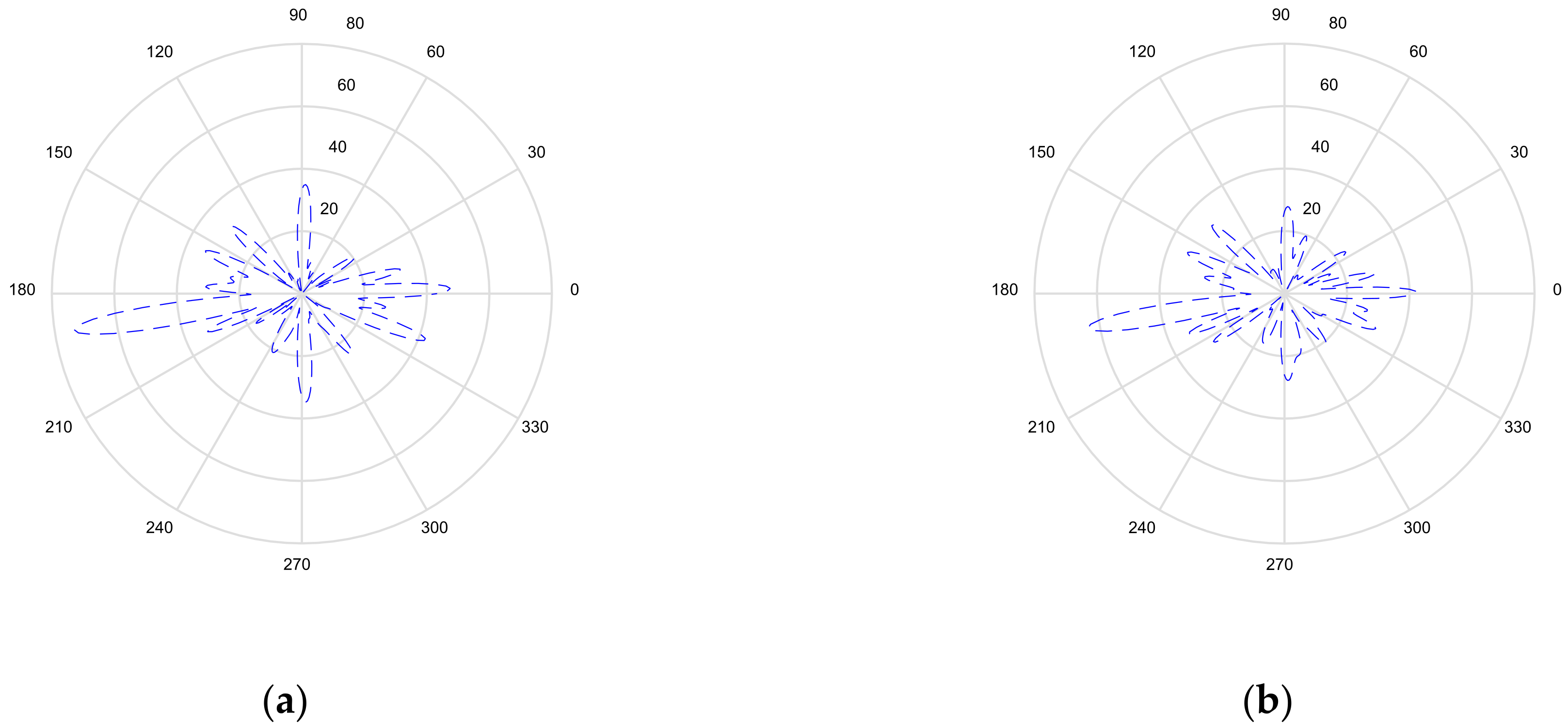
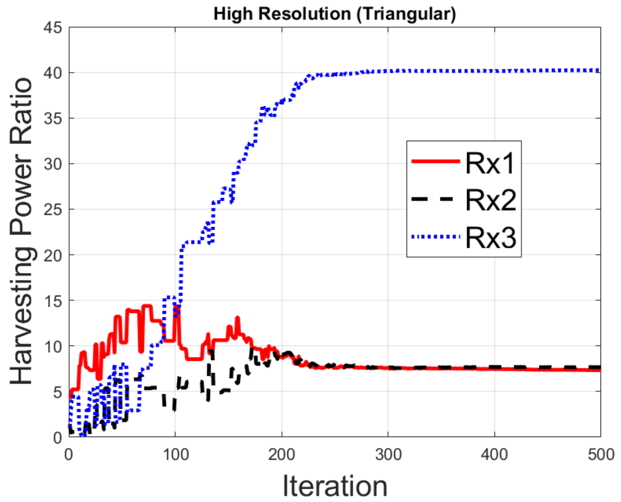
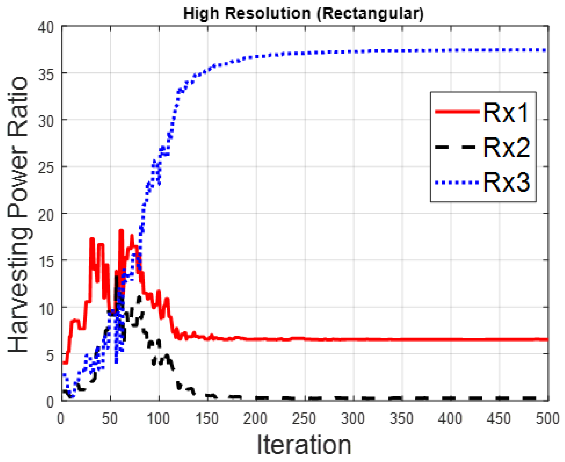
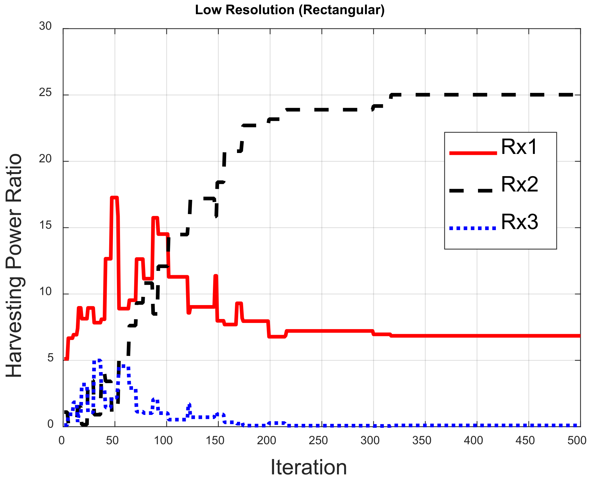
Figure 10 illustrates the optimized pattern with different resolutions for the circular array. Figure 10a shows the pattern focused on Rx1, Rx2 and Rx3 for the high-resolution case—where the gain for Rx3 is the largest and the gain for Rx1 is smallest. This is because Rx3 is closest to the transmitter in the environment and Rx1 has split the power for SWIPT. The pattern gains are similar at the three receivers in Figure 10b for the low-resolution case. It can be seen that the harvesting power with low resolution is less than with high resolution. Figure 11 displays the pattern for the triangular array. The pattern can be focused on three receivers, as shown in Figure 10, but the total harvesting power ratio is less than that for the circular array. The optimized pattern for the rectangular array is depicted in Figure 12. Figure 12a shows that the pattern cannot simultaneously be focused on three receivers—even in the high-resolution case. The rectangular deployment has the worst harvesting power ratio, though it does reach the BER constraint. For the low-resolution case, optimization has found the local solution instead of the global solution, as shown in Figure 12b, in which the pattern is focused on Rx2. Note that Rx3 is close to the transmitter. As a result, the pattern is not the best solution. Figure 13, Figure 14, Figure 15, Figure 16, Figure 17 and Figure 18 are the harvesting power ratios at Rx1, Rx2 and Rx3 for the circular, triangular and rectangular with the high- and low-resolution cases, respectively. By comparing Figure 13, Figure 14 and Figure 15, the harvesting power of Rx3 is the largest for the three arrays. Moreover, the harvesting power of Rx2 for the circular array is larger than those of the other two arrays. The circular array and the triangular array can be focused on three receivers. However, the rectangular array can only be focused on two receivers. From Figure 16, Figure 17 and Figure 18, we can see that the largest harvesting power ratio is Rx3 for the circular and triangular array. However, for the rectangular array, the worst harvesting power ratio is Rx3 while the largest harvesting power ratio is Rx2. In conclusion, the circular array and triangular array are more efficient than the rectangular array. From those numerical results, we can see that the deployment shapes can affect the adjustment and the low-resolution beamforming will increase difficulty in the optimization.
5. Conclusions
In this paper, we compared three different deployments and two different resolution adjustments to optimize the harvesting power and information quality for the SWIPT system at the mm-Wave in a real environment. We applied SADDE to optimize the three different deployments of the antenna array. In the SWIPT system, we not only used BER for information quality, but we also used the energy harvester for harvesting power. The high-resolution adjustment can converge faster than the low resolution, in addition to achieving better a harvesting power ratio. In addition, three antenna arrays can achieve the goal for information quality in both resolutions, but the harvesting power ratio may decrease by approximately 25% due to the difficulty of adjustment for the low-resolution case. Numerical results show that the circular array has the largest harvesting power ratio for both the high- and low-resolution cases. Thus, the circular antenna array is the best deployment in this environment due to its uniform characteristic deployment. Although the deployment shape and environment may affect the results, our proposed multiple objective function was proven to be good for SWIPT optimization.
Author Contributions
Conceptualization, C.-C.C. and E.H.L.; methodology, C.-C.C. and Y.-T.C.; software, Y.-T.C. and W.C.; validation, H.-Y.W.; formal analysis, C.-C.C.; investigation, H.-Y.W.; resources, W.C.; data curation, H.-Y.W.; writing—original draft preparation, C.-C.C. and Y.-T.C.; writing—review and editing, H.-Y.W.; visualization, H.-Y.W.; supervision, E.H.L.; project administration, H.-Y.W.; funding acquisition, H.-Y.W. All authors have read and agreed to the published version of the manuscript.
Funding
[Ministry of Science and Technology, Taiwan] [MOST 110-2221-E-032 -012 -].
Conflicts of Interest
The authors declare no conflict of interest.
References
- Ghosh, A.; Maeder, A.; Baker, M.; Chandramouli, D. 5G Evolution: A View on 5G Cellular Technology beyond 3GPP Release 15. IEEE Access 2019, 7, 127639–127651. [Google Scholar] [CrossRef]
- Agrawal, S.K.; Sharma, K. 5G millimeter wave (mmWave) communications. In Proceedings of the 2016 3rd International Conference on Computing for Sustainable Global Development (INDIACom), New Delhi, India, 16–18 March 2016; pp. 3630–3634. [Google Scholar]
- Ansari, R.I.; Chrysostomou, C.; Hassan, S.A.; Guizani, M.; Mumtaz, S.; Rodriguez, J.; Rodrigues, J.J. 5G D2D Networks: Techniques, Challenges, and Future Prospects. IEEE Syst. J. 2018, 12, 3970–3984. [Google Scholar] [CrossRef]
- Shafique, K.; Khawaja, B.A.; Sabir, F.; Qazi, S.; Mustaqim, M. Internet of Things (IoT) for Next-Generation Smart Systems: A Review of Current Challenges, Future Trends and Prospects for Emerging 5G-IoT Scenarios. IEEE Access 2020, 8, 23022–23040. [Google Scholar] [CrossRef]
- Zhou, B.; Liu, A.; Lau, V. Successive Localization and Beamforming in 5G mmWave MIMO Communication Systems. IEEE Trans. Signal Processing 2019, 67, 1620–1635. [Google Scholar] [CrossRef]
- Zhao, X.; Du, F.; Geng, S.; Sun, N.; Zhang, Y.; Fu, Z.; Wang, G. Neural network and GBSM based time-varying and stochastic channel modeling for 5G millimeter wave communications. China Commun. 2019, 16, 80–90. [Google Scholar] [CrossRef]
- Park, J.J.; Moon, J.H.; Lee, K.-Y.; Kim, D.I. Transmitter-Oriented Dual-Mode SWIPT with Deep-Learning-Based Adaptive Mode Switching for IoT Sensor Networks. IEEE Internet Things J. 2020, 7, 8979–8992. [Google Scholar] [CrossRef]
- Lai, G.D.; Chiu, C.C.; Cheng, Y.T. BER reduction for ultra wideband multicasting system by beamforming techniques. J. Appl. Sci. Eng. 2018, 21, 587–594. [Google Scholar]
- Chiu, C.C.; Chen, C.H.; Cheng, Y.T.; Lee, Y.L.; Chou, Y.K. Beamforming Techniques at Both Transmitter and Receiver for Indoor Wireless Communication. J. Appl. Sci. Eng. 2018, 21, 407–412. [Google Scholar]
- Zhang, J.; Zheng, G.; Krikidis, I.; Zhang, R. Fast specific absorption rate aware beamforming for downlink SWIPT via deep learning. IEEE Trans. Veh. Technol. 2020, 69, 16178–16182. [Google Scholar] [CrossRef]
- Lee, K.; Lee, W. Learning-Based Resource Management for SWIPT. IEEE Syst. J. 2020, 14, 4750–4753. [Google Scholar] [CrossRef]
- Zhang, Z.; Lu, Y.; Huang, Y.; Zhang, P. Neural Network-Based Relay Selection in Two-Way SWIPT-Enabled Cognitive Radio Networks. IEEE Trans. Veh. Technol. 2020, 69, 6264–6274. [Google Scholar] [CrossRef]
- Hu, Z.; Xie, D.; Jin, M.; Zhou, L.; Li, J. Relay Cooperative Beamforming Algorithm Based on Probabilistic Constraint in SWIPT Secrecy Networks. IEEE Access 2020, 8, 173999–174008. [Google Scholar] [CrossRef]
- Li, Q.; Yang, L. Robust Optimization for Energy Efficiency in MIMO Two-Way Relay Networks with SWIPT. IEEE Syst. J. 2020, 14, 196–207. [Google Scholar] [CrossRef]
- Liu, F.; Liu, Y.; Liu, Y.; Yu, J. Secure Beamforming in Full-Duplex Two-Way Relay Networks with SWIPT for Multimedia Transmission. IEEE Access 2020, 8, 26851–26862. [Google Scholar] [CrossRef]
- Luo, J.; Tang, J.; So, D.K.; Chen, G.; Cumanan, K.; Chambers, J.A. A Deep Learning-Based Approach to Power Minimization in Multi-Carrier NOMA with SWIPT. IEEE Access 2019, 7, 17450–17460. [Google Scholar] [CrossRef]
- Qi, Q.; Chen, X.; Ng, D.W.K. Robust Beamforming for NOMA-Based Cellular Massive IoT with SWIPT. IEEE Trans. Signal Processing 2020, 68, 211–224. [Google Scholar] [CrossRef]
- Sun, X.; Yang, W.; Cai, Y.; Wang, M. Secure mmWave UAV-Enabled SWIPT Networks Based on Random Frequency Diverse Arrays. IEEE Internet Things J. 2021, 8, 528–540. [Google Scholar] [CrossRef]
- Wang, X.; Gursoy, M.C. Coverage Analysis for Energy-Harvesting UAV-Assisted mmWave Cellular Networks. IEEE J. Sel. Areas Commun. 2019, 37, 2832–2850. [Google Scholar] [CrossRef] [Green Version]
- Sun, X.; Yang, W.; Cai, Y. Secure Communication in NOMA-Assisted Millimeter-Wave SWIPT UAV Networks. IEEE Internet Things J. 2020, 7, 1884–1897. [Google Scholar] [CrossRef]
- Khan, T.A.; Alkhateeb, A.; Heath, R.W. Millimeter Wave Energy Harvesting. IEEE Trans. Wirel. Commun. 2016, 15, 6048–6062. [Google Scholar] [CrossRef] [Green Version]
- Liu, R.; Li, H.; Guo, Y.; Li, M.; Liu, Q. Hybrid Beamformer Design with Low-Resolution Phase Shifters in MU-MISO SWIPT Systems. In Proceedings of the 2018 10th International Conference on Wireless Communications and Signal Processing (WCSP), Hangzhou, China, 18–20 October 2018; pp. 1–6. [Google Scholar]
- Hao, W.; Sun, G.; Chu, Z.; Xiao, P.; Zhu, Z.; Yang, S.; Tafazolli, R. Beamforming Design in SWIPT-Based Joint Multicast-Unicast mmWave Massive MIMO With Lens-Antenna Array. IEEE Wirel. Commun. Lett. 2019, 8, 1124–1128. [Google Scholar] [CrossRef]
- Tang, J.; So, D.K.C.; Zhao, N.; Shojaeifard, A.; Wong, K. Energy Efficiency Optimization with SWIPT in MIMO Broadcast Channels for Internet of Things. IEEE Internet Things J. 2018, 5, 2605–2619. [Google Scholar] [CrossRef] [Green Version]
- Chiu, C.C.; Tong, Y.X.; Cheng, Y.T. Comparison of SADDE and PSO for Smart Antennas in Wireless Communication. Int. J. Commun. Syst. 2019, 32, e3941. [Google Scholar] [CrossRef]
Figure 1.
The spitting architecture for the SWIPT system.

Figure 2.
The spitting architecture for the SWIPT system.
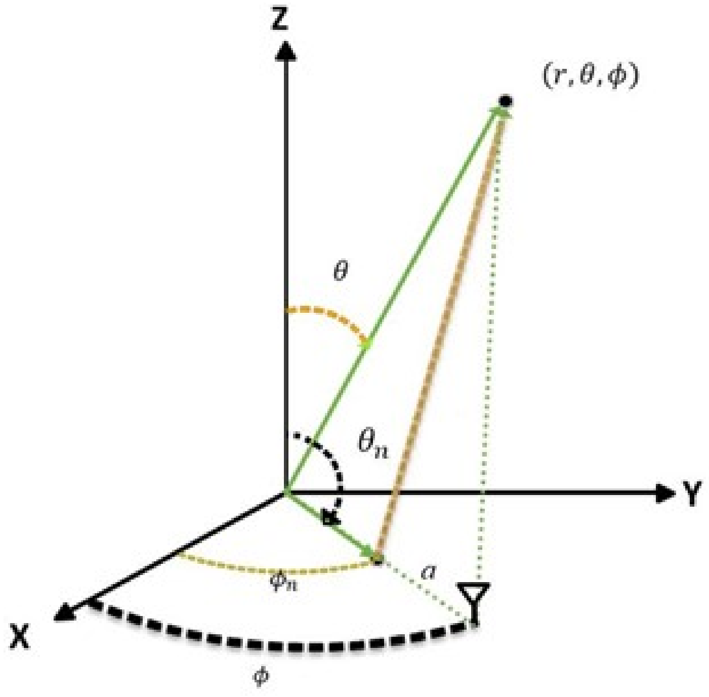
Figure 3.
SADDE flow chart.
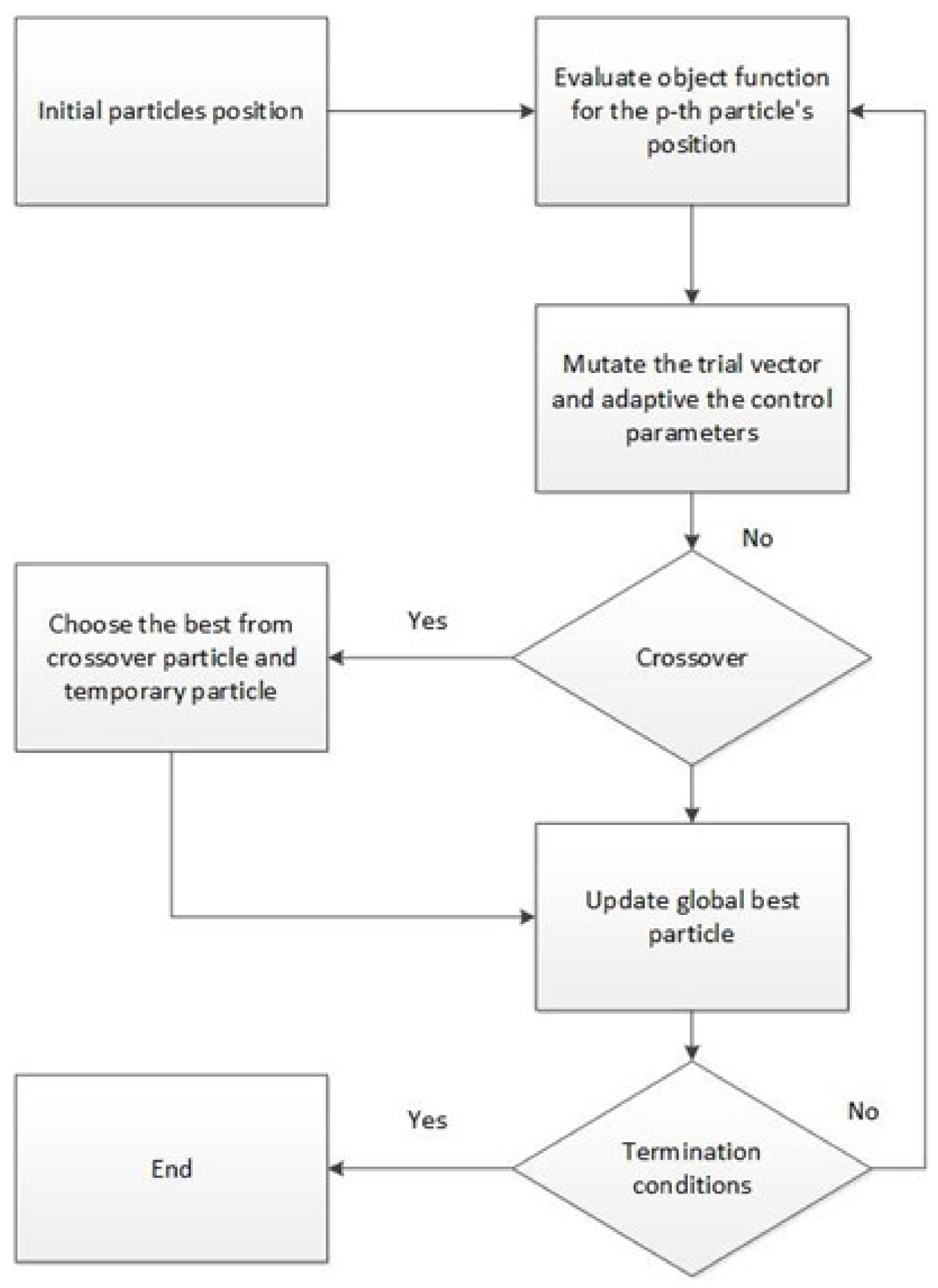
Figure 4.
Indoor environment layout.
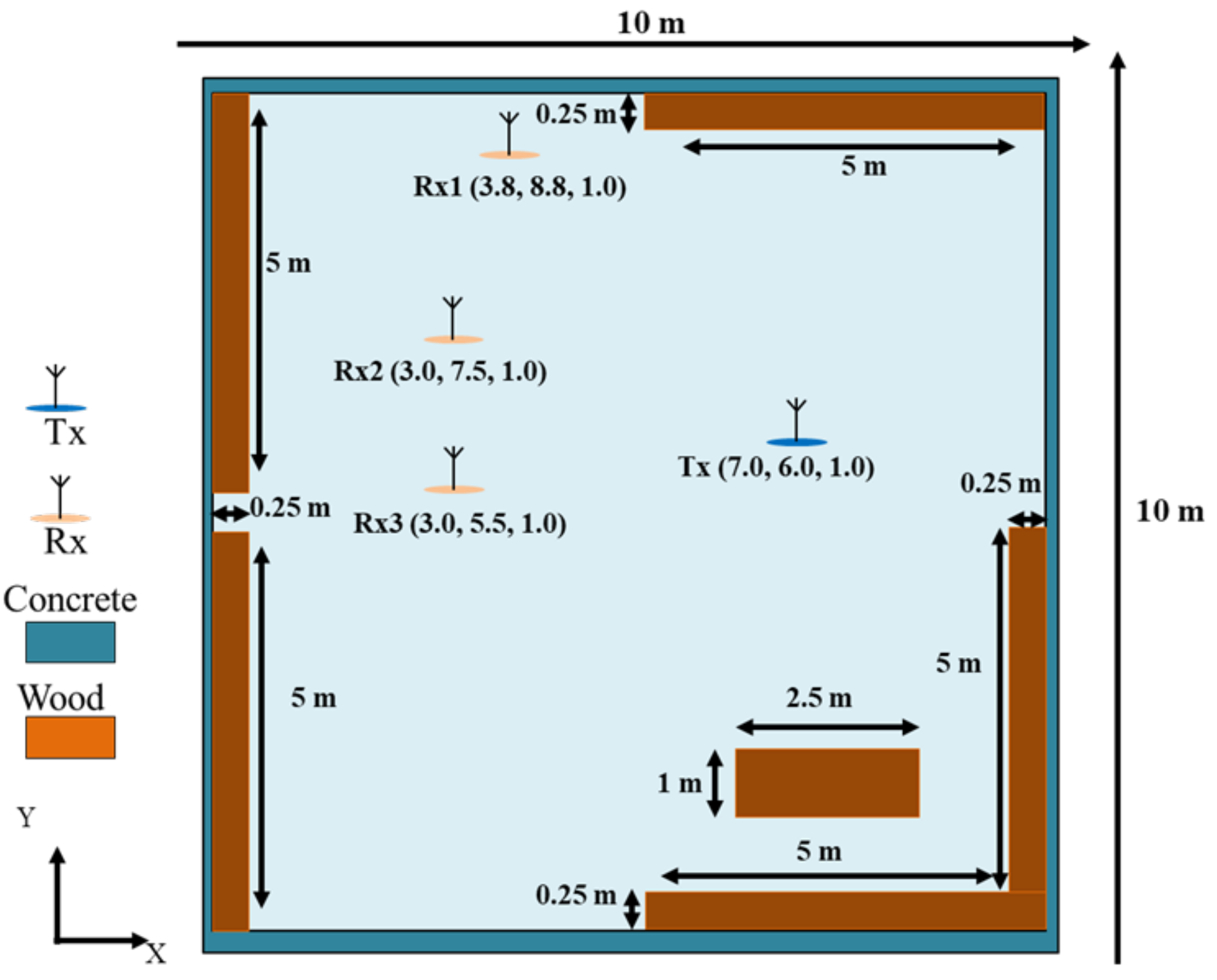
Figure 5.
Three different antenna array deployments: (a) circular; (b) triangular; and (c) rectangular.
Figure 5.
Three different antenna array deployments: (a) circular; (b) triangular; and (c) rectangular.
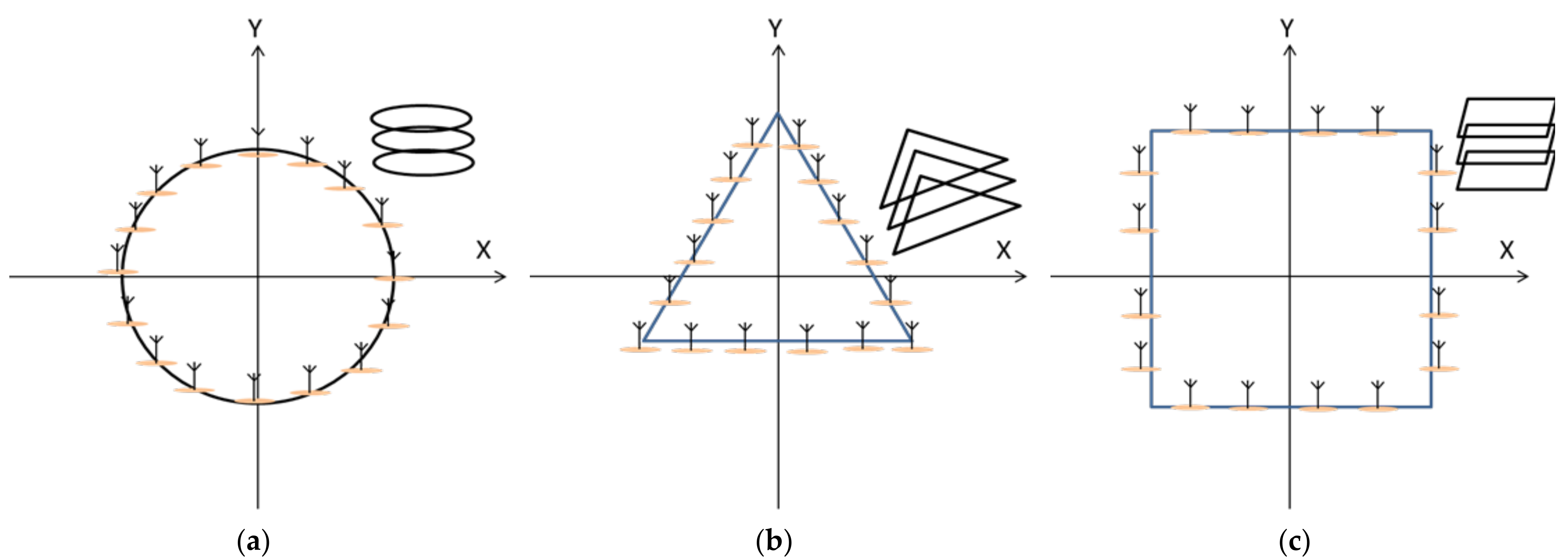
Figure 6.
Harvesting power ratios with different deployments with high resolution.

Figure 7.
Harvesting power ratios for different deployments with low resolution.
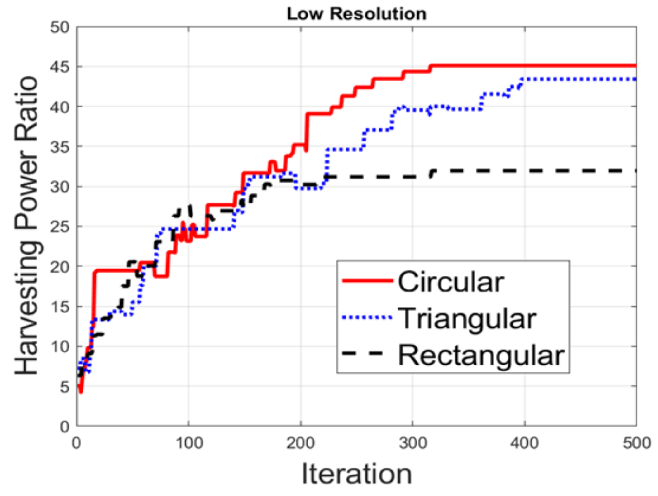
Figure 8.
BER for different deployments with high resolution.
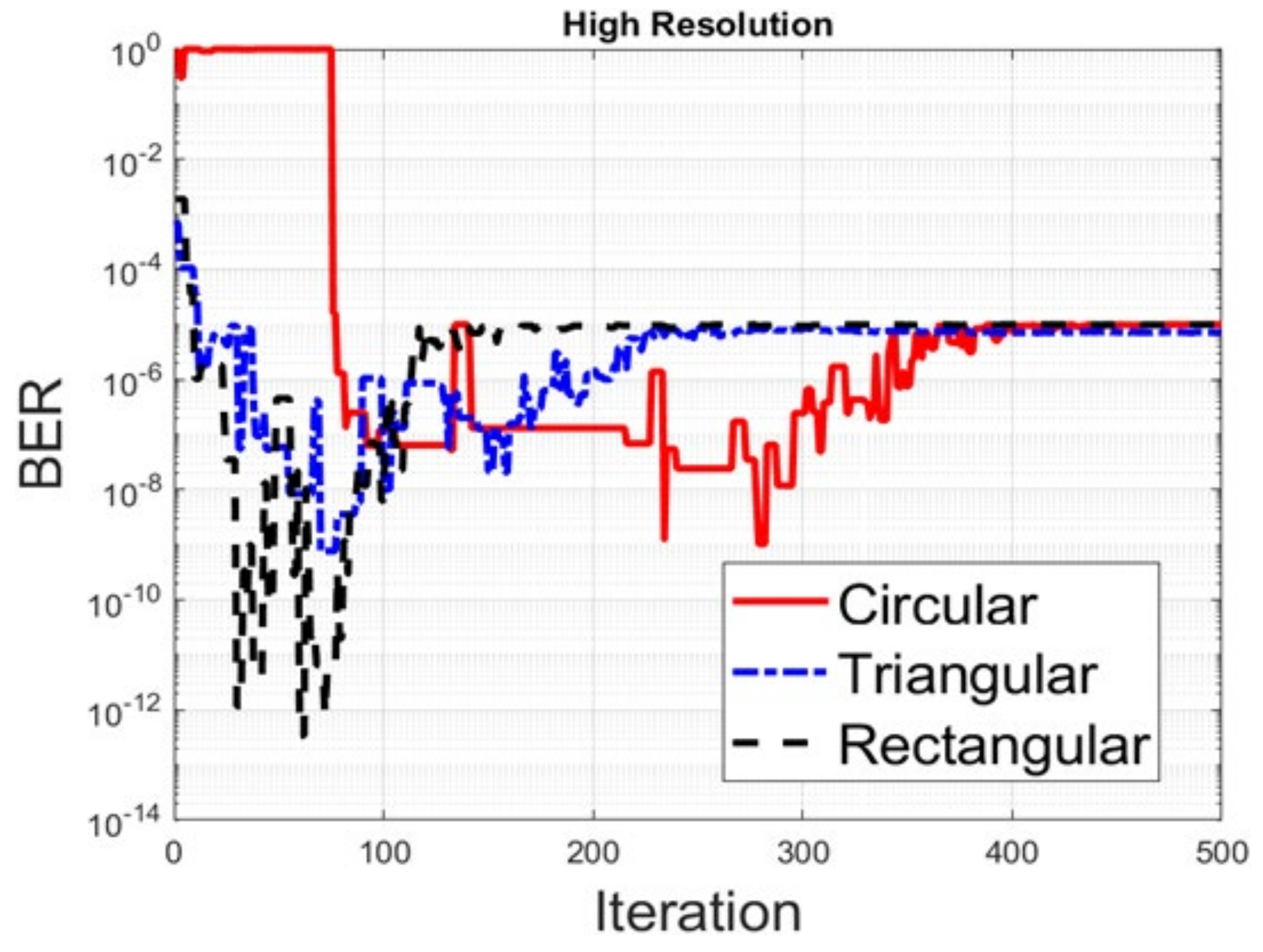
Figure 9.
BER for different deployments with low resolution.
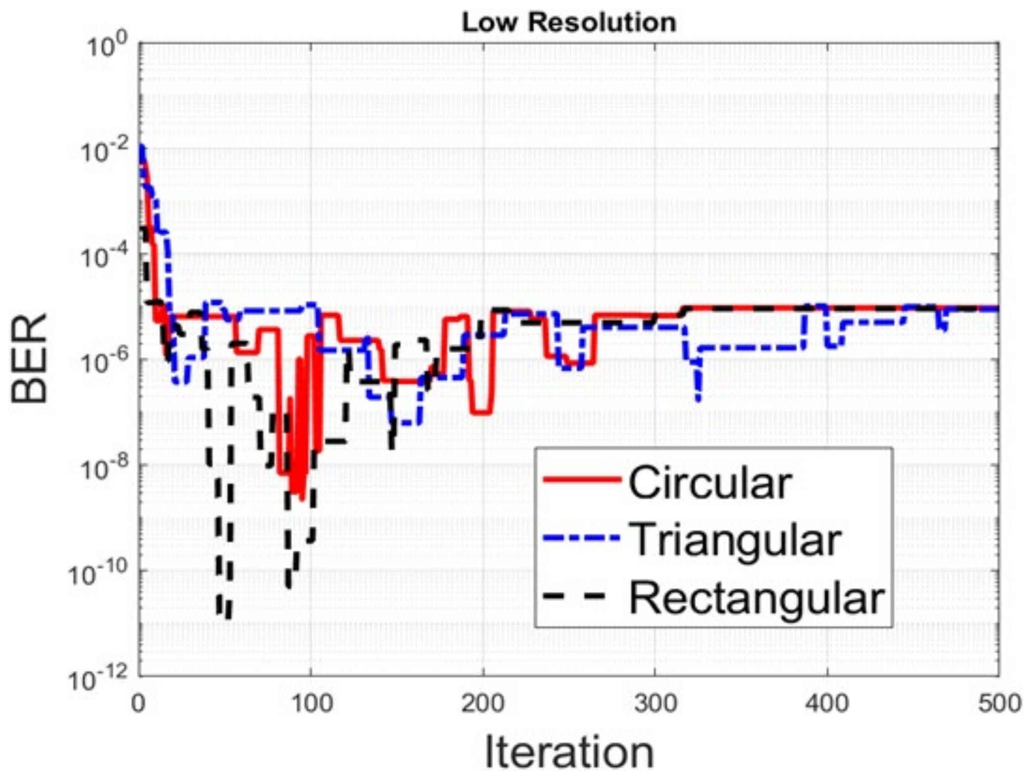
Figure 10.
Radiation pattern for the circular array: (a) high resolution; and (b) low resolution.

Figure 11.
Radiation pattern for the triangular array: (a) high resolution; and (b) low resolution.

Figure 12.
The optimization of pattern for the rectangular array: (a) high resolution; and (b) low resolution.
Figure 12.
The optimization of pattern for the rectangular array: (a) high resolution; and (b) low resolution.

Figure 13.
Harvesting power ratios for the high-resolution circular array.

Figure 14.
Harvesting power ratios for the high-resolution triangular array.

Figure 15.
Harvesting power ratios for the high-resolution rectangular array.

Figure 16.
Harvesting power ratios for the low-resolution circular array.
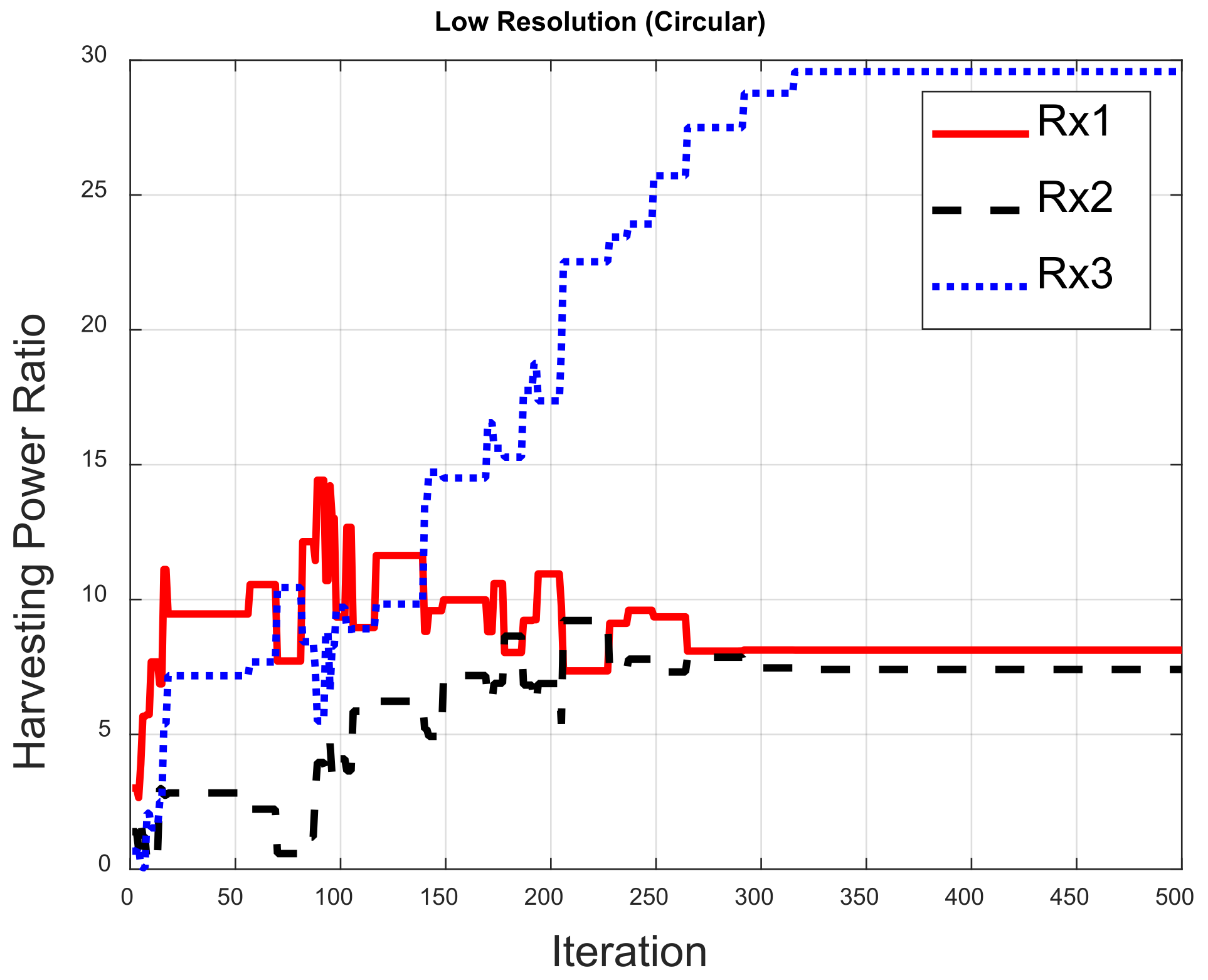
Figure 17.
Harvesting power ratios for the low-resolution triangular array.
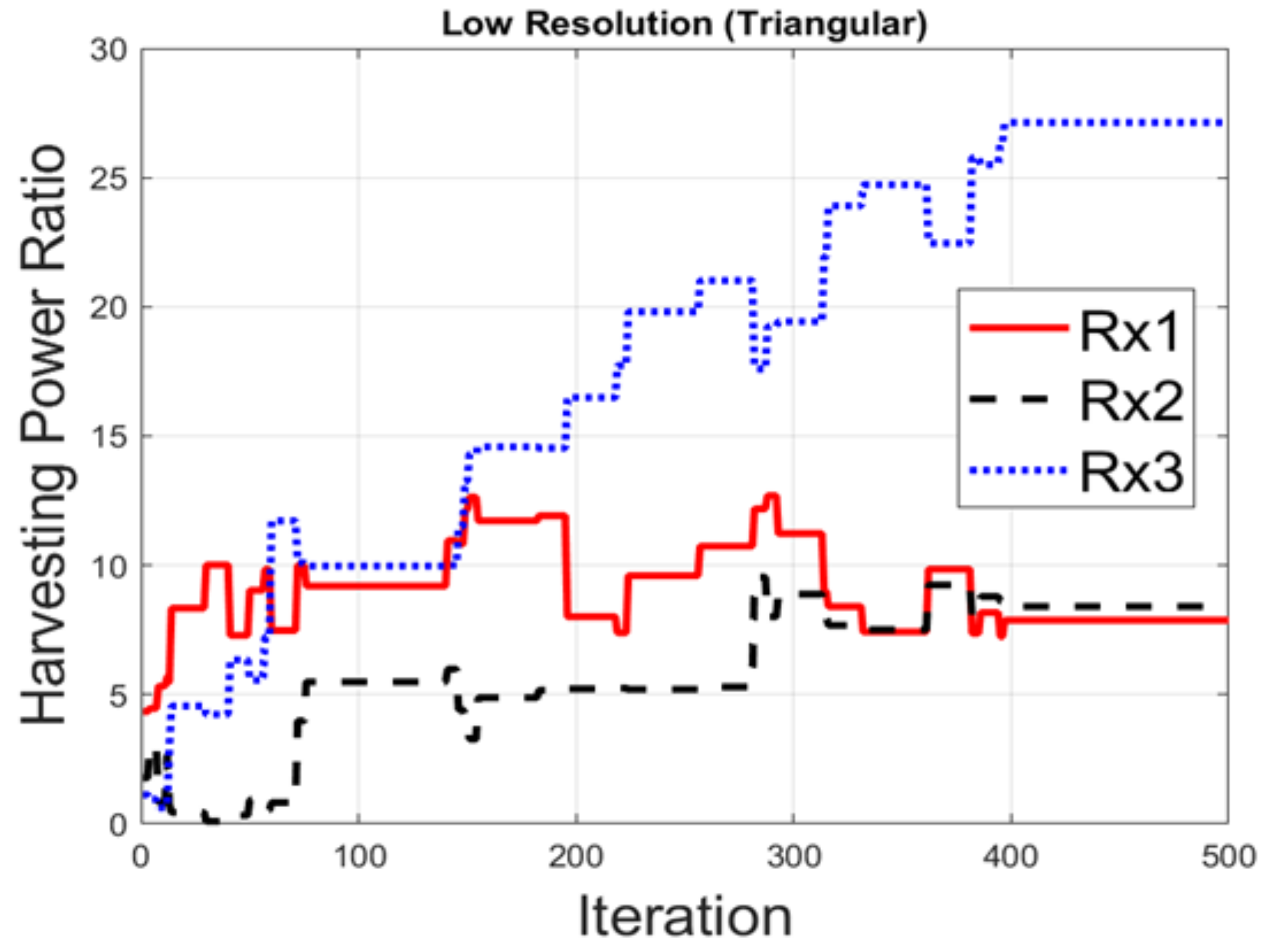
Figure 18.
Harvesting power ratios for the low-resolution rectangular array.
Publisher’s Note: MDPI stays neutral with regard to jurisdictional claims in published maps and institutional affiliations. |
© 2021 by the authors. Licensee MDPI, Basel, Switzerland. This article is an open access article distributed under the terms and conditions of the Creative Commons Attribution (CC BY) license (https://creativecommons.org/licenses/by/4.0/).
Share and Cite
MDPI and ACS Style
Chiu, C.-C.; Wu, H.-Y.; Chien, W.; Cheng, Y.-T.; Lim, E.H. Optimization of Different Deployments and Resolution of Antenna Arrays in SWIPT. Electronics 2022, 11, 19. https://doi.org/10.3390/electronics11010019
AMA Style
Chiu C-C, Wu H-Y, Chien W, Cheng Y-T, Lim EH. Optimization of Different Deployments and Resolution of Antenna Arrays in SWIPT. Electronics. 2022; 11(1):19. https://doi.org/10.3390/electronics11010019
Chicago/Turabian StyleChiu, Chien-Ching, Hung-Yu Wu, Wei Chien, Yu-Ting Cheng, and Eng Hock Lim. 2022. "Optimization of Different Deployments and Resolution of Antenna Arrays in SWIPT" Electronics 11, no. 1: 19. https://doi.org/10.3390/electronics11010019
Note that from the first issue of 2016, this journal uses article numbers instead of page numbers. See further details here.