
Comprehensive Overview of Backpropagation Algorithm for Digital Image Denoising


1
Department of Basic Science, College of Science and Theoretical Study, Saudi Electronic University, Dammam-Female Branch, Dammam 32242, Saudi Arabia
2
Department of Computer Applications, University Institute of Computing, Chandigarh University, Mohali 140413, India
3
School of Mathematics, University of Edinburgh, Edinburgh EH9 3FD, UK
4
Department of Mathematics, Faculty of Science, Jazan University, Jazan 45142, Saudi Arabia
*
Authors to whom correspondence should be addressed.
†
These authors contributed equally to this work.
Electronics 2022, 11(10), 1590; https://doi.org/10.3390/electronics11101590
Submission received: 18 April 2022
/
Revised: 7 May 2022
/
Accepted: 9 May 2022
/
Published: 17 May 2022
(This article belongs to the Topic Applied System on Biomedical Engineering, Healthcare and Sustainability)
Abstract
:Artificial ANNs (ANNs) are relatively new computational tools used in the development of intelligent systems, some of which are inspired by biological ANNs, and have found widespread application in the solving of a variety of complex real-world problems. It boasts enticing features as well as remarkable data processing capabilities. In this paper, a comprehensive overview of the backpropagation algorithm for digital image denoising was discussed. Then, we presented a probabilistic analysis of how different algorithms address this challenge, arguing that small ANNs can denoise small-scale texture patterns almost as effectively as their larger equivalents. The results also show that self-similarity and ANNs are complementary paradigms for patch denoising, as demonstrated by an algorithm that effectively complements BM3D with small ANNs, surpassing BM3D at a low cost. Here, one of the most significant advantages of this learning technique is that, once taught, digital images may be recovered without prior knowledge of the degradation model (noise/blurring) that caused the digital image to become distorted.
1. Introduction
Digital image denoising is an engineering and science area that investigates strategies for recovering an original scene from degraded data [1,2]. This field has long been studied in the signal processing, astronomy, and optics communities. Many of the techniques utilised in this domain have their roots in well-developed mathematical topics such as estimate theory, ill-posed inverse problem solution, linear algebra, and numerical analysis. Modeling the degradations, which are mainly blur and noise, and applying an inverse approach to produce an approximation of the original scene are the techniques utilised for image denoising.
However, in most real-world scenarios, significant a priori information regarding the blurring system’s degradation is rarely accessible. As a result, utilising limited information about the imaging system, we must estimate both the genuine picture and the blur from the degraded image attributes. In this study, we looked at picture noising [3,4,5], which is a specific sort of image degradation.
During acquisition, transmission, or recovery from the storage medium, images are frequently contaminated by noise. When an image is produced with a digital camera under low lighting settings or under other limitations/conditions, many dots can appear in the image (see Figure 1). The appearance of these dots (random behaviors of noisy signals) is caused by noise corrupting the real signals (unwanted signals). Images, movies, and other forms of signals are all corrupted by these disturbances.
The goal of the supervised learning algorithm [6,7,8] for digital image denoising is to eliminate noise such as this. Because a noisy image is unpleasant to look at, digital image denoising is required. As a result, some fine visual details may be misinterpreted for noise or vice versa. Different sorts of sounds impact digital photos [9,10,11].
Digital image denoising [12] is commonly thought of as a function that maps a noisy (corrupted) image to a cleaner version of that image. However, because the mapping from images to images is difficult, we chopped the image into possibly overlapping patches and learned mapping from a noisy patch to a clean patch in practice. All patches of noisy images were denoised independently using that map for image denoising of a particular noisy image, and then restored image patches were joined in such a way that we obtained an original image in denoised form (cleaner version restored image).
One thing to keep in mind is that the size of the picture patches has an impact on the denoising function’s quality. Many clean patches could explain a given noisy patch if the size of the image patches is small and the noise level is large. Here, we witnessed a necessary trade-off: very small patches lead to an easily modelled function but poor picture denoising results, whereas very big patches may lead to a better image denoising result but a difficult to model function [13,14,15,16,17].
Noise is not injective and thus not invertible when applied on a clean patch. As a result, finding a perfect denoising function is difficult. This problem can be solved by lowering the noise level and increasing the size of the image patches. A given noise could be explained by the presence of fewer clean patches. Large patches can thus achieve superior denoising outcomes than tiny ones, at least in theory [18,19,20].
We showed in this research that a simple MLP with supervised learning that maps noisy patches onto noise-free ones could reach state-of-the-art digital image denoising performance. In order to make this possible, the following components were integrated [21,22]:
- The MLP’s capacity was chosen to be large enough to accommodate a suitable number of hidden layers and hidden layer neurons;
- The image patch size was selected to ensure that a noisy image patch has sufficient information to recover a noise-free version of the original input image;
- The chosen training set was large enough to allow for on-the-fly generation of training samples by corrupting noise-free patches with noise.
2. Artificial ANNs
An ANN, parallel distributed processing systems (PDPs) and connectionist systems, is a “black box” technique for predictive modeling that requires all characters defining the unknown circumstance to be provided to a trained ANN for identification (prediction) [19]. Advantages and disadvantages of ANNs are listed in Table 1. An ANN is designed to imitate the central nervous system’s organisational principles, with the goal that the ANN’s biologically inspired computing skills make performing cognitive and sensory tasks easier and more satisfying than with conventional serial processors. Information processing is a system that has a large number of highly interconnected processing neurons and is biologically inspired computing capacity of ANN systems such as human brains. In PDPs, these neurons collaborate to learn from the input data, coordinate internal processing, and maximise the final output. The artificial neural network (ANN) is a mathematical model of the human neural architecture that reflects its “learning” and “generalization” capacities. Artificial ANNs (ANNs) are a type of AI [1]. An artificial neural network (ANN) is a classification system that can be implemented in either hardware or software. During the training phase, it is an adaptive system that modifies its structure or the internal information that travels through the network. Because of qualities including strong non-linear mapping capacity, high learning accuracy, and good robustness, ANN is widely employed in various fields [23]. A feedforward ANNs model called a multi-layer perceptron (MLP) maps sets of input data to a set of relevant outputs. An MLP is a directed graph made up of multiple layers of nodes, each fully connected to the next. Each node is a neuron (or processing element) with a non-linear activation function, with the exception of the input nodes. Backpropagation is a supervised learning approach used by MLP to train the network. The MLP is a modified linear perceptron that can discriminate data that are not linearly separable [24,25,26].
3. Problem Specific Approach for ANNs Development
The various phases in the problem-specific approach for ANN development constitute a cycle of six phases [29,30], shown in Figure 2:
- Phase 1 (problem description and formulation): This phase is primarily reliant on a thorough grasp of the problem, especially the “cause-effect” relationships. Before deciding on a modelling technique, the advantages of ANNs over alternative techniques (if available) should be weighed;
- Phase 2 (System Design): This is the initial phase in the actual ANN design, in which the modeller selects the appropriate type of ANN and learning algorithm for the task. Data collecting, data preprocessing to fit the type of ANN utilised, statistical data analysis, and data splitting into three unique subsets are all part of this phase (training, test, and validation subsets);
- Phase 3 (System Realisation): This phase entails training the network with the training and test subsets while also analysing the prediction error to gauge network performance. The design and performance of the final network can be influenced by the optimal selection of numerous parameters (e.g., network size, learning rate, number of training cycles, tolerable error, etc.). If practicable, breaking the problem down into smaller sub-problems and building an ensemble of networks could improve overall system accuracy. The modeller is now back in phase 2;
- Phase 4 (System Verification): Although network construction includes ANN testing against test data while training is in progress, it is best to practise (if data permits) using the validation subset to assess the best network for its generalisation capabilities. The goal of verification is to ensure that the ANN-based model can appropriately respond to cases that have never been utilised in network construction. Comparing the performance of the ANN-based model to that of other methodologies (if available) such as statistical regression and expert systems is also part of this phase.
- Phase 5 (System Implementation): This phase entails integrating the network into a suitable operating system, such as a hardware controller or computer software. Before releasing the integrated system to the end user, it should be thoroughly tested.
- Phase 6 (System Maintenance): This phase entails upgrading the produced system as the environment or system variables change (e.g., new data), which necessitates a new development cycle.
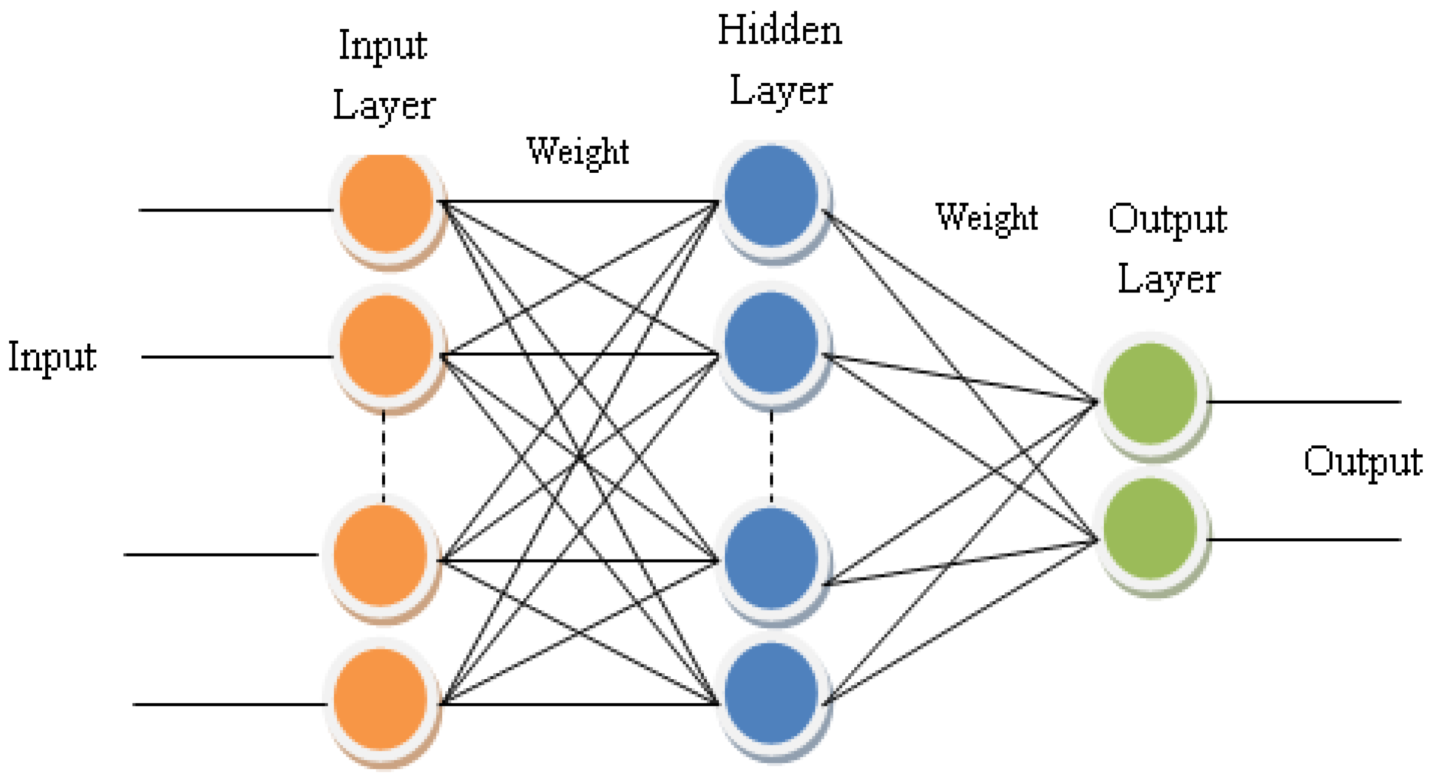
4. Multi-Layer Perceptron ANNs
A Multi-Layer Perceptron (MLP) is an artificial neural network (ANN) made up of simple neurons called perceptrons. It is a feedforward artificial neural network (ANN) that maps sets of input data to a set of relevant outputs. The MLP is a deep ANN since it has three or more layers of non-linearly active neurons (an input, an output, and one or more hidden layers), as shown in Figure 3. Weight is a type of data that the neural network uses to solve a problem. Weights can be set to zero or calculated using a variety of methods. The normalised initialisation is used:
where and are the number of neurons in the input side and output side of the layer, respectively.
In a neural network, weight initialisation is a critical criterion. The weight changes represent the neural network’s overall performance. If these values are 0 (since there is no direct link between input and output), the gradients calculated during the trial will also be 0, and the network will not learn. In order to discover the ideal value for the cost function, further learning attempts with varying initial weights are suggested (minimum error).
MLP is made up of numerous layers of neurons in a feedforward network (directed graph), with each layer fully connected to the one before it, each with a non-linear activation function. If MLP has a linear activation function in all neurons, which is a linear function that maps the weighted inputs to each neuron’s output, then any number of layers can be lowered from the usual two-layer input-output ANNs [31].
The input layer neurons merely act as buffers, spreading the input signals out (i = 1, 2, …, n) to the hidden layer neurons. Each hidden layer neuron j (j = 1, 2, …, m), see Figure 3, sums its input signals after weighing them with the strength of the respective input-hidden layer connections (weights of the input-hidden layer) and (weights of hidden and output layer) from the input layer is the bias (: bias of hidden layer and : bias of output layer), and computes its output.
is the sum of the activation functions (hidden layer activation function) and (output layer activation function).
Here, Figure 4 shows the basic architecture of MLP ANN.
5. Supervise Learning Algorithm
We fed input data and correct data to the network in the supervised learning method. The input data are propagated in a forward manner through the network until it reaches the output neurons, where it is compared to the correct data, and the error is calculated. We do not need to change anything in the network if the output contains no or minimal errors. If there is an error, we must modify the weights in the network to ensure that the network delivers accurate output in future learning, as shown in Figure 5. Supervised learning is the term for this method of weight modification. The backpropagation training technique, often known as the generalised delta rule, is one of the most commonly used supervised learning algorithms in real-world applications.
MLP-ANNs are trained using the backpropagation (error backpropagation) algorithm. The rules of supervised learning (error corrective learning) are used in this method [32,33,34]. This algorithm involves two passes through the MLP-distinct ANN’s layers: forward and reverse training. A pattern activity is applied to the MLP-input ANN’s neurons in forward training, and its influence propagates across the network layer by layer, producing a set of output as the network’s real-time response. The network’s weights (synaptic weights) are fixed in this situation. All weights are modified according to the supervised learning rule during backward training.
In order to generate an error signal, the network’s real-time response is deducted from the desired response. This error signal is then passed on to the rest of the network. Adjusted all the weights to bring the network’s real-time response statistically closer to the target response. In order to reduce the inaccuracy, all of the weights are changed using the generalised Delta rule [35,36].
The two most commonly used neuron activation functions for the neurons in Figure 3 are Sigmoidal (it is similar to the step function) and Tansig activation functions, . Both functions are continuously differentiable everywhere and typically have the following mathematical forms:
Supervised Learning Algorithm notations used are:
- Input to neuron j of layer l;
- Weight from layer (l−1) neuron i (means weights of previous layer neuron i) to layer l neuron j;
- Sigmoidal transfer function;
- Bias of neuron j of layer l;
- Output of neuron j in layer l;
- Target value of neuron j of the output layer.
5.1. The Error Calculation
Given a set of training data points tj and output layer Oj, we can write the error as:
We let the error of the MLP-ANN for a single training iteration be denoted by E. We want to calculate , the rate of change of the error with respect to the given connective weight, so we can minimise it, see Figure 6. Now consider two cases: the neuron is an output neuron, or it is in a hidden layer.
5.2. Output Layer Neurons
As, is a constant.
is where is input and output of neuron j.
Therefore, the output of the neuron j with a product of weight is . For notation purposes, is defined to be the expression , so we can rewrite the above equation as:
, where .
5.3. Hidden Layer Neurons
As, () is the input of neuron k to the output of neuron j.
, where = .
Therefore, run the MLP-ANN forward training with input data to obtain the desired response. For each output neuron, compute . For each hidden-layer neuron, calculate . Update the weights and biases as follows:
Therefore, apply and , where learning rate, usually less than 1.
5.4. ANN Parameter
When designing a neural network, a lot of distinct parameters must be determined:
5.4.1. Number of Hidden Layer Neurons
Data type: Integer_Domain [1, ∞]
Typical value: 8
5.4.2. Learning Rate ()
Learning rate is a training parameter that regulates the weight and bias adjustments in the training algorithm’s learning. The greater the value of , the greater the step and the faster the convergence. The learning algorithm takes a long time to converge if the value of is small.
Data type: Real_Domain [0, 1]
Typical value: 0.3
5.4.3. Momentum
Momentum is simply a fraction µ of the prior weight update added to the recent one. The momentum parameter is employed to keep the system from settling into a local minimum, often known as a saddle point. A high momentum parameter can also aid in speeding up the system’s convergence. Setting the momentum parameter too high, on the other hand, runs the danger of overshooting the minimum, causing the system to become unstable. A low momentum coefficient does not dependably avoid local minima and also slows down the system’s training.
Data type: Real_Domain [0, 1]
Typical value: 0.5
5.4.4. Training Type
0 = Train by Epoch
1 = Train by minimum error
Data type: Integer Domain: [0, 1]
Typical value: 1
5.4.5. Epoch
When the number of iterations reaches epoch, the training comes to an end. This is the maximum number of iterations when training by minimum error.
Data type: Integer_Domain [1, ∞]
Typical value: 5000
5.4.6. Minimum Error (Only for Training by Minimum Error)
Data type: Real_Domain [0, 0.5]
Typical value: 0.01
5.5. Delta Learning Rule
The delta learning rule is a learning rule for updating the weights of the inputs to artificial neurons in ANNs. It is a special case of the backpropagation learning algorithm. In this rule, the input weights are continuously updated by taking the difference (the delta) between the desired response and the real-time response. This rule updates the weights in such a way that the mean square error of the designed ANN should be minimised. It is significant to confirm that the input data set is well randomised. A well-ordered and structured data set (in this case, designed ANN is incapable of learning the problem) cannot converge the desired response.
5.6. Gradient Descent (GD) Learning Rule
This learning strategy (similar to the delta rule) updates the network weights and biases in the direction of the most rapidly decreasing performance function, i.e., the negative of the gradient. It is very beneficial for functions with a lot of dimensions. The new weight vector is recalculated based on:
The minus sign denotes that the new weight vector is travelling in the opposite direction as the gradient.
5.7. Gradient Descent Backpropagation with Momentum (GDM)
Momentum allows an ANN to adapt to the latest trends in the error surface as well as the local gradient. The ANN can disregard minor characteristics in the error surface because of momentum. An ANN without momentum may become stuck in a low local minimum. An ANN can slip through such a low momentum. By making weight modifications equal to the fraction sum of the previous weight change and the new change indicated by the gradient descent backpropagation rule, momentum can be added to the backpropagation method learning. A momentum constant µ mediates the magnitude of the influence that the last weight shift is allowed to have. When µ is set to 0, a weight change is purely determined by the gradient. When µ is 1, the new weight modification is equal to the previous weight modification, and the gradient is ignored. The new weight vector is modified as follows [37,38]:
Variable learning rate gradient descent backpropagation uses a bigger learning rate when the intended ANN model is far from the desired response and a smaller learning rate when the planned ANN model is near the desired response to speed up the convergence time. As a result, the new weight vector is updated using the variable learning rate as follows:
where and .
ANNs learning iterations, which are referred to be epochs, consist of two phases [39]:
- For each training pattern in ANNs, feedforward propagation simply calculates the output values;
- Backward propagation is where an erroneous signal is sent backward from the output layer to the input layer. The backpropagated error signal is used to alter the weights.
6. Results
Self-similarity is a fundamental property of nature, but its application in image processing is limited due to the finite resolution of digital images and the presence of noise. We have used five test images, see Figure 7. As a result, see Table 2, a self-similarity-guided denoising algorithm must adapt the patch size to the scale of the image content as well as the noise level. Similar neighbors may not exist if a patch is too large in relation to its surroundings. If a patch is too small in comparison to the noise level, however, it is difficult to appropriately identify similar patches among its nearby candidates using block-matching. It is thus difficult to restore tiny scale texture patterns when there is a lot of noise.
ANNs are a feasible answer since they are specifically trained to approximate a conditional expectation, which makes them scale and noise conscious. However, they require an even broader observation window to appropriately handle large-scale and often highly organised patterns on their own, which unfortunately comes at a considerable computational cost due to their extensive hidden layers and deep architectures.
To scale down big ANNs, one must make use of self-similarity and ANNs’ complementary nature. Therefore, by using a self-similarity-based method for larger-scale patterns and small neural nets for smaller-scale patterns, one can have the best of both worlds without having to worry about the technical details of patch size. Despite this, a filter based on a hard scale classification is more prone to errors than the ideal conditional expectation decomposition’s soft weighting scheme, and the accuracy of the [11] texture detector has not been affected by noise.
7. Importance of ANN in Various Fields
ANNs have a number of advantages that make them ideal for a variety of issues and situations [40]:
- ANNs can learn and model non-linear and complicated interactions, which is critical because many of the relationships between inputs and outputs in real life are non-linear and complex;
- ANNs can generalise—after learning from the original inputs and their associations, the model may infer unknown relationships from unknown data, allowing it to generalise and predict on unknown data;
- ANN does not impose any limits on the input variables, unlike many other prediction algorithms (such as how they should be distributed). Furthermore, several studies demonstrated that ANNs could better predict heteroskedasticity, or data with high volatility and non-constant variance, because of their capacity to learn latent links in the data without imposing any predefined relationships.
ANNs are important because of some of their great properties:
- Image Processing and Character Recognition: ANNs play an important role in image and character recognition because of their ability to take in a large number of inputs, process them, and infer hidden as well as complex, non-linear correlations. Character recognition, such as handwriting recognition, has a wide range of applications in fraud detection and even national security assessments. Image recognition is a rapidly evolving field with numerous applications ranging from social media facial recognition to cancer detection in medicine to satellite data processing for agricultural and defense uses. Deep ANNs [6,7], which form the backbone of “deep learning”, have now opened up all of the new and revolutionary developments in computer vision, speech recognition, and natural language processing—prominent examples being self-driving cars, thanks to ANN research [16,17,20,40];
- Forecasting: Forecasting is widely used in everyday company decisions (such as sales, the financial allocation between products, and capacity utilisation), economic and monetary policy, and finance and the stock market. Forecasting difficulties are frequently complex; for example, predicting stock prices is a complicated problem with many underlying variables (some known, some unseen). Traditional forecasting models have flaws when it comes to accounting for these complicated, non-linear relationships. Given its capacity to model and extract previously overlooked characteristics and associations, ANNs can provide a reliable alternative when used correctly. ANN also has no restrictions on the input and residual distributions, unlike classical models. For example, recent breakthroughs in the use of LSTM and Recurrent ANNs for forecasting are driving more research on the subject [4,5,6,11,40].
8. Conclusions and Future Work
We focused on the conditional expectation in this paper because it is not only essential for understanding most patch-based denoising techniques, but it is also naturally easier to evaluate and approximate than the underlying law. Furthermore, we demonstrated through studies that small ANNs have two advantages: they can survive considerably higher noise on small-scale texture patterns than BM3D and its derivatives, and the notion of scale is clear due to their set input size. Moreover, the backpropagation learning algorithm is an efficient technique for denoising of digital images without prior knowledge of the degradation model (noise/blurring). This algorithm works perfectly once an ANN is trained properly. Here, we see more training data samples give good performance for the existing model. Since the ANN model used here is complicated if the number of hidden layers goes above the typical value, which degrades the performance of the network. One of the expected domains to work in the future is the use of multiple copy multi-layer perceptron (MC-MLP), patch selection, self-constructing ANN model, etc., to obtain better results.
Author Contributions
Conceptualisation, S.K. and A.S.; methodology, S.K.; software, S.K.; validation, S.K. and A.S.; formal analysis, S.K., M.S. and A.S.; investigation, resources, and data curation, S.K., M.A. and A.S.; writing—original draft preparation, S.K. and A.S.; writing—review and editing, S.K., M.S. and M.A.; supervision, A.S.; project administration, S.K.; funding acquisition, M.A. All authors have read and agreed to the published version of the manuscript.
Funding
This research received no external funding.
Institutional Review Board Statement
Not applicable.
Informed Consent Statement
Not applicable.
Data Availability Statement
Not applicable.
Conflicts of Interest
The authors declare no conflict of interest.
References
- Banhom, M.R.; Katsaggelos, A.K. Digital Image Denoising. IEEE Signal Process. Mag. 1997, 14, 24–41. [Google Scholar] [CrossRef]
- Yang, Y.; Zhang, T.; Hu, J.; Xu, D.; Xie, G. End-to-End Background Subtraction via a Multi-Scale Spatio-Temporal Model. IEEE Access 2019, 7, 97949–97958. [Google Scholar] [CrossRef]
- Jain, A.K. Fundamentals of Digital Image Processing. In Control of Color Imaging Systems; CRC Press: Boca Raton, FL, USA, 2018. [Google Scholar] [CrossRef]
- Thakur, R.S.; Yadav, R.N.; Gupta, L. State-of-art analysis of image denoising methods using convolutional neural networks. IET Image Process. 2019, 13, 2367–2380. [Google Scholar] [CrossRef]
- Bouwmans, T.; Javed, S.; Sultana, M.; Jung, S.K. Deep neural network concepts for background subtraction:A systematic review and comparative evaluation. Neural Netw. 2019, 117, 8–66. [Google Scholar] [CrossRef] [Green Version]
- Zhang, T.; Zhang, X.; Ke, X.; Liu, C.; Xu, X.; Zhan, X.; Wang, C.; Ahmad, I.; Zhou, Y.; Pan, D.; et al. HOG-ShipCLSNet: A Novel Deep Learning Network with HOG Feature Fusion for SAR Ship Classification. IEEE Trans. Geosci. Remote Sens. 2022, 60, 5210322. [Google Scholar] [CrossRef]
- Zhang, T.; Zhang, X. ShipDeNet-20: An Only 20 Convolution Layers and <1-MB Lightweight SAR Ship Detector. IEEE Geosci. Remote Sens. Lett. 2021, 18, 1234–1238. [Google Scholar] [CrossRef]
- Zhang, T.; Zhang, X. Squeeze-and-Excitation Laplacian Pyramid Network with Dual-Polarization Feature Fusion for Ship Classification in SAR Images. IEEE Geosci. Remote Sens. Lett. 2022, 19, 4019905. [Google Scholar] [CrossRef]
- Kushwaha, S.; Singh, R.K. Study of Various Image Noises and Their Behavior. Int. J. Comput. Sci. Eng. 2015, 3, 2347–2693. [Google Scholar]
- Protter, M.; Elad, M. Image Sequence Denoising via Sparse and Redundant Representations. IEEE Trans. Image Process. 2010, 18, 842–861. [Google Scholar] [CrossRef]
- Zhao, C.; Basu, A. Dynamic Deep Pixel Distribution Learning for Background Subtraction. IEEE Trans. Circuits Syst. Video Technol. 2020, 30, 4192–4206. [Google Scholar] [CrossRef]
- Zhang, T.; Zhang, X.; Ke, X. Quad-FPN: A Novel Quad Feature Pyramid Network for SAR Ship Detection. Remote Sens. 2021, 13, 2771. [Google Scholar] [CrossRef]
- LeCun, Y.; Bottou, L.; Orr, G.; Muller, K. Efficient Backprop. In ANNs, Tricks of the Trade, Lecture Notes in Computer Science LNCS 1524; Springer: Berlin/Heidelberg, Germany, 1998; Available online: http://leon.bottou.org/papers/lecun-98x (accessed on 5 April 2022).
- Elad, M.; Aharon, M. Image Denoising Via Sparse and Redundant Representations over Learned Dictionaries. IEEE Trans. Image Process. 2006, 15, 3736–3745. [Google Scholar] [CrossRef] [PubMed]
- Kushwaha, S.; Rai, A. IoT with AI: Requirements and Challenges. Gorteria 2022, 35, 105–114. [Google Scholar]
- Kushwaha, S.; Singh, R.K. Optimization of the proposed hybrid denoising technique to overcome over-filtering issue. Biomed. Eng. Biomed. Tech. 2019, 64, 601–618. [Google Scholar] [CrossRef] [PubMed]
- Kushwaha, S.; Singh, R.K. Robust denoising technique for ultrasound images by splicing of low rank filter and principal component analysis. Biomed. Res. 2018, 29, 3444–3455. [Google Scholar] [CrossRef] [Green Version]
- Burger, H.C.; Schuler, C.J.; Harmeling, S. Image denoising with multi-layer perceptrons, part 1: Comparison with existing algorithms and with bounds. arXiv 2012, arXiv:1211.1544. [Google Scholar]
- Luisier, F.; Blu, T.; Unser, M. Image denoising in mixed poisson—gaussian noise. IEEE Trans. Image Process. (TIP) 2011, 20, 696–708. [Google Scholar] [CrossRef] [Green Version]
- Kushwaha, S. An Efficient Filtering Approach for Speckle Reduction in Ultrasound Images. Biomed. Pharmacol. J. 2017, 10, 1355–1367. [Google Scholar] [CrossRef]
- Levin, A.; Nadler, B. Natural Image Denoising: Optimality and Inherent Bounds. In Proceedings of the IEEE Conference on Computer Vision and Pattern Recognition (CVPR), Washington, DC, USA, 20–25 June 2011; pp. 2833–2840. [Google Scholar]
- Kushwaha, S.; Singh, R.K. Performance Comparison of Different Despeckled Filters for Ultrasound Images. Biomed. Pharmacol. J. 2017, 10, 837–845. [Google Scholar] [CrossRef]
- Gnana Sheela, K.; Deepa, S.N. Review on methods to fix number of hidden neurons in ANNs. Math. Probl. Eng. 2013, 2013, 11. [Google Scholar]
- Rosenblatt, X.F. Principles of Neurodynamics: Perceptrons and the Theory of Brain Mechanism; Spartan Books: Washington, DC, USA, 1961. [Google Scholar]
- Kushwaha, S.; Singh, R.K. An Efficient Approach for Denoising Ultrasound Images using Anisotropic Diffusion and Teaching Learning Based Optimization. Biomed. Pharmacol. J. 2017, 10, 805–816. [Google Scholar] [CrossRef]
- Kushwaha, S. Mathematical Analysis of Robust Anisotropic Diffusion Filter for Ultrasound Images. Int. J. Comput. Sci. Eng. 2016, 4, 152–160. [Google Scholar]
- Zeng, A.K.D.; Zhu, M. Combining background subtraction algorithms with convolutional neural network. J. Electron. Imaging 2019, 28, 013011. [Google Scholar] [CrossRef]
- Zhao, C.; Hu, K.; Basu, A. Universal Background Subtraction Based on Arithmetic Distribution Neural Network. IEEE Trans. Image Process. 2022, 31, 2934–2949. [Google Scholar] [CrossRef] [PubMed]
- Basheer, I.A.; Hajmeer, M. Artificial ANNs: Fundamentals, computing, design, and application. ELSEVIER J. Microbiol. Methods 2000, 43, 3–31. [Google Scholar] [CrossRef]
- Asokan, A.; Anitha, J. Adaptive Cuckoo Search based optimal bilateral filtering for denoising of satellite images. ISA Trans. 2020, 100, 308–321. [Google Scholar] [CrossRef]
- Erhan, D.; Courville, A.; Bengio, Y. Understanding Representations Learned in Deep Architectures; Technical Report 1355; Université de Montréal/DIRO: Montreal, QC, Canada, 2010; pp. 1–25. [Google Scholar]
- Bengio, Y.; Glorot, X. Understanding the difficulty of training deep feedforward ANNs. In Proceedings of the Artificial Intelligence and Statistics Conference (AISTATS), Sardinia, Italy, 13–15 May 2010; Volume 9, pp. 249–256. [Google Scholar]
- Kushwaha, S.; Singh, R.K. Study and Analysis of Various Image Enhancement Method using MATLAB. Int. J. Comput. Sci. Eng. 2015, 3, 15–20. [Google Scholar]
- Lim, L.A.; Keles, H.Y. Learning multi-scale features for foreground segmentation. Pattern Anal. Appl. 2020, 23, 1369–1380. [Google Scholar] [CrossRef] [Green Version]
- Artificial ANNs/Competitive Models. Available online: www.wikibooks.org/wiki/Artificial_Neural_Networks/Competitive_Models (accessed on 5 April 2022).
- Chang, H.H.; Lin, Y.J.; Zhuang, A.H. An Automatic Parameter Decision System of Bilateral Filtering with GPU-Based Acceleration for Brain MR Images. J. Digit. Imaging 2019, 32, 148–161. [Google Scholar] [CrossRef]
- Dao, V.N.P.; Vemuri, V.R. A performance comparison of different back propagation ANNs methods in computer network intrusion detection. Differ. Equ. Dyn. Syst. 2002, 10, 201–214. [Google Scholar]
- Kumar, M.; Mishra, S.K. A Comprehensive Review on Nature Inspired Neural Network based Adaptive Filter for Eliminating Noise in Medical Images. Curr. Med. Imaging 2020, 16, 278–287. [Google Scholar] [CrossRef] [PubMed]
- Engelbrecht, A.P. Computational Intelligence: A Introduction, 2nd ed.; John Wiley and Sons Ltd.: Chichester, UK, 2007. [Google Scholar]
- Liu, S.; Chang, R.; Zuo, J.; Webber, R.J.; Xiong, F.; Dong, N. Application of Artificial ANNs in Construction Management: Current Status and Future Directions. Appl. Sci. 2021, 11, 9616. [Google Scholar] [CrossRef]
Figure 1.
Basic blocks of a digital camera and possible sources of noise.

Figure 2.
The various phases in problem-specific approach for ANN development.

Figure 3.
Details of multi-layer perceptron ANNs process.

Figure 4.
Basic structure of MLP ANN.

Figure 5.
Block diagram of supervised learning algorithms.

Figure 6.
Neural Network training and validation using BP algorithm.

Figure 7.
Test images: (a) Baboon; (b) F16; (c) House; (d) Lena; (e) Peppers. All images are of dimension 256 × 256.
Figure 7.
Test images: (a) Baboon; (b) F16; (c) House; (d) Lena; (e) Peppers. All images are of dimension 256 × 256.


| Advantages | Disadvantages |
|---|---|
| For specific requirements, the hidden layer structure can be put up in a variety of ways. | The model’s intricacy may result in over-fitting or under-fitting. |
| Multiple goal outputs can be set without increasing the challenge greatly. | There are no specific network design principles or recommendations. |
| There are a variety of challenges that can be classified as complex regression problems or classification tasks. | Low learning rate and local optimal. |
| Multivariable and non-linear issues. | Extrapolation beyond the data range performs poorly. |
| Problems arising from a lack of knowledge or experience. | Difficulty in expressing the decision’s rationale. |
| The link between factors is unclear. | Weight and other essential factors are difficult to determine. |
Table 2.
Algorithm comparison in PSNR [dB].
| Gaussian Noise Standard Deviation | Test Image Number | Performance Comparison of Different Filters for All Images | |||||
|---|---|---|---|---|---|---|---|
| [16] | [17] | [4] | [5] | [6] | [11] | ||
| σ = 10 | (a) | 35.12 | 35.67 | 35.48 | 36.82 | 36.51 | 36.11 |
| (b) | 40.14 | 44.56 | 44.65 | 45.02 | 44.91 | 43.52 | |
| (c) | 38.52 | 40.15 | 39.88 | 40.12 | 41.25 | 40.44 | |
| (d) | 34.65 | 34.44 | 33.22 | 33.48 | 34.14 | 34.95 | |
| (e) | 32.55 | 32.15 | 32.89 | 33.69 | 32.78 | 33.11 | |
| [16] | [17] | [4] | [5] | [6] | [11] | ||
| σ = 30 | (a) | 29.11 | 30.91 | 30.94 | 31.28 | 31.23 | 30.25 |
| (b) | 35.49 | 39.47 | 39.55 | 39.85 | 38.89 | 40.12 | |
| (c) | 34.15 | 34.56 | 34.68 | 35.57 | 35.68 | 35.90 | |
| (d) | 28.34 | 28.18 | 28.74 | 29.38 | 29.47 | 29.89 | |
| (e) | 27.39 | 27.35 | 26.55 | 26.48 | 27.68 | 27.88 | |
| [16] | [17] | [4] | [5] | [6] | [11] | ||
| σ = 40 | (a) | 28.56 | 28.42 | 28.65 | 29.54 | 28.52 | 28.70 |
| (b) | 33.23 | 37.54 | 37.56 | 37.61 | 37.89 | 39.22 | |
| (c) | 32.24 | 32.56 | 32.45 | 32.78 | 33.11 | 33.78 | |
| (d) | 28.36 | 28.67 | 28.91 | 27.22 | 28.11 | 28.89 | |
| (e) | 25.27 | 25.67 | 25.88 | 25.48 | 26.14 | 26.32 | |
Publisher’s Note: MDPI stays neutral with regard to jurisdictional claims in published maps and institutional affiliations. |
© 2022 by the authors. Licensee MDPI, Basel, Switzerland. This article is an open access article distributed under the terms and conditions of the Creative Commons Attribution (CC BY) license (https://creativecommons.org/licenses/by/4.0/).
Share and Cite
MDPI and ACS Style
Singh, A.; Kushwaha, S.; Alarfaj, M.; Singh, M. Comprehensive Overview of Backpropagation Algorithm for Digital Image Denoising. Electronics 2022, 11, 1590. https://doi.org/10.3390/electronics11101590
AMA Style
Singh A, Kushwaha S, Alarfaj M, Singh M. Comprehensive Overview of Backpropagation Algorithm for Digital Image Denoising. Electronics. 2022; 11(10):1590. https://doi.org/10.3390/electronics11101590
Chicago/Turabian StyleSingh, Abha, Sumit Kushwaha, Maryam Alarfaj, and Manoj Singh. 2022. "Comprehensive Overview of Backpropagation Algorithm for Digital Image Denoising" Electronics 11, no. 10: 1590. https://doi.org/10.3390/electronics11101590
Note that from the first issue of 2016, this journal uses article numbers instead of page numbers. See further details here.