High-Speed Control of AC Servo Motor Using High-Performance RBF Neural Network Terminal Sliding Mode Observer and Single Current Reconstructed Technique

Abstract

This paper proposes a phase current reconstruction strategy based on a dc bus using a single current sensor for a surface permanent magnet synchronous motor (SPMSM). The method of a single current sensor reduces the number of mechanical hall sensors and shunt resistors by using a modified current reconstruction algorithm. The information of rotor position is estimated by the sliding mode observer for its rapid response and strong anti-interference ability, and the observer needs to detect voltage and current components from α − β coordinate system. In order to reduce the buffeting problem of sliding mode observers, an adaptive neural network is introduced, by the way of extracting angle speed estimated values from sliding mode observers, and these values are trained to obtain the compensate angular velocity and minus index value to suppress speed value. The performance of this sensorless speed regulation strategy in the high-speed region using a single current sensor with an optimized adaptive neural network is verified and evaluated by PSIM simulation and experiments.

1. Introduction

The permanent magnet synchronous motor (PMSM) is widely accepted in various automatic servo systems in high-speed regions such as household appliances and commercial installation due to its prominent advantages: high power density, high reliability, high efficiency, and long service life [1]. In a conventional sensorless PMSM control system, two or three sensors are installed to capture current information and calculate rotor position [2]. This will improve expenditure and waste extra space, moreover, damage and failure will be caused if one of the sensors concludes inaccurate measurements [3]. In this case, a single-phase current capture method has been proposed. In the high-speed region, fast response and accurate speed regulation are crucial, uncertain factors such as external disturbance and internal parameters variation are negative to the control effect of PMSM. In most motor control systems, conventional PI regulation is widely adopted, and both the structure and principle are very simple, but robustness is not satisfied, the modern control theory is introduced to combine with the traditional strategy to improve the property.

In conventional servo systems, there are usually two or three current sensors in the feedback loop [4]. Vector control systems adopt two-phase current sensors and one position sensor to detect current and position information in general, which improves both the cost and volume of the control system. In some special applications, such as deep-sea submarine systems and aerospace craft systems, the space is very limited, which means that the control system must be small in size, that excess electrical connections are unbearable, and that excess interface circuits will bring instability to the control system [5], complexity hardware circuit will also lead to heavy calculation amount. PMSM drive systems using a single current sensor (SCS) will reduce electrical connection and simplify the structure of the control system as well as decrease failure probability.

In the design of motor servo systems, a novel method such as the parameter of the motors and state vectors must be known, but meeting this condition is not always possible. Various studies have been proposed for PMSM sensorless control in high-speed regions, the two majority methods are the high-frequency injection method (HFIM) based on saliency tracking and back electromotive force (EMF) estimation based on the model of the motor. However, the HFIM method is adopted in IPMSM [6], and SPMSM does not possess saliency characteristics, so the main research direction is to design a controller that can estimate BEF accurately. The accuracy estimation is based on an established mathematical model and algorithm, as for algorithm, the most common methods are sliding mode observer (SMO) [7,8,9,10,11], model reference adaptive system (MRAS) [12,13,14,15,16], and extended Kalman filter (EKF) [17,18,19,20,21]. MRAS is based on regulating the errors of the reference model and regulated model and realizing self-tracking. However, compared with MRAS, the dynamic performance of SMO is better than MRAS [22]. EKF can provide precious estimation in a random environment with strong noise reduction and anti-interference capacity [23]. However, EKF needs a large amount of computing sources and is hard to realize [24]. SMO estimates the error of estimated current and actual current, designs the proper sliding mode surface and control function, forms a closed-loop system, and estimates the back electromotive force. Traditional sliding mode observer should be coupled with low pass filter (LPF), but LPF will cause phase delay, so introducing angle compensation is necessary, and introducing error derivative will aggravate system jitter [25], which will affect estimate accuracy. In order to suppress system jitter and improve estimate accuracy, the SMO control strategy should be modified. In general, researchers modified SMO by introducing an amplifier gain before a low pass filter and replacing the symbolic switch function with a continuous switching function which is continuous at zero [26]. For the shortcomings that low pass filters have, including phase delay and amplitude attenuation, a self-adaptive complex filter method is proposed by means of its zero-phase shift and no amplitude attenuation characteristics. [27,28] propose a second-order sliding mode observer (STASMO) sensorless control method based on the super-twisting algorithm. This scheme also eliminates the low pass filter and position compensation part, but the accuracy of this scheme is uncertain for the resistance of the stator is changeable with the increase in the temperature. The other method uses recursive least squares (RLS) adaptive filter substitute for low pass filter and introduces minification 1/K to restore estimate value [29,30,31].

In recent years, the study that combined sliding mode control with intelligent control techniques has started, such as SMO with self-adaptive control, fuzzy control, robust control, intelligent control, neural network control, and fractional order control. [32] combined fuzzy logic with SMO controller and proposed fuzzy sliding mode control (FSMC), five fuzzy rules are used to adjust the sliding mode parameters, this method improves dynamic response speed and eliminates torque impulse. [33] proposed fractional-order sliding mode control (FSMC) and used in speed controller, this method introduces fractional-order calculus into the sliding mode switching surface, takes advantage of the fractional calculus that transmits energy slowly and attenuation characteristics to reduce the overshoot of torque, flux pulsation, and transient process. To solve parameter uncertainty and time-varying parameter system control problems, terminal sliding mode reaching law has been proposed for numerous advantages compared with the linear sliding mode, such as estimating the unknown system parameters, small switching gain of sliding mode control, fast convergence speed, high stability precision and strong robustness of the system [34]. On the one hand, [35] proposed terminal sliding mode controller (TSMC). This method designed a new dynamic sliding mode surface that is estimated by an adaptive terminal sliding mode algorithm, realizing robust control of the nonlinear system. On the other hand, [36] proposed adaptive terminal sliding mode control. In this method, the adaptive terminal sliding mode reaches law to reduce the chattering in the input of the system, and an extended sliding mode disturbance observer is used to compensate for the total disturbance of the system. Some papers design sliding mode via backstepping technique with neural network in the nonlinear control system for the merits that not only eliminate external disturbance but also insensitive to internal parameter uncertainty [37]. The radial basis function has a series advantage for the nonlinear control system and can also realize fast convergence in finite time. The study ability of the RBF neural network can reduce the parameter of the control system, and, in the meanwhile, simplify the mathematical model of the control system [38].

This paper mainly focuses on the design of an adaptive terminal sliding mode control strategy using phase current reconstruction and radius basis function network (RBFNN) for SPMSM dynamic servo system. Compared with the existing strategy, this new strategy is designed to have better nonlinear performance and enhance the robustness of the servo system, insensitive to uncertainty chattering and external disturbance of the study object. The simulation and experiment have demonstrated the effectiveness of the proposed method in load disturbance performance. The hardware circuit section is designed based on a DSP controller and high-performance GaN device drive system.

2. Permanent Magnet Synchronous Motor Control Technique

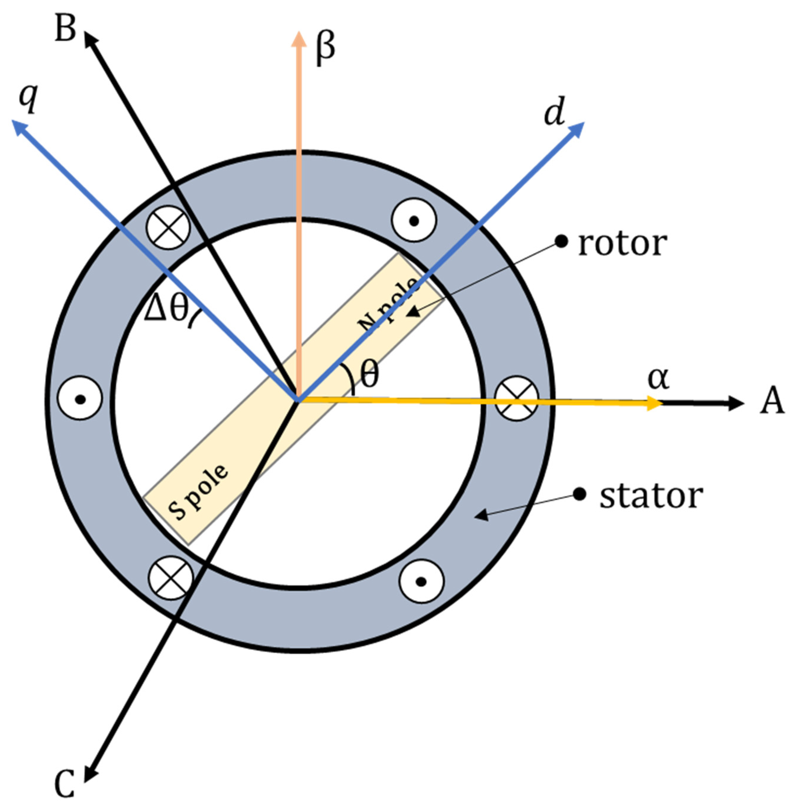
2.1. Mathematical Model of Surface Permanent Magnet Synchronous Motor

PMSM consists of a stator and rotor, using a permanent magnet as excitation instead of field coils, according to the installation site of PM, the motor can divide into surface mounted, embedded, and built-in types. The control circuit inputs a three-phase sinusoidal waveform to the stator of PMSM, and the sinusoidal current is symmetrical. Different from IPMSM, SPMSM has symmetrical air gap magnetic flux, and the inductance at the d-axis and q-axis are equivalent, because of the simple structure and small rotary inertia, it is selected as the object of study. Before establishing the mathematical model of SPMSM, several assumptions are made:

• The study object in this paper is surface-mounted PMSM;
• The waveform of induced electromotive force in the three-phase coil is sinusoidal;
• The electrical conductivity of permanent magnet material is zero;
• The magnetic conductivity inside the permanent magnet is equal to the value in the air;
• Ignoring the core reluctant, eddy-current loss, magnetic hysteresis loss, and core saturation effect.

The Figure 1 shows spatial position relation of the reference frame. Including three-phase stationary coordinate systems, two-phase static coordinate system and two-phase rotation coordinate system. The A axis and $\alpha$ axis located at 0 degrees coincidently. A axis rotates 120 degrees counterclockwise to get B axis, B axis rotates 120 degrees counterclockwise to get C axis. $\alpha$ axis rotates 90 degrees counterclockwise to get $\beta$ axis. The direction of $d$ axis has the same direction as the magnetic poles, and $d$ axis rotates 90 degrees counterclockwise to get $q$ axis.

In the vector control system, the A, B, and C axis, which are also called three-phase stationary coordinate systems, differ 120 electrical degrees from each other, as can be seen in Figure 1, the voltage equation under A, B, and C frame is as follows:

$$\left[\begin{array}{c}{u}_A\\ u_B\\ u_C\end{array}\right]=\left[\begin{array}{ccc}{R}_A+pL& 0& 0\\ 0& R_B+pL& 0\\ 0& 0& R_C+pL\end{array}\right]\left[\begin{array}{c}{i}_A\\ i_B\\ i_C\end{array}\right]-\omega {\psi }_f\left[\begin{array}{c}\sin \theta \\ \sin \left(\theta -\frac{2\pi }{3}\right)\\ \sin \left(\theta +\frac{2\pi }{3}\right)\end{array}\right]$$

(1)

$u_A$, $u_B$, $u_C$ are the voltage of three-phase stator windings, $i_A$, $i_B$, $i_C$ are the current of three-phase stator windings, ${\psi }_A$, ${\psi }_B$, ${\psi }_C$ are the flux linkage of three-phase windings. $R_A$, $R_B$, $R_C$ are the resistances of three-phase stator windings that have the same resistance. Every magnetic flux of stator winding cross-link is equal to the sum of mutual flux and self-induced magnetic flux.

$$L=L_{AA}=L_{BB}=L_{CC}=L_{MN}+L_{LK}$$

(2)

$L_{MN}$ is single-phase magnetic inductance of stator winding, $L_{LK}$ is single-phase leakage inductance.

The flux linkage equation is as follows:

$$\left[\begin{array}{c}{\psi }_A\\ {\psi }_B\\ {\psi }_C\end{array}\right]=\left[\begin{array}{ccc}{L}_{AA}& M_{AB}& M_{AC}\\ M_{BA}& L_{BB}& M_{BC}\\ M_{CA}& M_{CB}& L_{CC}\end{array}\right]\left[\begin{array}{c}{i}_A\\ i_B\\ i_C\end{array}\right]+\left[\begin{array}{c}\cos \theta \\ \cos \left(\theta -\frac{2\pi }{3}\right)\\ \cos \left(\theta -\frac{4\pi }{3}\right)\end{array}\right]{\psi }_f$$

(3)

$L_{AA}$, $L_{BB}$, $L_{CC}$ are the self-inductance of three-phase stator windings ($L_{AA}$= $L_{BB}$= $L_{CC}$ in surface-mounted PMSM); $M_{AB}$, $M_{AC}$, $M_{BA}$, $M_{BC}$, $M_{CA}$, $M_{CB}$ are the mutual inductance of relevant windings, because the relative position of three-phase stator and three phase rotor is fixed, so the mutually inductive of every winding is constant and equal to each other. ${\psi }_f$ is the flux amplitude of the rotor permanent magnet.

The two-phase static coordinate system is α-β frame, as can be seen in Figure 1, the α axis is vertical to the β axis. The three-phase stationary coordinate system transformed into a two-phase stationary coordinate system is always adopted by Clarke transform, the formula follows:

$$\left[\begin{array}{c}{i}_{\alpha }\\ i_{\beta }\end{array}\right]=\sqrt{\frac{2}{3}}\left[\begin{array}{ccc}1& -\frac{1}{2}& -\frac{1}{2}\\ 0& \frac{\sqrt{3}}{2}& -\frac{\sqrt{3}}{2}\end{array}\right]\left[\begin{array}{c}{i}_A\\ i_B\\ i_C\end{array}\right]$$

(4)

The other common coordinate system in vector control system is two-phase rotation coordinate system, which called d-q coordinate system. As can be seen in Figure 1, q axis advance d axis 90 degree. The and the relationship between A, B, C axis and d-q axis are shown as follows:

$$\left[\begin{array}{c}{i}_d\\ i_q\end{array}\right]=\sqrt{\frac{2}{3}}\left[\begin{array}{ccc}\cos \theta & \cos \left(\frac{2}{3}\pi -\theta \right)& \cos \left(\frac{4}{3}\pi -\theta \right)\\ -\sin \theta & \sin \left(\frac{2}{3}\pi -\theta \right)& -\sin \left(\frac{4}{3}\pi -\theta \right)\end{array}\right]\left[\begin{array}{c}{i}_A\\ i_B\\ i_C\end{array}\right]$$

(5)

$d-q$ is the magnetic field-oriented coordinate, $d$ axis is a coincidence with the magnet pole axis of the rotor, and $q$ axis is 90° ahead of the d axis counterclockwise. The state equation under the d-q coordinate system of surface permanent magnet synchronic motor is:

$$\{\begin{array}{c}{u}_d=p{\Psi }_d-{\omega }_e{\Psi }_q+R{i}_d\\ u_q=p{\Psi }_q+{\omega }_e{\Psi }_d+R{i}_q\end{array}$$

(6)

The flux linkage equation is as follows:

$$\{\begin{array}{c}{\Psi }_d=L_d{i}_d+{\Psi }_f\\ {\Psi }_q=L_q{i}_q\end{array}$$

(7)

The equation of electronic torque is:

$$T_e=\frac{3}{2}{p}_n{\psi }_f{i}_q$$

(8)

The equation of rotor mechanism motion is:

$$J\frac{d{\omega }_r}{dt}=T_e-T_L-B{\omega }_r$$

(9)

where $i_d$, $i_q$ are the currents of the d and q axis, respectively, and consist of stator current; $u_d$, $u_q$ are the voltage of the d and q axis, respectively, which consist of stator voltage; $R_s$, $L_s$ is resistance and inductance of stator windings; $p$ is the differential operator with respect to time $t$. $p_n$ is the number of pole pairs; ${\psi }_f$ is rotor flux linkage; $T_e$ is the electromagnetic torque; $T_L$ is load torque; ${\omega }_e$ is electronic angle speed; ${\omega }_r$ is the mechanical angle speed of the rotor. B is the damping factor; J is the moment of inertia.

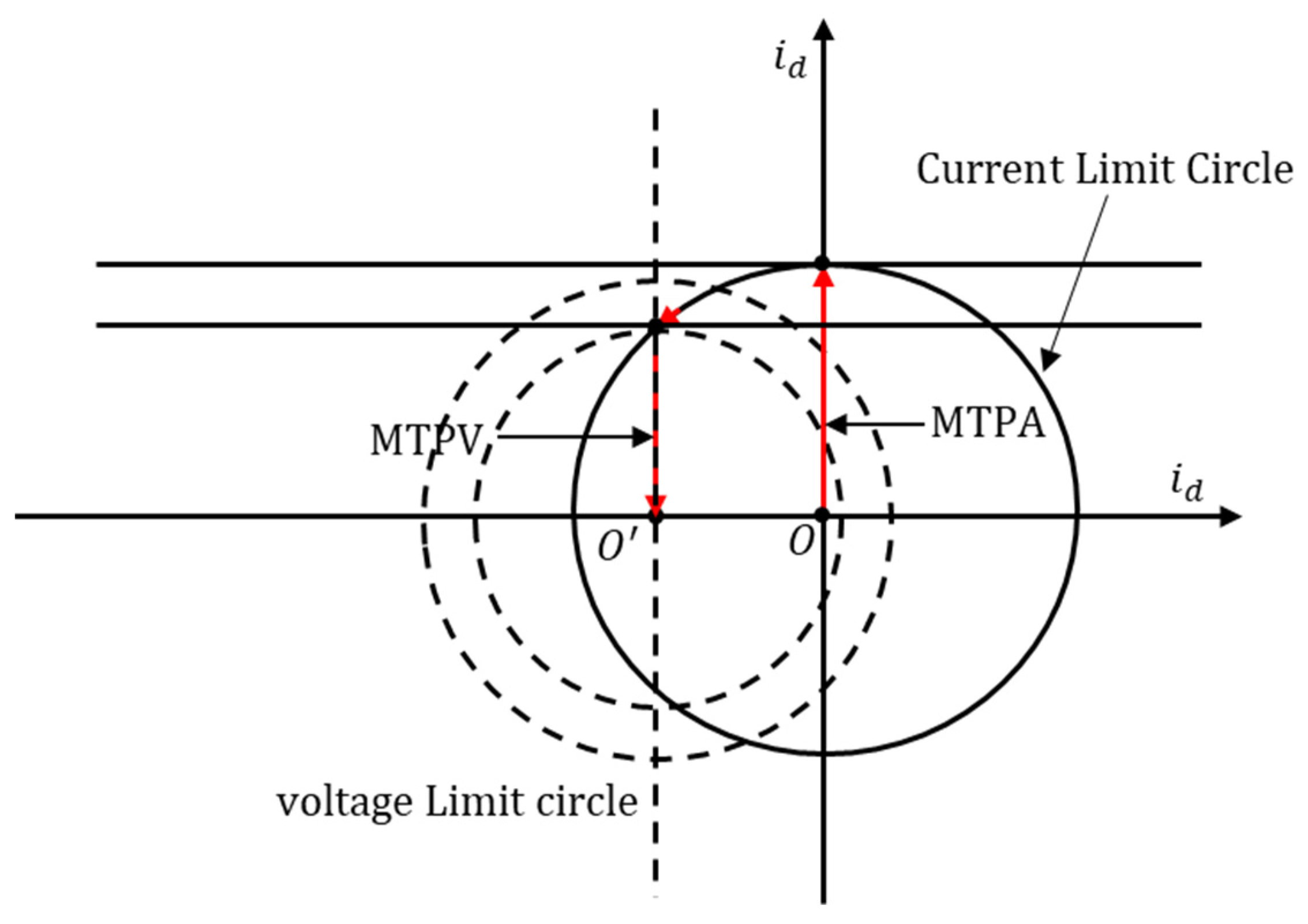
2.2. SPMSM Sensorless Control Technique in High Speed Region

In the vector control system, the output of the inverter has the highest limit value, for the limitation of dc bus voltage and dc bus utilization of inverter, the value of inverter space voltage vector and space current vectors have a maximum value. The voltage limit circle equation can be expressed as:

$${\left(i_d+\frac{{\Psi }_f}{L_d}\right)}^2+p^2{i}_q^2={\left(\frac{u_{smax}}{{\omega }_e{L}_d}\right)}^2$$

(10)

In the equation, $p$ is the salient pole rate, meet the condition: $p=\frac{L_q}{L_d}$. $u_{smax}$ is the current limit value, $u_s$ is the amplitude of voltage vector, the relationship between variables meets the condition:

$$u_s=\sqrt{u_d^2+u_q^2}\le u_{smax}$$

(11)

When PMSM steady operation in flux weakening region, the voltage drop in stator resistance can be ignored, the equation of stator voltage is:

$$\{\begin{array}{c}{u}_d=-{\omega }_e{L}_q{i}_q\\ u_q={\omega }_e{L}_d{i}_d+{\omega }_e{\Psi }_f\end{array}$$

(12)

According to the above equations, the rotation speed expression is obtained:

$${\omega }_{emax}\leqq \frac{u_{smax}}{\sqrt{{\left(L_d{i}_d+{\Psi }_f\right)}^2+{\left(L_q{i}_q\right)}^2}}$$

(13)

From the relationship equation of rotation speed, reducing the current of the d or q axis will contribute to improving the speed of PMSM.

For SPMSM, because the d and q axis inductance is equal to each other: $L_d=L_q=L_s$, corresponding to $p=1$, so the voltage limit circle is a perfect circle, and the coordinate of this circle is $(-\frac{{\Psi }_f}{L_s},0)$, the radius of this circle is $\frac{u_s}{{\omega }_e{L}_s}$, within the voltage limit circle, if the electronic speed ${\omega }_e$ is constantly, when improving the value of stator voltage, the voltage limit circle will outward spreading; if the electronic speed ${\omega }_e$ improved, the voltage limit circle will contract towards the center.

When the voltage limit $u_{smax}$, current limit $i_{smax}$ is decided, the flux weakening performance of SPMSM is affected by d and q axis inductance $L_d$, $L_q$ and permanent magnet flux linkage ${\Psi }_f$. The main methodology of flux weakening control is to coordinate transformation and implement the d-q axis current independent control. The excitation flux linkage is provided by a permanent magnet, in order to weaken the air-gap flux, increasing the demagnetization current $i_d$ is the only way to accomplish it, and finally achieve the goal of speed expansion.

According to the steady-state operating characteristic of PMSM, for a certain electromagnetic torque, there exist one work point that the motor has minimum current amplitude when output same torque and MTPA curve is the quadrature axis component of stator current under d-q reference frame. When the motor operates in a high-speed region, one certain electromagnetic torque corresponding to a minimum stator voltage, the MTPV curve is the quadrature axis component of stator voltage. Each point on the curve of MPTV is the maximum torque that the motor can output at the corresponding speed at that point.

As can be seen in Figure 2 that the operation curve of SPMSM can be roughly divided into three regions. In the first region, the maximum torque per ampere(MTPA) method is adopted, letting SPMSM output maximum torque. In the second region, the speed is limited by the effect of voltage and current limit circle, the trajectory coincides with the current limit circle. In the third region, the speed is higher than ever before, and the operation is only affected by voltage limit circle, maximum torque per voltage(MTPV) method is adopted, in this region, the characteristic current is higher than current limitation.

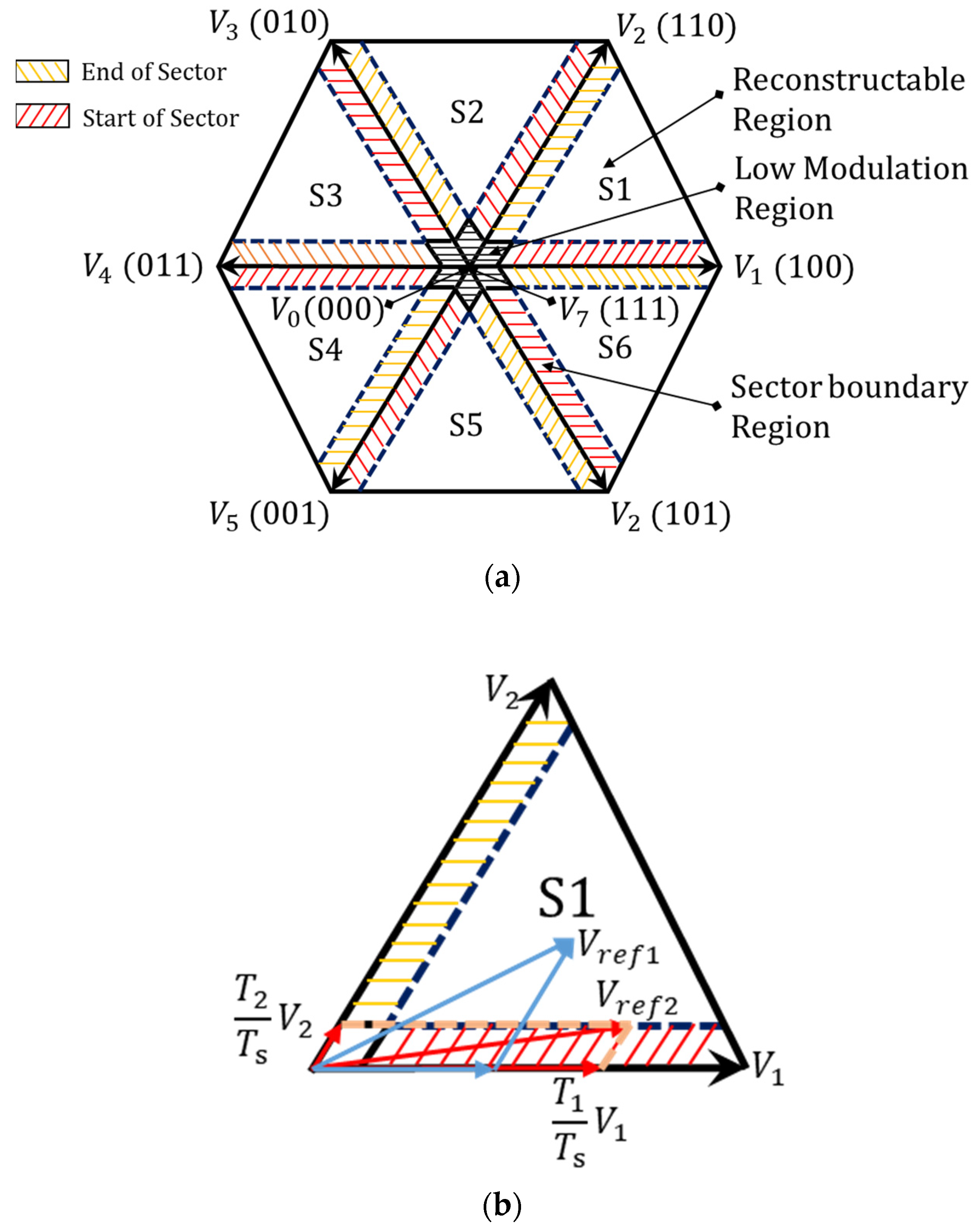
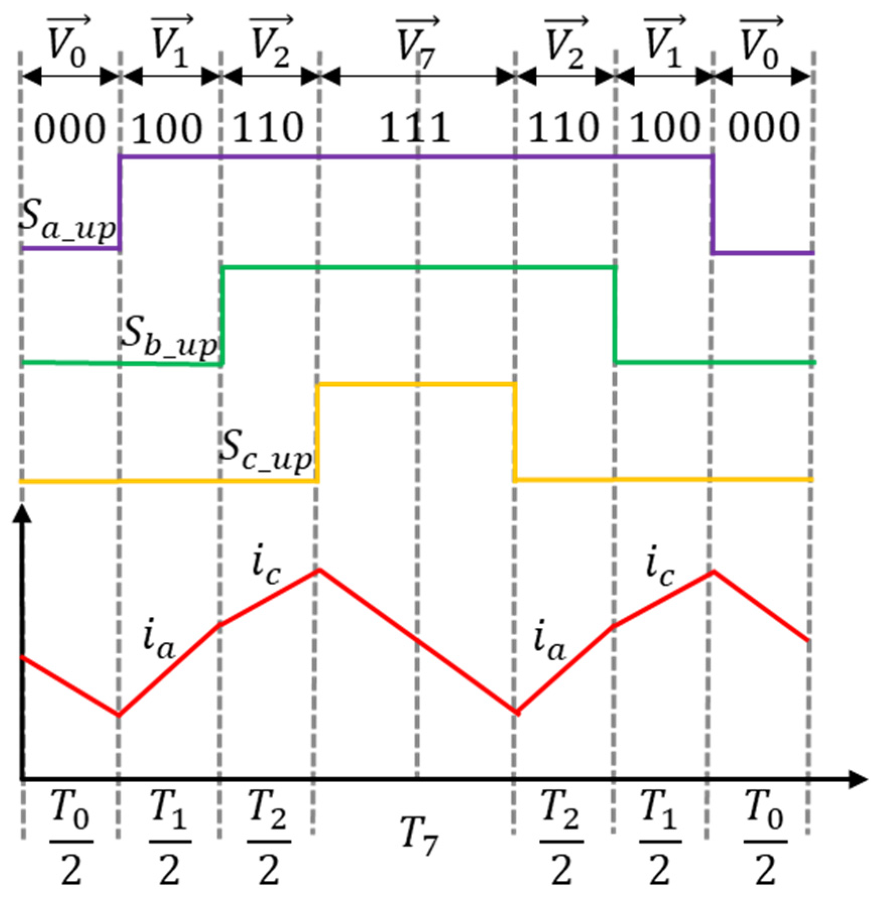
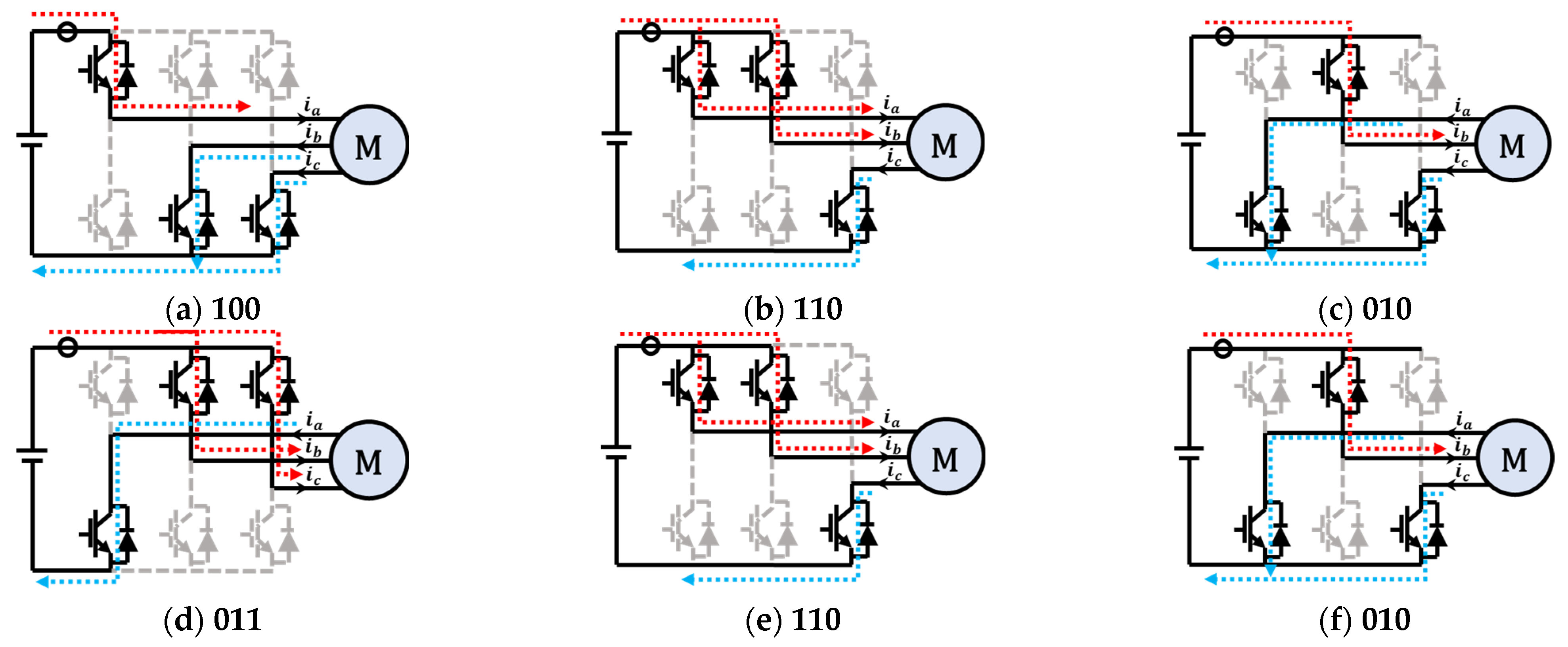
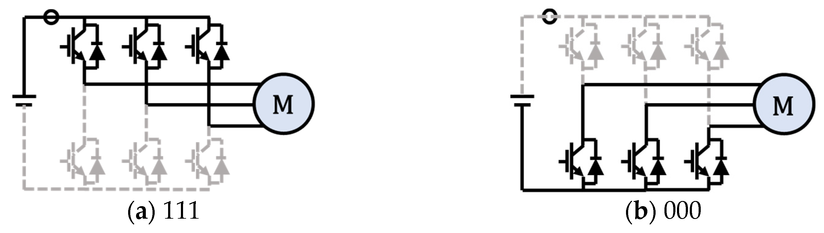
3. Current Reconstruction Methods Using Single Resistance Sensor

The three-phase full-bridge voltage source inverter is the most common circuit topology used for driving three-phase permanent magnet synchronous motors. In this structure, phase current is usually collected with two- or three-phase current sensors, but the current branch usually contains information about the winding phase current, so three-phase current can be reconstructed by only one current sensor.

There are eight space voltage vectors based on different switch states of the inverter, as shown in Figure 2, assuming the direction of current flowing into the motor is positive and the direction of current flowing out of the motor is negative, six of the vectors are nonzero voltage vectors, and two of them are zero voltage vectors. Multiple switch combinations made the branch current between any two power tubes will change with the switching states, based on the different phase current information, phase current can be reconstructable. Every nonzero voltage vector has two sector boundary regions and one reconstructable region. The corresponding relationship between each branch current and winding phase current is shown in

Table 1. The relationship between dc-link current and voltage vectors.

Voltage Vector	Up Switches	${\mathit{i}}_{\mathit{d}\mathit{c}}$
$\stackrel{\rightharpoonup }{V_0}$	000	0
$\stackrel{\rightharpoonup }{V_1}$	100	$i_a$
$\stackrel{\rightharpoonup }{V_2}$	110	$-i_c$
$\stackrel{\rightharpoonup }{V_3}$	010	$i_b$
$\stackrel{\rightharpoonup }{V_4}$	011	$-i_a$
$\stackrel{\rightharpoonup }{V_5}$	001	$i_c$
$\stackrel{\rightharpoonup }{V_6}$	101	$-i_b$
$\stackrel{\rightharpoonup }{V_7}$	111	0

. It can be seen from the table that the current of each branch of the inverter changes with the change of switching state and contains different phase current information.

A novel method is to insert zero voltage vectors at the beginning and the end of a PWM period, respectively. As shown in Figure 3, The zero vector $V_0$ and $V_7$ are inserted at the middle time and the start and end time of each PWM cycle. The rest part is made up of effective voltage vectors. When sampling for a single current sensor at a different time on a PWM cycle, it will sample two different phase currents under two different voltage vectors, then, the third phase current can be calculated. In the actual motor control system, sample process, switch process, and analog to digital conversion time cannot be ignored, in order to achieve stable current sampling, the working time of effective vectors must be longer than the minimum sampling time $T_{min}$. The relationship of time factors is as follows:

$$T_{min}=T_d+T_{set}+T_{con}$$

(14)

$T_d$ expresses the time of deadzone, $T_{set}$ is the duration of the transient process during state change of switch tube, $T_{con}$ is the total time required by a microprocessor sampling module from sampling to converting analog to digital quantities. The minimum sampling time made non-sampling area originated from a novel SVPWM modulation strategy, the sector boundary region is corresponding to the non-sampling area, in this area, phase current information cannot be sampled.

Figure 4 shows the seven segment PWM waveform of SVPWM algorithm based on Figure 3. During one period, the reference voltage vectors are applied according to this order: $\overrightarrow{V_0}$, $\overrightarrow{V_1}$, $\overrightarrow{V_2}$, $\overrightarrow{V_7}$, $\overrightarrow{V_2}$, $\overrightarrow{V_1}$, $\overrightarrow{V_0}$. The waveform is symmetric.

Current flow paths under different vectors are shown in Figure 5 and Figure 6. $S_i$ means the switching state of three phase power electronic device, when $S_i=0$, the low switch of i phase is turn on while the high switch is turn out, on the contrary, when $S_i=1$, the high switch of i phase is turn on while the low switch is turn out.

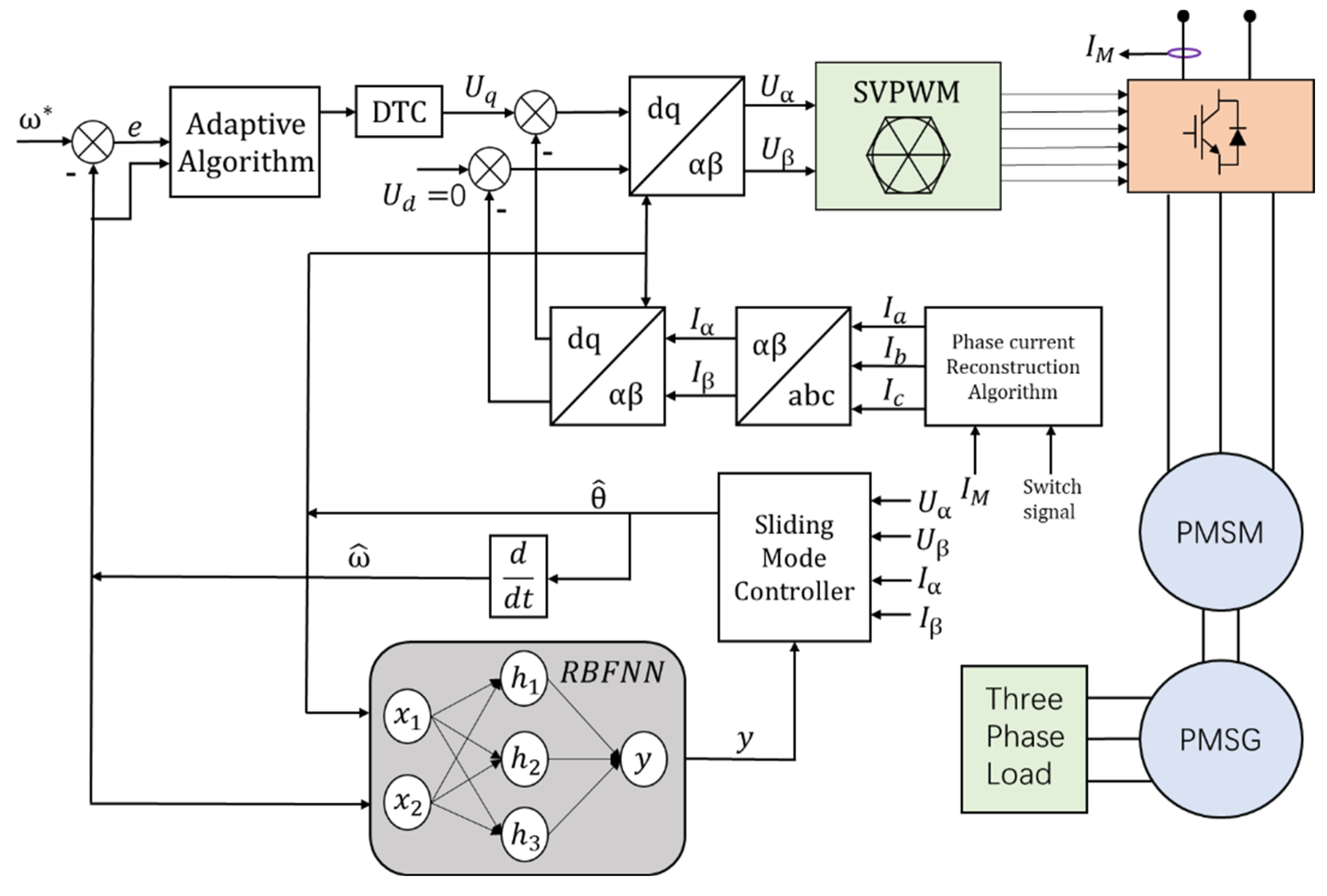
4. Sensorless Control Technique Using Terminal Sliding Mode Controller and RBF Neural Network

4.1. Adaptive Terminal Sliding Mode Control Method

Reasonable sliding mode control law can improve the convergence characteristics of the control system. The sliding switching surface mainly includes linear sliding mode and terminal sliding mode. The system state trajectory of the linear sliding mode can keep closer to the given trajectory, but cannot find the given trajectory during a finite time.

Terminal sliding mode control adapts nonlinear methods, so it has no connection with the statement of the system, by means of optimizing the switching rules, system systematic state variables will converge to the desired point of the system control according to the designed sliding modes in limit time. Under terminal sliding mode control, both the uncertainty of system parameters and the uncertainty of external disturbance have robust performance. This paper proposes an optimized terminal sliding mode, this control law combines exponential reaching law with power reaching law, and it also introduces a new adaptive coefficient to improve the approaching rate. The optimal method overcomes the disadvantages of novel sliding mode methods such as slow approaching rate and the chattering performance in a singular point.

If $x_{d }\left(t\right)$ is reference trajectory, the tracking error is:

$$e\left(t\right)=\theta \left(t\right)-{\theta }_d\left(t\right)$$

(15)

So, the velocity estimation error of the control system is:

$$\dot{e}\left(t\right)=\dot{\theta }\left(t\right)-{\dot{\theta }}_d\left(t\right)$$

(16)

$$\ddot{e}\left(t\right)=\ddot{\theta }\left(t\right)-{\ddot{\theta }}_d\left(t\right)$$

(17)

Constructing the sliding mode surface of displacement stage is as follows:

$$S=c_{1}e+c_2\dot{e}$$

(18)

$$\dot{S}=c_1\dot{e}+c_2\ddot{e}$$

(19)

In order to eliminate the effectiveness of sliding mode chattering, a continuous saturation function is put forward instead of a sign function:

$$sat\left(s\right)=\{\begin{array}{c}1 (s>\epsilon )\\ \frac{s}{\epsilon } \left(\left|s\right|\le \epsilon \right)\\ -1 (s<\epsilon )\end{array}$$

(20)

Adopting exponential convergence law based on saturation function as sliding mode control law:

$$\dot{S}=-\epsilon s sat\left(s\right)-ks\hspace{1em}\hspace{1em}\hspace{1em}\hspace{1em}(\epsilon >0, k>0)$$

(21)

The terminal sliding mode surface of the above system can be expressed as:

$$S=e+\beta {\left|e\right|}^{\frac{p}{q}}sat\left(s\right)+\lambda e^m$$

(22)

In the above equation, $\beta >0$, $\lambda >0$, both $p$ and $q$ are odd numbers, and the relationship between them satisfies: $0<q<p$, $m>1$.

Selecting the control law is:

$$i\left(t\right)=i_{eq}\left(t\right)+i_{sw}\left(t\right)$$

(23)

In the equation, $u_{eq}\left(t\right)$ is equivalent control part, $u_n\left(t\right)$ is the nonlinear control part, set equivalent controller part:

$$i_{eq}\left(t\right)=\frac{J}{P_n{\Psi }_f}\left(\frac{B{\omega }_r}{J}+\frac{\beta p}{q}{e}^{\frac{q}{p}-1}\dot{e}+\alpha \dot{e}\right)$$

(24)

Set nonlinear controller part:

$$i_{sw}\left(t\right)=ks+\eta e^{\frac{q}{p}}sat\left(s\right)$$

(25)

According to the designed control law, infinite control output exists in any region of system state variables, and the singularity problem is also non-existent. The statement of the system will converge to the terminal sliding surface for a limited time.

Consider the Lyapunov function:

$$V\left(x\right)=\frac{1}{2}{S}^{T}S=\frac{1}{2}{S}^2$$

(26)

According to the Lyapunov method, the reachability condition of sliding mode control is:

$$\dot{V\left(x\right)}=\dot{S}S<0$$

(27)

If Lyapunov function $V\left(x\right)=\frac{1}{2}{S}^2$ meets the condition:

$$\dot{V}\left(S\right)+\alpha V\left(S\right)+\beta V^{\gamma }\left(S\right)\le 0(\alpha ,\beta >0, 0<\gamma <0)$$

(28)

$S$ will converge to zero in a limited time, and the converge time is

$$T\le \frac{1}{\alpha \left(1-\gamma \right)}\ln \frac{\alpha V^{1-\gamma }\left(S_0\right)+\beta }{\beta }$$

(29)

Derivative the terminal sliding mode function, we can conclude that:

$$\dot{S}=\dot{e}+\beta \frac{p}{q}{\left|\dot{e}\right|}^{\frac{p}{q}-1}sat\left(S\right)+m\lambda e^{m-1}\dot{e}$$

(30)

$$\begin{gathered} V=S\dot{S} \\ =S\left(\dot{e}+\beta \frac{p}{q}{\left|\dot{e}\right|}^{\frac{p}{q}-1}\ddot{e}+m\lambda e^{m-1}\dot{e}\right) \\ =S(\dot{e}+\beta \frac{p}{q}{\left|\dot{e}\right|}^{\frac{p}{q}-1}\left(\ddot{\theta }\left(t\right)-{\ddot{\theta }}_d\left(t\right)\right)+m\lambda e^{m-1}\dot{e}) \end{gathered}$$

(31)

$${\omega }^{*}={\displaystyle \int }\left[\ddot{\theta }\left(t\right)+{\beta }^{-1}{\left(\frac{p}{q}\right)}^{-1}{\left|\dot{e}\right|}^{2-\frac{p}{q}}sat\left(\dot{e}\right)+m^{-1}\lambda e^{2-m}sat\left(\dot{e}\right)+\epsilon s sat\left(s\right)+ks\right]d\tau$$

(32)

$$\begin{gathered} \dot{V}=S\left[\left(-\frac{p}{q}{\left|\dot{e}\right|}^{\frac{p}{q}-1}-m\lambda e^{m-1}\right)\left(\epsilon s^{\rho }sat\left(s\right)+ks\right)\right] \\ \leqq -\epsilon s^{\rho +1}-ks \\ \leqq -2^{\frac{\rho +1}{2}}k{V}^{\frac{\rho +1}{2}}-2kV \end{gathered}$$

(33)

$$k=min\{\frac{{\left|\dot{e}\right|}^{\frac{p}{q}-1}}{\beta \frac{p}{q}}k\}$$

According to the above, the terminal sliding mode control system will converge to the sliding mode manifold, and the state variables will also converge to zero for a limited time.

4.2. Design of Terminal Adaptive Sliding Mode Controller Based on RBF Neural Network

A radial basis function neural network is introduced to solve the chattering problem of the conventional sliding mode manifold. The main objective of the radial basis function is used for the prediction of back-EMF. The compensation for the RBF network’s approximate error is the switch function of sliding mode control. The Figure 7 shows the structure diagram of adaptive sliding mode control using RBF neural network in a sensorless servo system. The input of phase current reconstruction algorithm is measured current value and switch signal, and reconstruct three phase current. The inverse Clark transformation block and inverse Parker transformation provide $U_{\alpha }$, $U_{\beta }$, $I_{\alpha }$, $I_{\beta }$ to sliding mode controller to estimate the value of angle. RBFNN part capture the current value of angle and angular velocity, and feedback the trained value to the sliding mode controller.

$$u={\displaystyle \sum }_{j=1}^m{w}_j\exp \left(-\frac{{\left|\left|X-C_j\right|\right|}^2}{2b_j^2}\right)$$

(34)

Where $C_j=\left[C_{j1},C_{j2},\dots ,C_{jn}\right]$ is the center vector value of the jth hidden layer neuron. X is the input value of the network. Let the weight vector of the network in the hidden layer be: $W={\left[\begin{array}{cc}{w}_1& w_2\end{array}\cdots w_j\cdots w_m\right]}^T$, the base width vector of the network is setting: $B={\left[\begin{array}{cc}{b}_1& b_2\end{array}\cdots b_m\right]}^T$, $b_m$ is the $mth$ base width parameter.

The output function of the radial basis function neural network is

$${\widehat{f}}_i=W_i^T{h}_i\left(x_i\right), i=1,2,\dots ,n$$

(35)

The predicted output of the neural network is:

$$f_i=W_i^{*T}{h}_i\left(x_i\right)+\mathsf{\Delta }, i=1,2,\dots ,n$$

(36)

$\mathsf{\Delta }$ means the predicted error of the neural network. Define ${\tilde{W}}_i$ is weight estimation error:

$${\tilde{W}}_i=W_i^{*}-{\widehat{W}}_i^{*}$$

(37)

Define $\tilde{d}$ is interference prediction error, the relationship meeting:

$${\tilde{f}}_i=f_i-{\widehat{f}}_i$$

(38)

The output of the network discriminator is:

$$J_{out}=\frac{1}{2}{\left(y_{out}\left(k\right)-y_m\left(k\right)\right)}^2$$

(39)

In the above equation, $y_{out}\left(k\right)$ is the output of the servo system, $y_m\left(k\right)$ is the output of the neural network.

According to gradient descent, the iterative algorithm of the network’s parameter can be worked out such as node center, output weight, and the parameter of node base width. The updated weights:

$$\{\begin{array}{c}{w}_j\left(k\right)=w_j\left(k-1\right)+\eta \left(y_{out}\left(k\right)-y_m\left(k\right)\right)h_j+\alpha \left(w_j\left(k-1\right)-w_j\left(k-2\right)\right)\\ \mathsf{\Delta }{w}_j\left(k\right)=\eta \left(y_{out}\left(k\right)-y_m\left(k\right)\right)h_j\end{array}$$

(40)

The updated base width parameter:

$$\{\begin{array}{c}{b}_j\left(k\right)=b_j\left(k-1\right)+\eta \mathsf{\Delta }{b}_j+\alpha \left(b_j\left(k-1\right)-b_j\left(k-2\right)\right)\\ \mathsf{\Delta }{b}_j\left(k\right)=\left(y_{out}\left(k\right)-y_m\left(k\right)\right)w_j{h}_j\frac{\left|\left|X-C_j\right|\right|}{b_j^3}\end{array}$$

(41)

The updated hidden layer:

$$\{\begin{array}{c}{c}_{ji}\left(k\right)=c_{ji}\left(k-1\right)+\eta \mathsf{\Delta }{c}_{ji}+\alpha \left(c_{ji}\left(k-1\right)-c_{ji}\left(k-2\right)\right)\\ \mathsf{\Delta }{c}_{ji}\left(k\right)=\left(y_{out}\left(k\right)-y_m\left(k\right)\right)w_j\frac{X-C_{ji}}{b_j^2}\end{array}$$

(42)

In this equation, $\alpha$($0<\alpha <1$) is the factor of momentum, $\eta$ ($0<\eta <1$) is the learning rate. In order to detect the input and output of the controlled system, the momentum term t can play a damping role in adjusting the parameters, represents the previously accumulated adjustment effect, can better maintain the stability of the system, and improve training speed degree.

The Lyapunov function is designed as:

$$V=\frac{1}{2}{S}^2+\frac{1}{2}{\eta }^{-1}{\tilde{W}}^T\tilde{W}$$

(43)

$\tilde{W}=W^{*}-\widehat{W}, \dot{\widehat{W}}=-\dot{\widehat{W}}.$ Take derivation of the above equation with respect to time:

$$\begin{gathered} \dot{V}=S^T\dot{S}+{\eta }^{-1}{\tilde{W}}^T{\dot{\widehat{W}}}^{*} \\ =s(-\epsilon ssat\left(s\right)-ks+\mathsf{\Delta })+{\widehat{W}}^T(sh\left(s\right)-\eta {\dot{\widehat{W}}}^{*}) \end{gathered}$$

(44)

Selecting adaptive law:

$${\dot{\widehat{W}}}^{*}=\frac{1}{\eta }sh\left(s\right)$$

(45)

$$\dot{V}=-\epsilon s^{2}sat\left(s\right)-\left(k{s}^2-\mathsf{\Delta }\right)-k{s}^2\leqq 0$$

(46)

When $k{s}^2>0$, can ensure: $\dot{V}\leqq -k{s}^2\leqq 0$. Assumed a function:

$$D\left(t\right)=-k{t}^2$$

(47)

It can be concluded that: $\underset{t\to \infty }{\lim }D\left(t\right)=0$

When time is close to infinite, the system error is close to zero, which verifies the stability of the system.

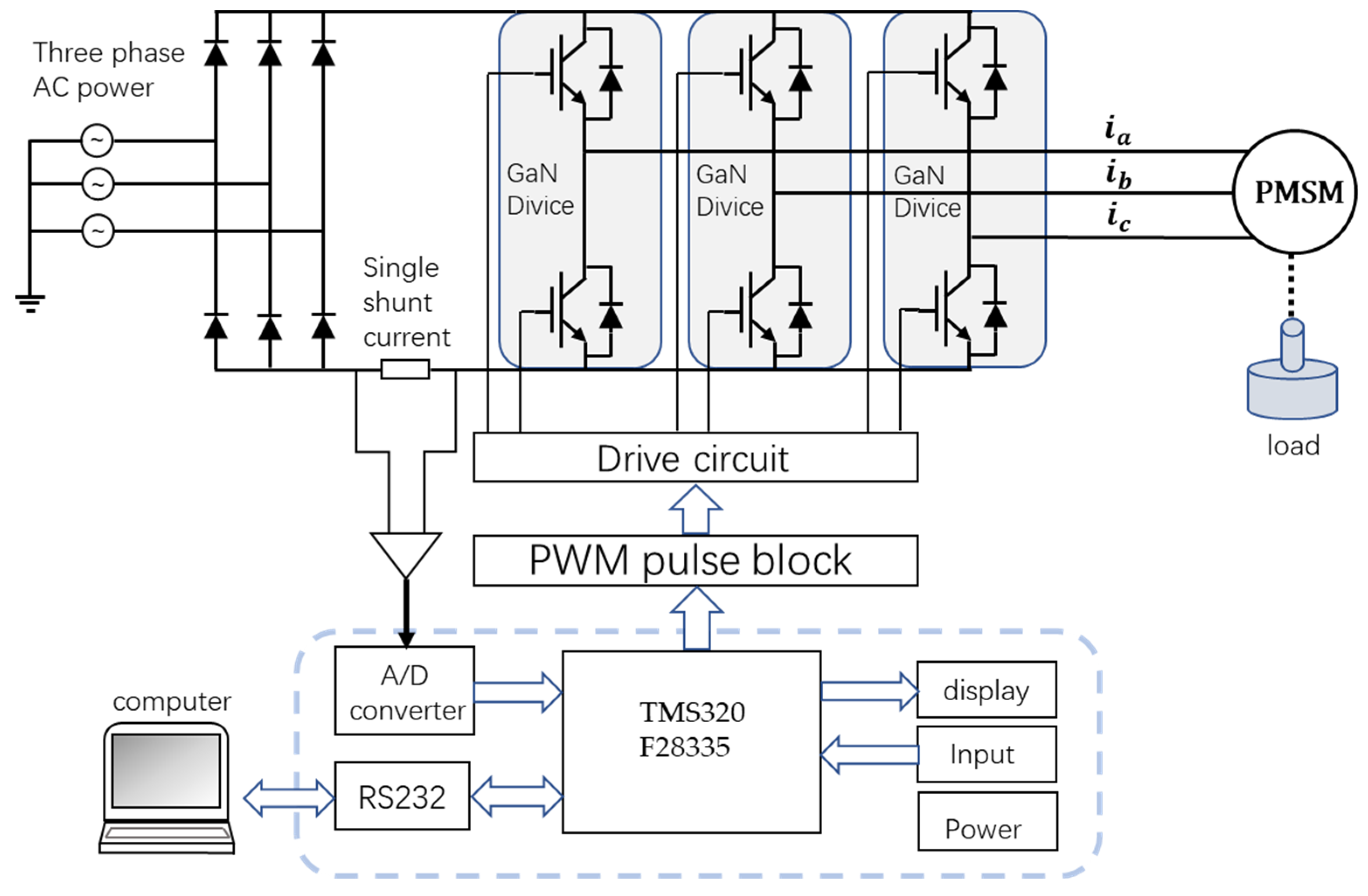
5. Hardware Design of Control System

To verify the proposed adaptive terminal sliding mode RBF neural network control method for SPMSM control, the hardware of the ac servo drive system is established. The structure diagram can be seen in Figure 8, the hardware including TMS320F28335 main control unit, PWM pulse block, drive circuit, GaN devices and upper computer. The real image of the hardware under test can be seen in Figure 9.

6. Simulation and Experiment Verification

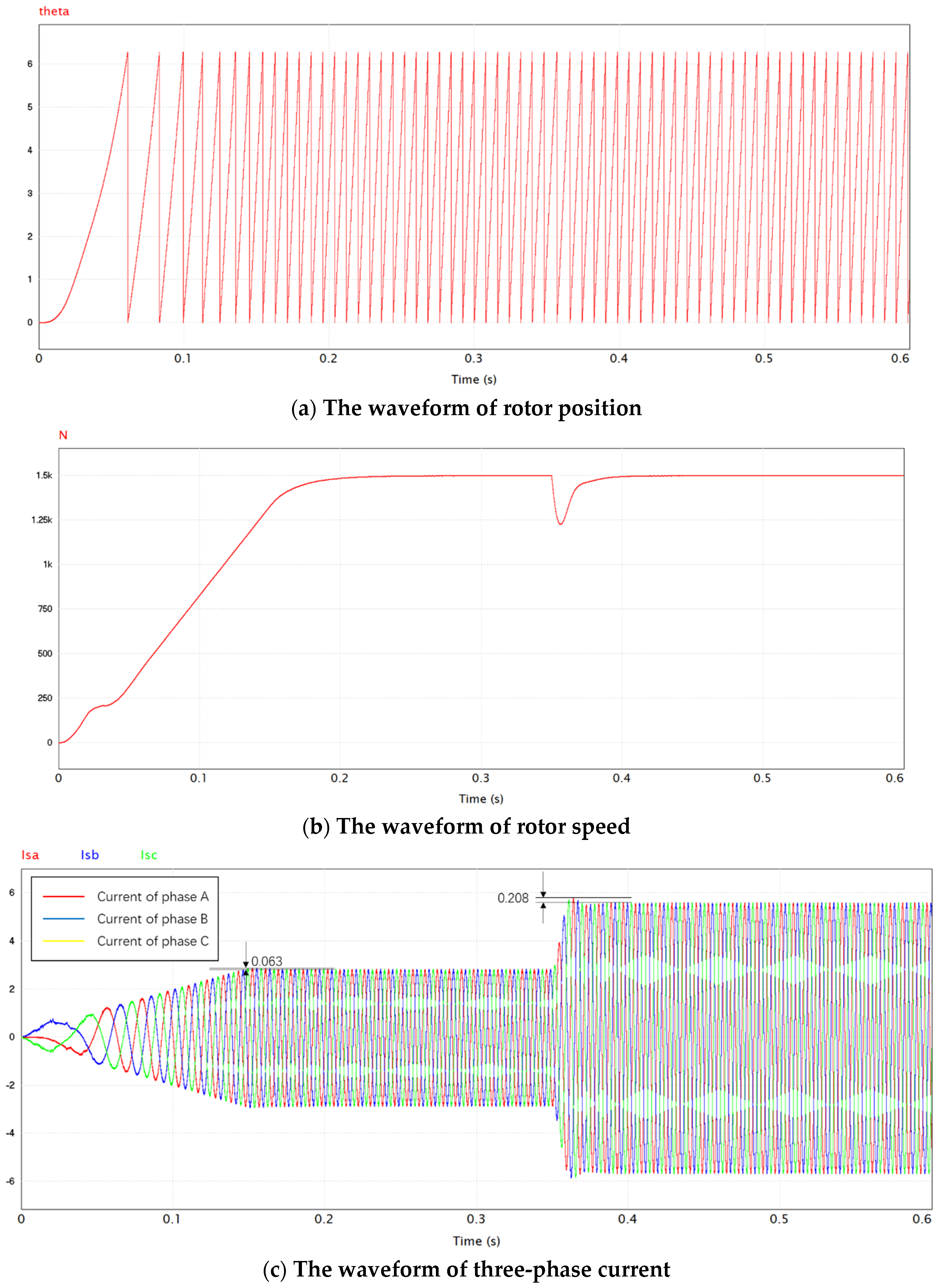
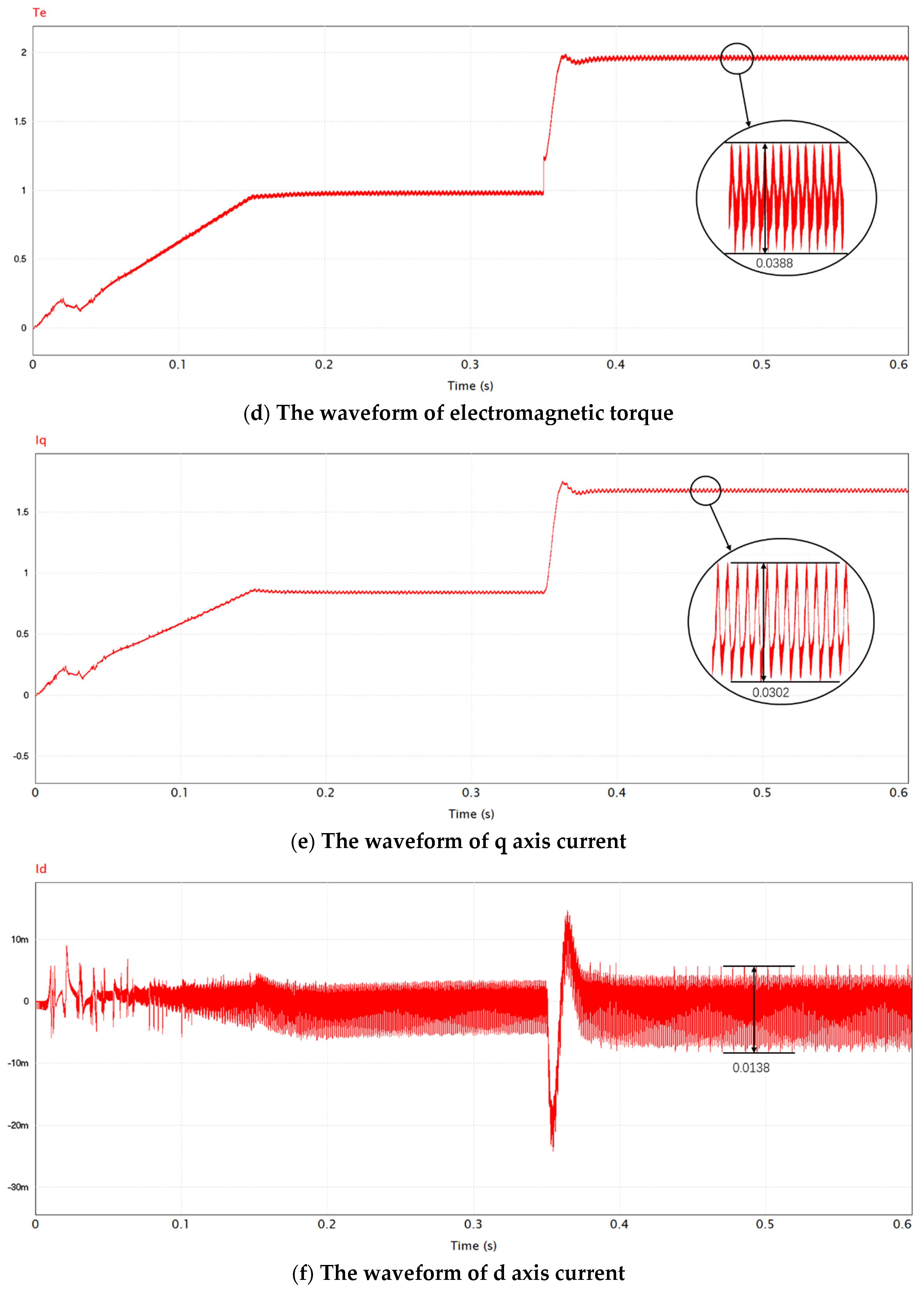
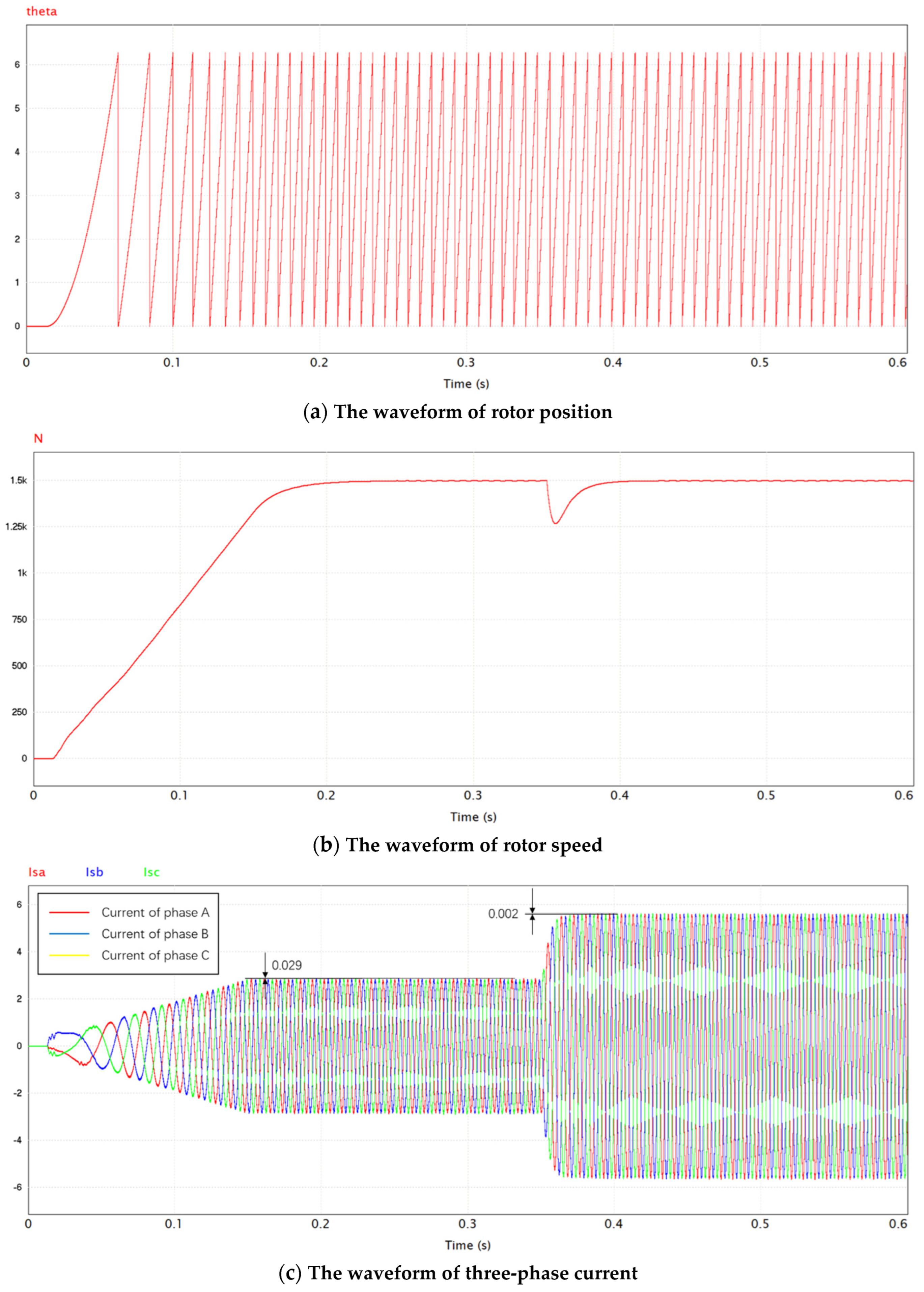
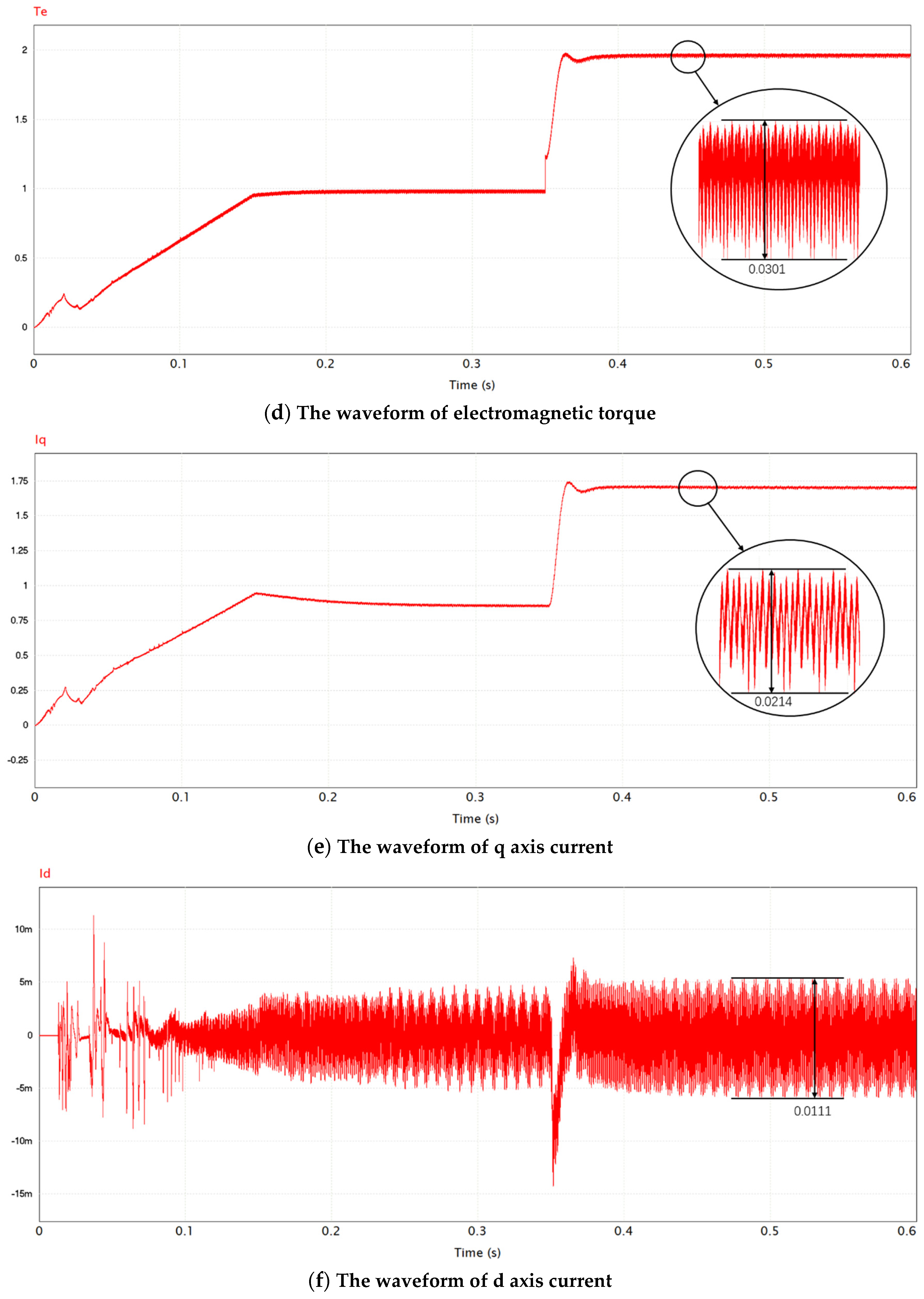
6.1. Simulation Results

In this section, the power simulation software is used to simulate control methods for surface permanent magnet synchronic motors.

As can be seen, Figure 10 shows the simulation result of conventional sliding mode control, Figure 11 shows the simulation control of RBF neural network sliding mode control, and Figure 12 shows the simulation results of adaptive RBF neural network sliding mode control, which includes rotor position waveform, speed waveform, three-phase current waveform, electromagnetic torque waveform, and the current waveform of the d and q axis. A load is added in 0.35 s in the simulation. Comparing the three groups of data, the conventional SMC can obtain the real-time performance the same as the other two groups, but the overshoot is higher than others. The overshoot after adding load in Figure 10 is 0.208 V, in Figure 11, the overshoot value after adding load is down to 0.105 V, this value in Figure 12 is down to 0.002V. The wave range of conventional sliding mode control method and RBF neural network sliding mode control method of torque and d q current is also wider in Figure 11 and Figure 12. However, the adaptive RBFNN-SMC method can track reference rotor speed rapidly without overshoot in Figure 12, and the dynamic performance after adding load is also transit smoothly.

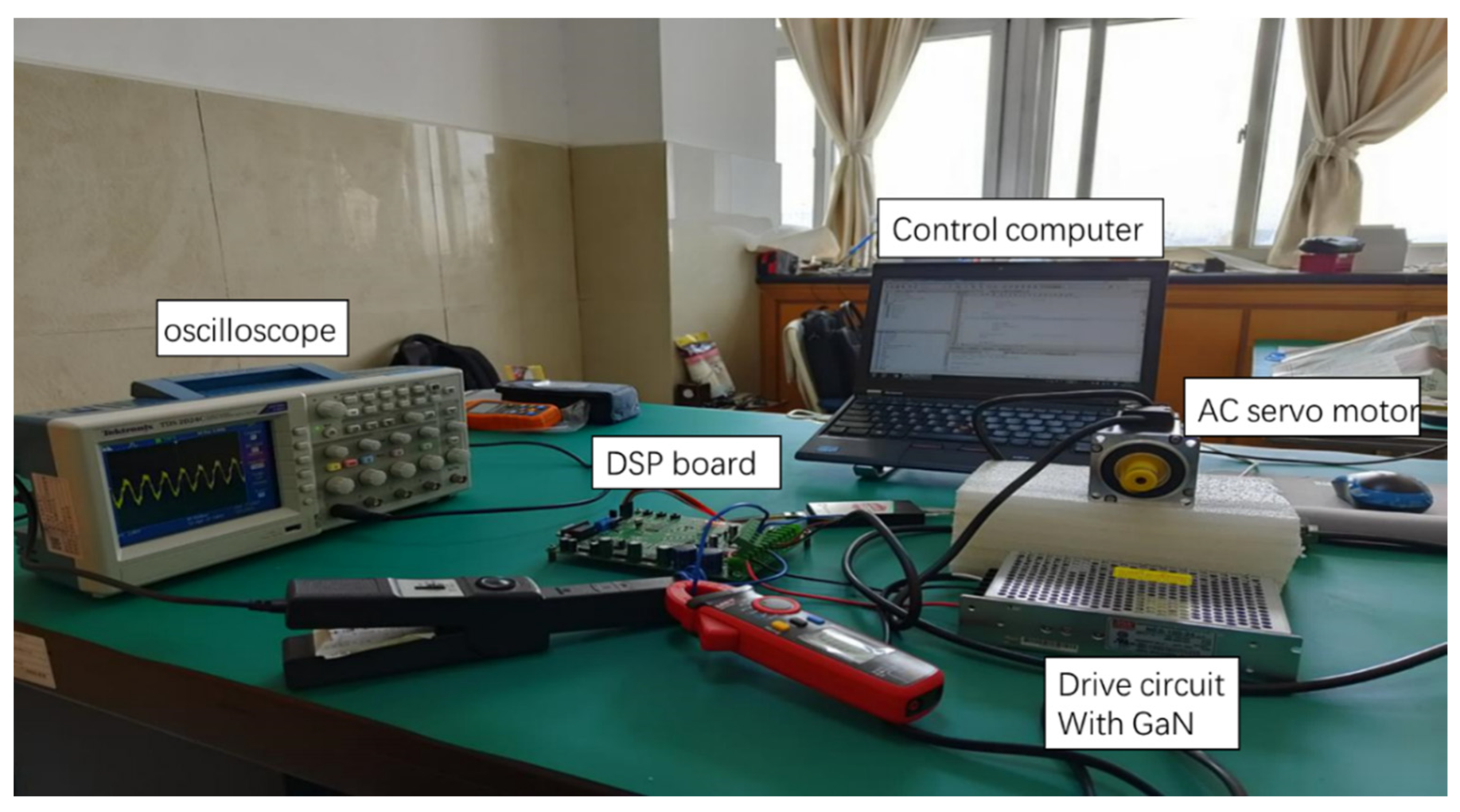
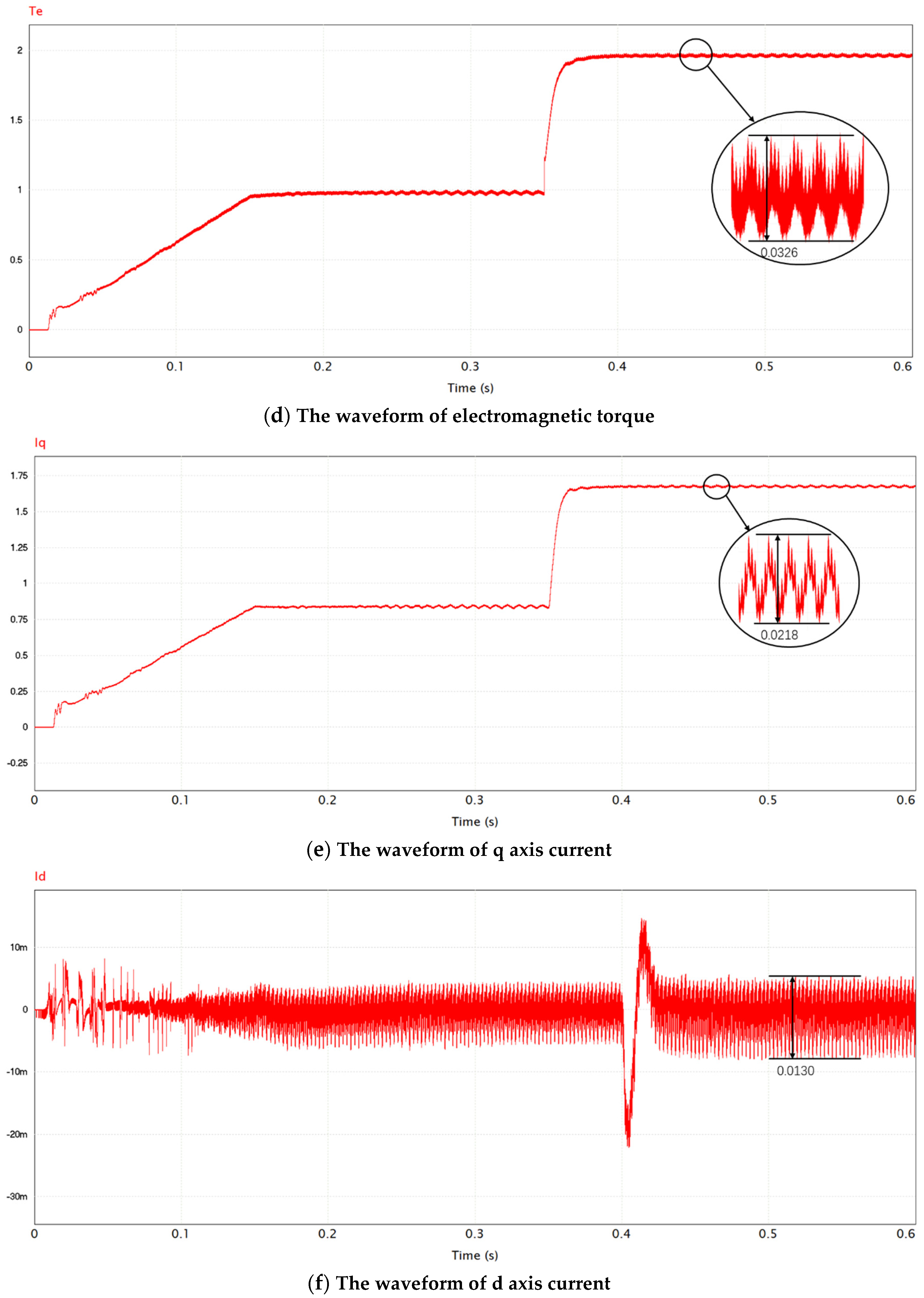
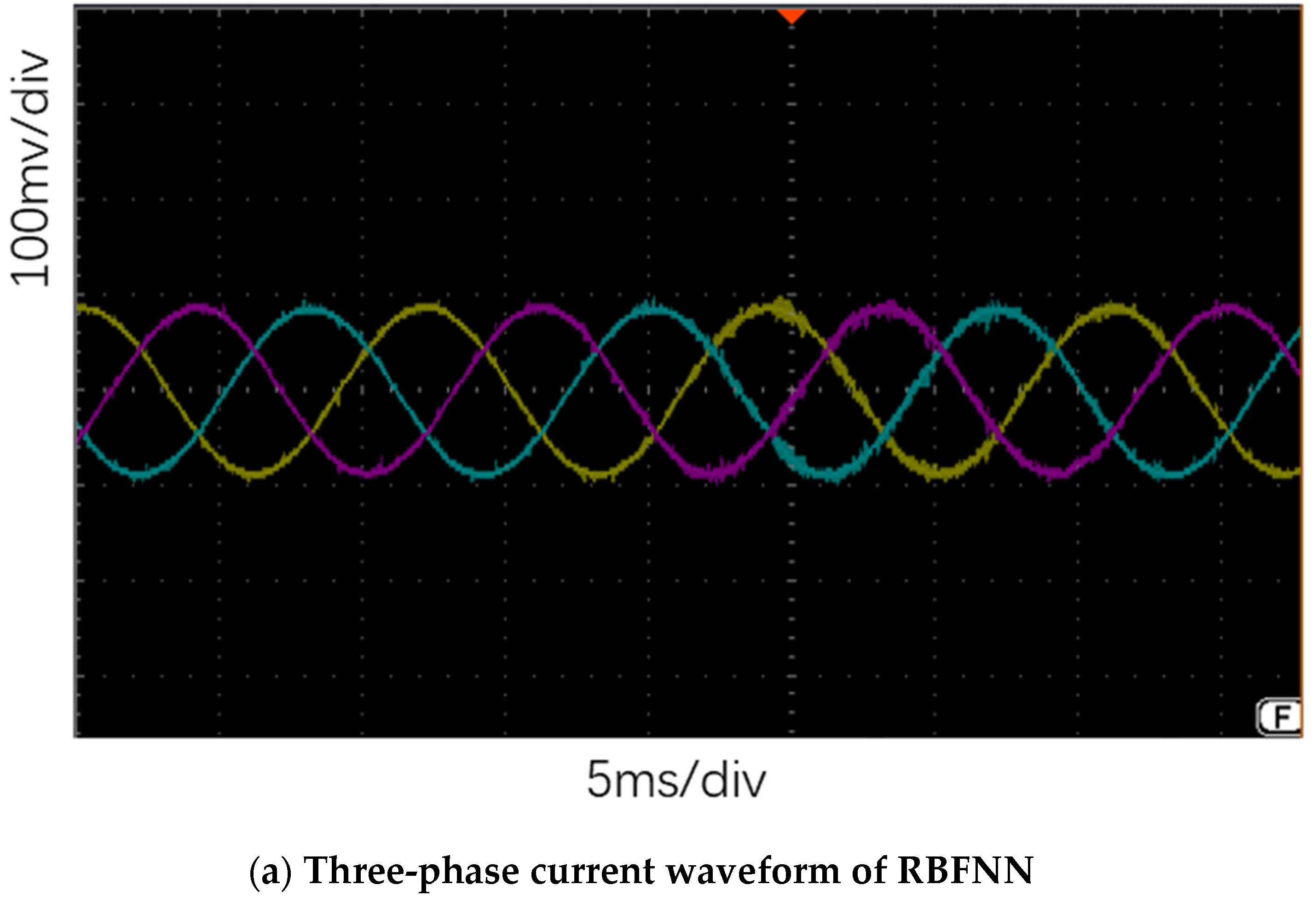
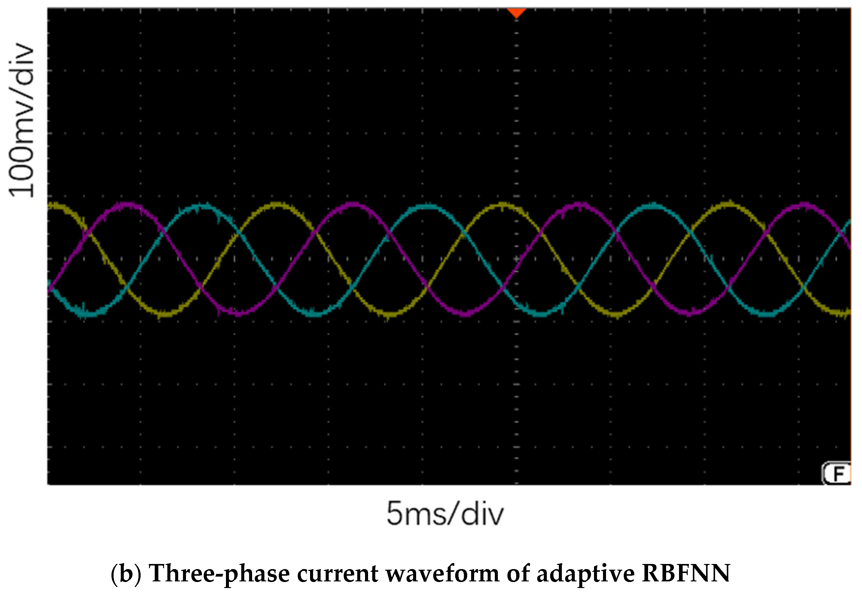
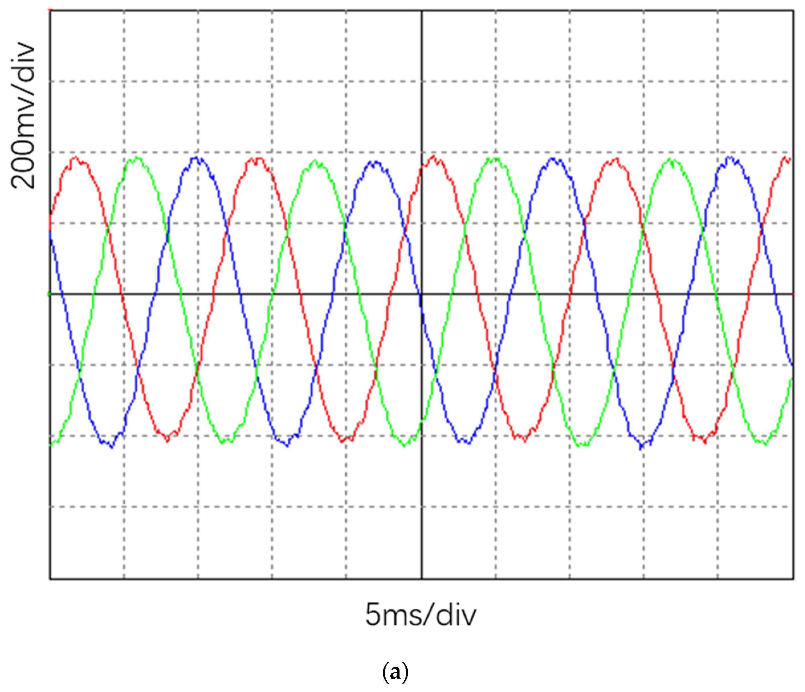
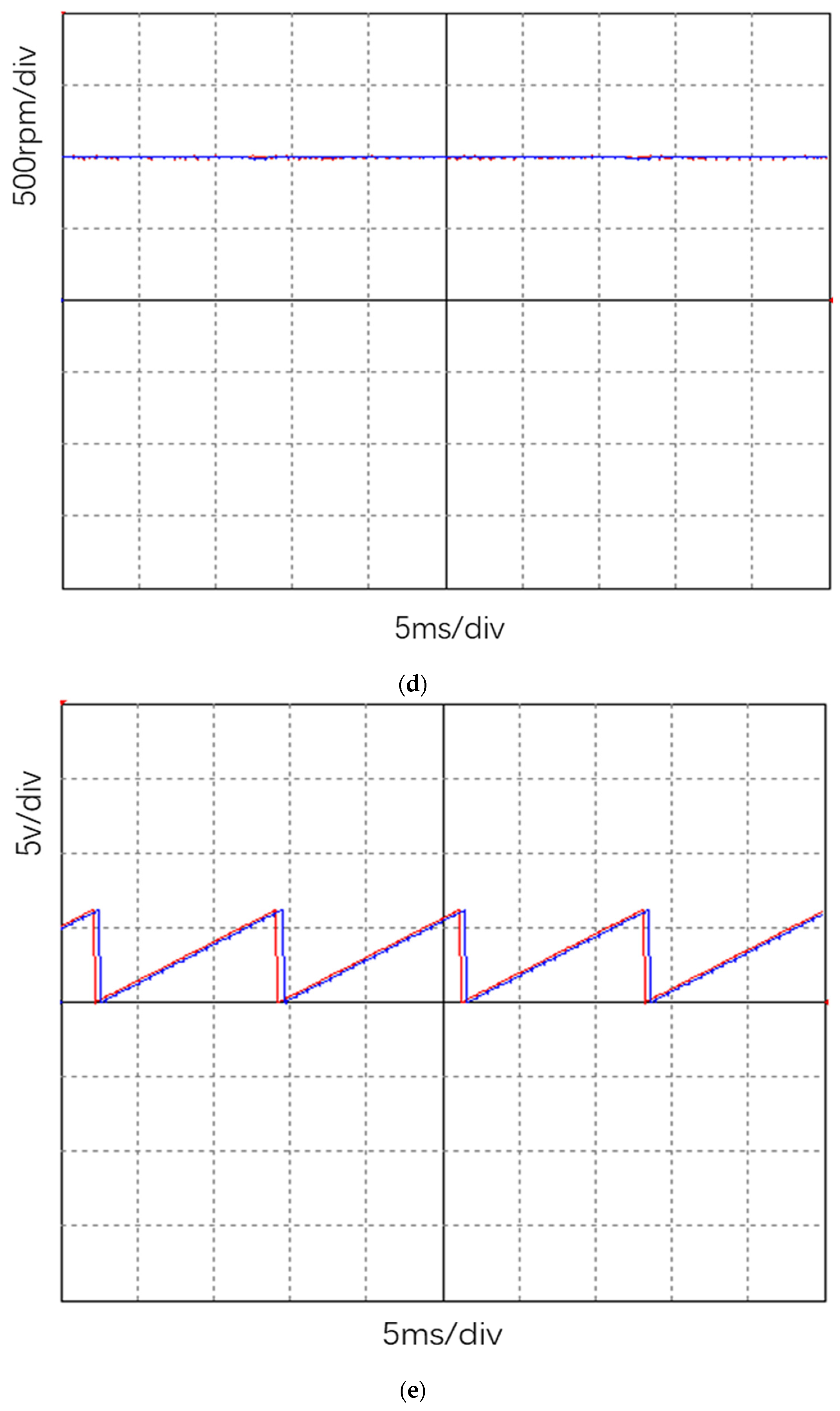
6.2. Experiment Results

By analyzing the mathematical model of SPMSM, the sensorless control method, and the design of the hardware system, the experiment platform can be set up. The core of the platform includes a power source, oscilloscope, drive circuit, and ac servo motor. TMS320F28335 is used as the core of the control system, before powering the ac servo motor, the first step is to determine whether the driving signal applied to the switching device meets the requirements. This driving signal can make the servo motor operate normally by controlling the switching tube of the inverter in the driving circuit. Only when the output driving signal meets the standard conditions can the motor be powered, otherwise the motor may be burned. After confirming that the main control chip can output the control signal, the sensorless control experiment of the ac servo motor is carried out. The experiment was carried out when the rotational speed reached 1000 rpm, and the operation of the position-free control system under sliding mode control was realized. The specific parameter of the servo motor in this experiment can be seen in

Table 2. Specific parameter of ac servo motor.

Rated Voltage	48 V
Rated Speed	1000 RPM
Rated Power	1 kW
Rated Torque	3.18 N
Stator Resistance	0.2 Ω
Pole	6 poles

. The waveform of the three-phase stator current is shown in the Figure 13.

Figure 13 shows the comparison of the three-phase current waveform before and after using the adaptive algorithm in RBFNN, as can be seen, under same circumstance, the harmonic wave is eliminated obviously. Figure 14 shows the waveform gathered by upper computer software, (d) shows the proposed method can track reference value correctly, (e) shows the rotor position can be predicted precisely, and (f) shows the rotor speed can transit to a higher value rapidly nearly without any overshoot.

7. Conclusions

This paper mainly focuses on optimizing the adaptive terminal sliding mode control using a radial neural network. Firstly, the modeling of SPMSM has been established and investigated, and the stability of the model is also verified. PSIM is a powerful software for electronic demonstration and motor drive simulation. The PSIM simulation results provide a theoretical foundation, and the algorithm is designed based on the simulation model. The PSIM experiment result can end convergence in a limited time with the given strategy. In the end, GaN, the advanced material, is used for a three-phase inverter in building hardware.

References

1. Xiao, S.; Shi, T.; Li, X.; Wang, Z.; Xia, C. Single-Current-Sensor Control for PMSM Driven by Quasi-Z-Source Inverter. IEEE Trans. Power Electron. 2019, 34, 7013–7024. [Google Scholar] [CrossRef]
2. Wang, W.; Yan, H.; Xu, Y.; Zou, J.; Zhang, X.; Zhao, W.; Buticchi, G.; Gerada, C. New Three-Phase Current Reconstruction for PMSM Drive with Hybrid Space Vector Pulsewidth Modulation Technique. IEEE Trans. Power Electron. 2021, 36, 662–673. [Google Scholar] [CrossRef]
3. Tang, Q.; Shen, A.; Li, W.; Luo, P.; Chen, M.; He, X. Multiple-Positions-Coupled Sampling Method for PMSM Three-Phase Current Reconstruction With a Single Current Sensor. IEEE Trans. Power Electron. 2020, 35, 699–708. [Google Scholar] [CrossRef]
4. Wang, W.; Yan, H.; Xu, Y.; Zou, J.; Buticchi, G. Improved Three-Phase Current Reconstruction Technique for PMSM Drive with Current Prediction. IEEE Trans. Ind. Electron. 2022, 69, 3449–3459. [Google Scholar] [CrossRef]
5. Jin, S.; Gu, J.; Jin, W.; Zhang, Z.; Zhang, F. Sensorless Control of Low Speed PMSM Based on Novel Sliding Mode Observer. In Proceedings of the 2021 IEEE 4th International Electrical and Energy Conference (CIEEC), Wuhan, China, 17 August 2021; pp. 1–5. [Google Scholar] [CrossRef]
6. Ilioudis, V.C.; Margaris, N.I. Sensorless Sliding Mode Observer based on rotor position error for salient-pole PMSM. In Proceedings of the 2009 17th Mediterranean Conference on Control and Automation, Thessaloniki, Greece, 24–26 June 2009; pp. 1517–1522. [Google Scholar] [CrossRef]
7. Zhou, Q.; Zhang, Y.; He, H.; Li, W.; Qi, X. Study on Location Detection of PMSM Rotor Based on Sliding Mode Observer. In Proceedings of the 2016 International Symposium on Computer, Consumer and Control (IS3C), Xi’an, China, 4–6 July 2016; pp. 77–80. [Google Scholar] [CrossRef]
8. Yang, C.; Ma, T.; Che, Z.; Zhou, L. An Adaptive-Gain Sliding Mode Observer for Sensorless Control of Permanent Magnet Linear Synchronous Motors. IEEE Access 2018, 6, 3469–3478. [Google Scholar] [CrossRef]
9. Liang, D.; Li, J.; Qu, R.; Kong, W. Adaptive Second-Order Sliding-Mode Observer for PMSM Sensorless Control Considering VSI Nonlinearity. IEEE Trans. Power Electron. 2018, 33, 8994–9004. [Google Scholar] [CrossRef]
10. Qiao, Z.; Shi, T.; Wang, Y.; Yan, Y.; Xia, C.; He, X. New Sliding-Mode Observer for Position Sensorless Control of Permanent-Magnet Synchronous Motor. IEEE Trans. Ind. Electron. 2013, 60, 710–719. [Google Scholar] [CrossRef]
11. Ye, S.; Yao, X. An Enhanced SMO-Based Permanent-Magnet Synchronous Machine Sensorless Drive Scheme With Current Measurement Error Compensation. IEEE J. Emerg. Sel. Top. Power Electron. 2021, 9, 4407–4419. [Google Scholar] [CrossRef]
12. Kivanc, O.C.; Ozturk, S.B. Sensorless PMSM Drive Based on Stator Feedforward Volt-age Estimation Improved With MRAS Multiparameter Estimation. IEEE/ASME Trans. Mechatron. 2018, 23, 1326–1337. [Google Scholar] [CrossRef]
13. Zhang, Z.; Liu, Y.; Liang, W.; Peng, J. MRAS Sensorless Control Strategy of PMSM based on SiC-MOSFET Three-Phase Inverter. In Proceedings of the 2020 IEEE 9th International Power Electronics and Motion Control Conference (IPEMC2020-ECCE Asia), Nanjing, China, 29 November–2 December 2020; pp. 1488–1492. [Google Scholar] [CrossRef]
14. Ouyang, Y.; Dou, Y. Speed Sensorless Control of PMSM Based on MRAS Parameter Identification. In Proceedings of the 2018 21st International Conference on Electrical Machines and Systems (ICEMS), Jeju, Korea, 7–10 October 2018; pp. 1618–1622. [Google Scholar] [CrossRef]
15. Ni, Y.; Shao, D. Research of Improved MRAS Based Sensorless Control of Permanent Magnet Synchronous Motor Considering Parameter Sensitivity. In Proceedings of the 2021 IEEE 4th Advanced Information Management, Communicates, Electronic and Automation Control Conference (IMCEC), Chongqing, China, 18–20 June 2021; pp. 633–638. [Google Scholar] [CrossRef]
16. Badini, S.S.; Verma, V. A Novel MRAS Based Speed Sensorless Vector Controlled PMSM Drive. In Proceedings of the 2019 54th International Universities Power Engineering Conference (UPEC), Bucharest, Romania, 3–6 September 2019; pp. 1–6. [Google Scholar] [CrossRef]
17. Wang, Z.; Zheng, Y.; Zou, Z.; Cheng, M. Position Sensorless Control of Interleav-ed CSI Fed PMSM Drive with Extended Kalman Filter. IEEE Trans. Magn. 2012, 48, 3688–3691. [Google Scholar] [CrossRef]
18. Zwerger, T.; Mercorelli, P. Combining SMC and MTPA Using an EKF to Estimate Parameters and States of an Interior PMSM. In Proceedings of the 2019 20th International Carpathian Control Conference (ICCC), Krakow-Wieliczka, Poland, 26–29 May 2019; pp. 1–6. [Google Scholar] [CrossRef]
19. Yang, H.; Yang, R.; Hu, W.; Huang, Z. FPGA-Based Sensorless Speed Control of PMSM Using Enhanced Performance Controller Based on the Reduced-Order EKF. IEEE J. Emerg. Sel. Top. Power Electron. 2021, 9, 289–301. [Google Scholar] [CrossRef]
20. Tondpoor, K.; Saghaiannezhad, S.M.; Rashidi, A. Sensorless Control of PMSM Using Simplified Model Based on Extended Kalman Filter. In Proceedings of the 2020 11th Power Electronics, Drive Systems, and Technologies Conference (PEDSTC), Tehran, Iran, 4–6 February 2020; pp. 1–5. [Google Scholar] [CrossRef]
21. Dai, Y.; Ye, C.; Zhao, S.; Yu, D.; Dian, R. EKF for Three-Vector Model Predictive Current Control of PMSM. In Proceedings of the 2020 IEEE 1st China International Youth Conference on Electrical Engineering (CIYCEE), Wuhan, China, 1–4 November 2020; pp. 1–6. [Google Scholar] [CrossRef]
22. Li, W.; Wen, X.; Zhang, J. Comparison of MRAS and SMO method for sensorless PMSM drives. In Proceedings of the 2019 22nd International Conference on Electrical Machines and Systems (ICEMS), Harbin, China, 11–14 August 2019; pp. 1–4. [Google Scholar] [CrossRef]
23. Li, X.; Kennel, R. General Formulation of Kalman-Filter-Based Online Parame-ter Identification Methods for VSI-Fed PMSM. IEEE Trans. Ind. Electron. 2021, 68, 2856–2864. [Google Scholar] [CrossRef]
24. Smidl, V.; Peroutka, Z. Advantages of Square-Root Extended Kalman Filter for Sensorless Control of AC Drives. IEEE Trans. Ind. Electron. 2012, 59, 4189–4196. [Google Scholar] [CrossRef]
25. Zhou, C.; Zhou, Z.; Tang, W.; Yu, Z.; Sun, X. Improved Sliding-Mode Observer for Posi-tion Sensorless Control of PMSM. In Proceedings of the 2018 Chinese Automation Congress (CAC), Xi’an, China, 30 November–2 December 2018; pp. 2374–2378. [Google Scholar] [CrossRef]
26. Gao, T.; Zhou, Y.; Huang, J.; Wang, W.; Chen, G. A sliding-mode observer design for the unknown disturbance estimation of a PMSM. In Proceedings of the 27th Chinese Control and Decision Conference (2015 CCDC), Qingdao, China, 23–25 May 2015; pp. 5851–5855. [Google Scholar] [CrossRef]
27. Ilioudis, V.C.; Margaris, N.I. PMSM sensorless speed estimation based on sliding mode observers. In Proceedings of the 2008 IEEE Power Electronics Specialists Conference, Rhodes, Greece, 15–19 June 2008; pp. 2838–2843. [Google Scholar] [CrossRef]
28. Okte, M. Sathans Sliding-mode observer for estimating position and speed and mini-mizing ripples in rotor parameters of PMSM. In Proceedings of the 2018 2nd International Conference on Inventive Systems and Control (ICISC), Coimbatore, India, 19–20 January 2018; pp. 506–511. [Google Scholar] [CrossRef]
29. Ilioudis, V.C.; Margaris, N.I. Sensorless speed and position estimation of PMSM using sliding mode observers in γ-δ reference frame. In Proceedings of the 2008 16th Mediterranean Conference on Control and Automation, Ajaccio, France, 25–27 June 2008; pp. 641–646. [Google Scholar] [CrossRef]
30. Qi, L.; Jia, T.; Shi, H. A novel sliding mode observer for PMSM sensorless vector control. In Proceedings of the 2011 IEEE International Conference on Mechatronics and Automation, Beijing, China, 7–10 August 2011; pp. 1646–1650. [Google Scholar] [CrossRef]
31. Zhang, X.; Li, Z. Sliding-Mode Observer-Based Mechanical Parameter Estimation for Permanent Magnet Synchronous Motor. IEEE Trans. Power Electron. 2016, 31, 5732–5745. [Google Scholar] [CrossRef]
32. Longfei, J.; Yuping, H.; Jigui, Z.; Jing, C.; Yunfei, T.; Pengfei, L. Fuzzy Sliding Mode Control of Permanent Magnet Synchronous Motor Based on the Integral Sliding Mode Surface. In Proceedings of the 2019 22nd International Conference on Electrical Machines and Systems (ICEMS), Harbin, China, 11–14 August 2019; pp. 1–6. [Google Scholar] [CrossRef]
33. Li, W.; Du, Z.; Wang, W.; Wu, W. Composite Fractional Order Sliding Mode Control of Permanent Magnet Synchronous Motor Based on Disturbance Observer. In Proceedings of the 2019 Chinese Automation Congress (CAC), Hangzhou, China, 22–24 November 2019; pp. 4012–4016. [Google Scholar] [CrossRef]
34. Xu, C.; Wang, K.; Yang, X.; Zhang, B. Terminal Sliding Mode Control of Permanent Magnet Synchronous Motor Based on a Novel Adaptive Reaching Law. In Proceedings of the 2021 IEEE 4th Advanced Information Management, Communicates, Electronic and Automation Control Conference (IMCEC), Chongqing, China, 18–20 June 2021; pp. 1731–1735. [Google Scholar] [CrossRef]
35. Hou, H.; Yu, X.; Xu, L.; Rsetam, K.; Cao, Z. Finite-Time Continuous Terminal Sliding Mode Control of Servo Motor Systems. IEEE Trans. Ind. Electron. 2020, 67, 5647–5656. [Google Scholar] [CrossRef]
36. Junejo, A.K.; Xu, W.; Mu, C.; Ismail, M.M.; Liu, Y. Adaptive Speed Control of PMSM Drive System Based a New Sliding-Mode Reaching Law. IEEE Trans. Power Electron. 2020, 35, 12110–12121. [Google Scholar] [CrossRef]
37. El-Sousy, F.F.M.; Amin, M.; Mohammed, O.A. High-Precision Adaptive Back-stepping Optimal Control using RBFN for PMSM-Driven Linear Motion Stage. In Proceedings of the 2019 IEEE International Electric Machines & Drives Conference (IEMDC), San Diego, CA, USA, 12–15 May 2019; pp. 1680–1687. [Google Scholar] [CrossRef]
38. Jiao, L.; Zhang, P.; Min, R.; Luo, Y.; Yang, D. Research on PMSM Sensorless Control Based on Improved RBF Neural Network Algorithm. In Proceedings of the 2018 37th Chinese Control Conference (CCC), Wuhan, China, 25–27 July 2018; pp. 2933–2938. [Google Scholar] [CrossRef]
Figure 1. Common coordinates of SPMSM.
Electronics 11 01646 g001
Figure 2. The current and voltage limit circle of SPMSM under d-q axis.
Electronics 11 01646 g002
Figure 3. Different regions and vector composing: (a) voltage space vectors diagram in different regions. (b) reference voltage vector in a sector boundary region, V r e f 1 is reconstructable vector in reconstructable region, V r e f 2 is reconstructable vector in sector boundary region.
Electronics 11 01646 g003
Figure 4. Voltage reference vector in different regions and the output current.
Electronics 11 01646 g004
Figure 5. The current path of nonzero voltage reference vectors. (a) S a = 1 , S b = 0 and S c = 0 ; (b) S a = 1 , S b = 1 and S c = 0 ; (c) S a = 0 , S b = 1 and S c = 0 ; (d) S a = 0 , S b = 1 and S c = 1 ; (e) S a = 1 , S b = 1 and S c = 0 ; (f) S a = 0 , S b = 1 and S c = 0 .
Electronics 11 01646 g005
Figure 6. The current path of two zero voltage reference vectors. (a) S a = 1 , S b = 1 and S c = 1 ; (b) S a = 0 , S b = 0 and S c = 0 .
Electronics 11 01646 g006
Figure 7. The proposed schematic diagram of adaptive sliding mode control using radial basis function neural network.
Electronics 11 01646 g007
Figure 8. Block diagram of the overall hardware control system.
Electronics 11 01646 g008
Figure 9. Configuration of experimental setup.
Electronics 11 01646 g009
Figure 10. Simulation result of conventional SMC.
Electronics 11 01646 g010aElectronics 11 01646 g010b
Figure 11. Simulation result of RBFNN-SMC.
Electronics 11 01646 g011aElectronics 11 01646 g011b
Figure 12. Simulation result of adaptive RBFNN-SMC.
Electronics 11 01646 g012aElectronics 11 01646 g012b
Figure 13. Three-phase stator current waveform using conventional RBFNN and adaptive RBFNN.
Electronics 11 01646 g013aElectronics 11 01646 g013b
Figure 14. Waveform detected by human–machine interface. (a) Three-phase stator current waveform; (b) Clark transformed current; (c) SVPWM output waveform; (d) waveform diagram of actual speed and reference speed; (e) actual and estimated position of the rotor; (f) dynamic performance when changing the reference speed.
Electronics 11 01646 g014aElectronics 11 01646 g014bElectronics 11 01646 g014cElectronics 11 01646 g014d