
A Study on the Optimal Control of Voltage Utilization for Improving the Efficiency of PMSM


Electric Motor Control Laboratory, Graduate School of Automotive Engineering, Kookmin University, Seoul 02707, Korea
*
Author to whom correspondence should be addressed.
Electronics 2022, 11(13), 2095; https://doi.org/10.3390/electronics11132095
Submission received: 12 May 2022
/
Revised: 20 June 2022
/
Accepted: 22 June 2022
/
Published: 4 July 2022
(This article belongs to the Special Issue Advancements in Electric Motors, Drives, Power Converters and Related Systems)
Abstract
:When performing weak flux control to drive a permanent-magnet synchronous motor at high speed, the efficiency is lowered because the copper loss increases as the negative D-axis current increases. In addition, if the overmodulation index is slightly lowered and driven without setting it to the maximum value, the phase current ripple reduction effect can be expected compared to the six-step control. Therefore, if the motor is operated at a current point that can minimize the sum of copper loss and iron loss, the motor can be driven with maximum efficiency. In addition, if the overmodulation index is slightly lower than that of the six-step control, the phase current ripple can be reduced. This paper proposes a method for finding an overmodulation index to maximize driving efficiency when driving a motor based on the magnetic flux–torque command. In addition, an algorithm for driving a motor with maximum efficiency by applying an optimal overmodulation index table is proposed. Based on the MATLAB Simulink simulation, the efficiency change characteristics according to the overmodulation index change are reviewed, and the efficiency improvement and current ripple reduction effects are verified through a dynamometer experiment.
1. Introduction
As energy depletion and environmental problems arise, internal combustion engine devices using conventional fossil fuels are gradually being replaced with electric motors and battery systems. Accordingly, the need for research on algorithms for driving motors with a higher efficiency is being emphasized [1]. The efficiency of electric motors is directly related to environmental issues. In this paper, a method to improve the driving efficiency of permanent-magnet synchronous motors (PMSMs), which are most widely used for driving electric vehicles, is studied under high-speed operation.
In order to control the PMSM at a speed higher than the base RPM, it is necessary to perform flux-weakening control to reduce the air gap flux and thereby obtain a voltage margin [2,3]. In this situation, as the negative D-axis current increases very significantly, the magnitude of the phase current increases, meaning that the power loss due to copper loss increases [4,5]. If voltage utilization is increased through voltage overmodulation, the voltage margin can be obtained without increasing the phase current magnitude [6,7]. However, in this case, the phase current is distorted by harmonic components and power loss due to iron loss increases. Therefore, if the flux-weakening control and overmodulation control are properly performed, the power loss due to copper loss and iron loss can be minimized and the operating efficiency of the motor can be improved in the high-speed region.
Classically, the control method that minimizes the size of copper loss by selecting the current operating point at the boundary of the voltage-limiting ellipse has mainly been used [8,9]. However, since this control method does not consider iron loss, the driving efficiency of the motor is low. In other previous studies, control algorithms that consider iron loss and copper loss together to improve motor driving efficiency were proposed [10,11,12,13,14,15,16], but these are difficult to use in the region where the phase voltage is overmodulated. LMC (loss model control) is a method for calculating a current operating point using a mathematical model function of the current magnitude and driving frequency in order to minimize power loss. In this method, it is difficult to define a mathematical model for the change in power loss due to phase current ripples caused by voltage overmodulation [10,11,12,13,14,15,16]. In addition, the LMC method has the disadvantage that inaccurate parameter information leads to inaccurate calculation results of the current operating point for minimizing power loss. On the other hand, the SC (search control) algorithm measures the input power in real time and adjusts the phase angle of the current so that the magnitude of the input power is minimized [14]. In this method, there is a very high possibility that the control will diverge and become unstable in the overmodulation control region where the voltage margin is insufficient.
Therefore, in this paper, we propose a control method that reflects the copper loss and iron loss of the motor, which were not considered in the existing overmodulation control. We then create an overmodulation index table in the form of a 3D lookup table. The most efficient overmodulation index for each torque operating point is stored in this table. Using this overmodulation index table, the current operating point at which the maximum efficiency is output is determined through the magnetic flux–torque current map. The proposed method was verified through MATLAB Simulink. In addition, the algorithm was validated by dynamometer testing.
2. Current Operating Point for Motor Loss Reduction Control
Figure 1 shows the change in copper loss and iron loss according to the movement of the current operating point in the D–Q axis current plane of the IPMSM motor. The magnitude of copper loss is proportional to the square of the current magnitude, and it can be expressed using Equation (1) [13].
The magnitude of the iron loss is very non-linear, so it is difficult to accurately express it with an equation. However, since it is known that the magnitude increases in proportion to the motor driving frequency and the magnitude of the magnetic flux, it can be expressed in a simplified manner in Equation (2) [4].
2.1. The Tendency of Power Loss to Change Due to the Movement of the Current Operating Point
In order to maintain the output torque of the motor regardless of speed or voltage change, the current operating point must move along a constant torque curve. If the current operating point moves to the left on the constant torque curve, the copper loss increases because the current operating point moves away from the origin. At the same time, the iron loss decreases because the magnitude of the air gap flux decreases. On the other hand, if the current operating point moves to the right, the magnitude of the current decreases as the distance from the origin increases, and the copper loss decreases. At the same time, the size of the iron loss increases. As described above, changes in copper loss and iron loss according to the movement of the current operating point are in an inverse proportion to each other. Therefore, if the current operating point is appropriately selected to minimize the total loss, including the iron loss and the copper loss, the efficiency of the motor can be increased.
2.2. Current Operating Point Selection Strategy in the D–Q Axis Current Plane
Figure 2 shows a comparison between the algorithm proposed in this study and the algorithms proposed in previous studies with respect to the strategy used for selecting the D–Q axis current operating point. The selectable area of the current operating point is limited inside the voltage-limiting ellipse and the current-limiting circle [17]. If the speed of the motor is and the battery voltage is given as , the voltage-limiting ellipse is given as ‘B’ when the overmodulation control is performed to the minimum. In the classical control considering only copper loss, the current magnitude is minimized by selecting the ‘b’ point, which is the intersection of the voltage-limiting ellipse and the constant torque curve. The LMC and SC methods considering both iron loss and copper loss select the current operating point ‘a’. In this case, compared to point ‘b’, the copper loss slightly increases as the current increases, but the efficiency is improved because the iron loss decreases as the air gap flux decreases.
If voltage utilization is maximized through voltage overmodulation, the selectable current range expands as the voltage-limiting ellipse ‘A’. In previous studies, copper loss and iron loss were not considered together in the voltage overmodulation control region (intermediate region between the ‘A’ and ‘B’ ellipses). In order to minimize copper loss, a six-step control that always maintains the maximum voltage utilization rate was performed, or overmodulation control was temporarily performed to improve control stability when the voltage was temporarily insufficient. Six-step control is a control method that selects the ‘d’ point, which is the intersection of the voltage-limiting ellipse and the constant torque curve, and drives the motor with the smallest current magnitude. In the case of the algorithm proposed in this study, point ‘c’ is selected, and the maximum efficiency can be achieved because the motor operates at the current operating point where copper and iron losses are minimized in the overmodulation control region.
On the other hand, if the motor has to operate on the MFPT (Minimum Flux per Torque: MFPT) curve because the speed of the motor is very high, as for or when the battery voltage is low, the output torque is maximized only when the overmodulation control is performed to the maximum. If the overmodulation control is not performed, the maximum output cannot be produced by operating at the operating point ‘e’. Therefore, in this case, the output torque and efficiency can be maximized only by driving at the current operating point ‘f’ [18].
3. Voltage Overmodulation
The algorithm proposed in this study improves the driving efficiency of the motor by moving the current operating point to the extended current operating region by voltage overmodulation. Voltage overmodulation increases the size of the voltage-limiting ellipse, which means that the range of selectable current operating points is widened. Then, the current operating point can be selected from the wide area in order to increase the driving efficiency [19,20,21,22].
3.1. Implementation of Bolognani Voltage Overmodulation
Figure 3 shows the voltage modulation method proposed by Bolognani in the polar coordinate system [23]. The magnitude of the resultant vector , which is the sum of the three-phase voltage vectors , , and , is limited inside the voltage hexagon.
The maximum magnitude of the voltage that can be freely generated regardless of the voltage phase is , and the voltage output can be increased up to this voltage level without generating harmonics in the current. However, it is impossible to generate a voltage higher than because it may exceed the voltage hexagon depending on the phase. As shown in Figure 3, if the voltage command cannot be generated because it is outside the hexagon, of the same magnitude can be generated by selecting a new phase, . The equation to implement this is given as follows.
The maximum output voltage that can be achieved through overmodulation control is and the maximum effective applied voltage of the fundamental frequency is . In this study, the voltage overmodulation index (MI) is defined as follows for easy analysis:
when voltage overmodulation is performed to the minimum, the overmodulation index is , and when voltage overmodulation is performed to the maximum, the overmodulation index of the effective voltage is .
3.2. Nonlinearity Compensation of Overmodulated Voltage
Figure 4 shows the comparison of the magnitudes of the fundamental frequency components included in the command voltage and the output voltage when Bolognani voltage overmodulation is performed. Since the voltage command exceeding MI = 1.1547 includes harmonics, the fundamental frequency component of the output voltage effectively applied to the motor becomes smaller than the command voltage.
Therefore, in order to apply a desired voltage to the motor, the voltage command must be compensated, as shown in Figure 5.
4. Optimal Voltage Utilization Control Algorithm
4.1. Block Diagram of Voltage Utilization Optimal Control Algorithm
Figure 6 is a block diagram of the algorithm proposed in this paper to control the motor with maximum efficiency. In the classical algorithm, the current references are determined based on the torque command and the magnetic flux command is calculated by dividing the voltage by the speed.
However, the proposed algorithm determines the current references based on , which is an actively controlled magnetic flux reference, instead of . The proposed algorithm is a control algorithm that moves the current operating point so that power loss due to copper and iron loss is minimized by adjusting the magnetic flux command through MI PI control. In order to implement this algorithm, the ‘Optimal MI Table’ must be created by measuring the optimal MI for each speed and voltage condition through a dynamometer experiment.
The D–Q axis current commands and are determined from the 3D current map based on the magnetic flux command and the torque command . From 0 speed to the BASE RPM area, the operation at the MTPA driving point is the maximum efficiency driving point. If it exceeds the base rpm, the algorithm proposed in this paper is applied from the area where the weak magnetic flux begins. If is properly adjusted, the current operating point can be shifted in the direction of decreasing or increasing magnetic flux on a constant torque curve. If the current command is shifted in the direction of increasing the magnetic flux, the back EMF generated in the motor coil increases and the output voltage required for current control increases. In this situation, the current control algorithm actively performs overmodulation control to increase the voltage utilization rate. Conversely, if the current command is shifted in the direction of decreasing the magnetic flux, the magnitude of the voltage required for current control becomes smaller and the current control algorithm lowers the voltage utilization rate. As a result, by adjusting the magnetic flux command input to the current map, it is possible to control the output voltage utilization rate of the inverter.
By applying the principle described above, the current operating point can be moved so that the driving efficiency of the motor is maximized. Moreover, if the optimal is already known through the experiment, the magnetic flux command can be adjusted to the optimal value by performing the ‘MI PI control’ and, as a result, the motor can be operated at the current operating point showing the highest efficiency.
determined as a result of ‘MI PI control’ is added to the existing magnetic flux command to adjust to an optimal value. In other words, maintains the inverter’s voltage utilization at an optimal value in real time, leading the motor to operate at maximum efficiency.
On the other hand, if the magnetic flux–torque current map is inaccurate to some degree, the magnetic flux command can be corrected by applying the ‘magnetic flux command correction table’. is the magnetic flux reference value that is experimentally measured so that the magnitude of the phase reference voltage becomes . This table is not necessary if the flux–torque current map is very accurate.
4.2. Strategies for Obtaining an Optimal MI According to Speed Range
Figure 7 shows the optimal-MI acquisition strategy proposed in this study, dividing it into three stages. Part A is a low-speed region where there is no need for flux-weakening control or overmodulation control because the voltage margin is sufficient. Part B is a medium-speed region that operates on a constant torque curve and performs flux-weakening control or overmodulation control to obtain a voltage margin. Part C is a high-speed region where the speed can be increased only by lowering the magnitude of the output torque.
- Part A: MTPA (Maximum Torque per Ampere: MTPA) operation region
At a low speed below the base RPM, where the voltage margin is sufficient, flux-weakening control or overmodulation control is not necessary. The motor is driven at the MTPA current operating point, keeping the voltage modulation index below 1.1547.
- 2.
- Part B: Constant torque curve operating region
In this speed region, flux-weakening control or overmodulation control must be performed to obtain a voltage margin. The control algorithm adjusts the overmodulation index to an optimal value in the range of 1.1547 to 1.2732 so that the driving efficiency of the motor is maximized.
- 3.
- Part C: MFPT curve operating region
This is a high-speed region where the motor can be driven only by reducing the output torque. In this region, as the overmodulation index increases, the output torque and output power increase. In order to maximize the performance and efficiency of the motor, it is always operated by controlling the overmodulation index to the maximum of 1.2732.
5. Simulation in MATLAB Simulink (MATLAB 2017b Academic Ver.)
The RT model of the 100 kW IPMSM motor was applied and a simulation was performed with MATLAB Simulink. While changing MI from 1.1547 to 1.2732, changes in the power loss and motor efficiency were reviewed.
5.1. Simulation Configuration
Figure 8 shows the simulink block used in the simulation. The motor model applied to the simulation is a 100 kW IPMSM model provided as an example by JMAG. This RT model is generated based on the electric/mechanical shape information of the motor, and when a three-phase input voltage is applied, the output torque and phase current waveforms are output very similarly to the actual ones. In addition, since the iron loss and copper loss of the motor can be checked in real time, it is easy to monitor which loss component changes the efficiency of the motor.
5.2. Efficiency Change According to MI Change
5.2.1. Efficiency Change According to MI Change on Constant Torque Curve
Figure 9 shows the trajectory of the current operating point when the voltage overmodulation index is changed under the conditions of a 5000 RPM speed and a 250 V voltage. During the simulation, a constant load torque was applied and the speed was controlled to a constant value; the output power thus remained almost constant. Since the same output torque was generated, the current operating point moved along a constant torque curve. The voltage overmodulation index was controlled in 41 steps from 1.1547 to 1.2732, and the efficiency was measured in the steady state. The results are shown in Figure 10.
As the voltage overmodulation index increased, copper loss decreased and iron loss increased. Since the output power was constant, the ratio of loss/output showed the same trend as the integrated loss. As the overmodulation index increased, the efficiency of the motor increased, but when the overmodulation index became too large, the efficiency decreased. The maximum efficiency was shown in the overmodulation index of about 1.24. The overmodulation index for the maximum efficiency of the motor may be different depending on the parameters determining the magnitude of the copper loss and iron loss of the motor.
In conclusion, when the current operating point is on a constant torque curve, the efficiency of the motor can be maximized by slightly lowering the overmodulation index from the maximum in order to reduce the iron loss.
5.2.2. Efficiency Change According to MI Change on MFPT Curve
Figure 9 shows the trajectory of the current operating point when the voltage overmodulation index is changed under the conditions of an 8500 RPM speed and a 170 V voltage. Since the current operating point is in the MFPT curve, it shows a different trend compared to the case of the constant torque curve. The results are shown in Figure 11.
Figure 12 shows the results for the MFPT curve. In the MFPT curve, as the overmodulation index increases, the current operating point moves away from the origin. Therefore, copper loss increases in proportion to the magnitude of the phase current. Furthermore, as the overmodulation index increases, the magnitude of the iron loss increases. This is because the magnitude of the harmonics included in the phase current increases, and the magnitude of the air gap magnetic flux also increases. Therefore, when the overmodulation index increases on the MFPT curve, both the copper loss and the iron loss increase, meaning that the total electrical loss increases. However, despite the increase in the loss component, the efficiency of the motor increases as the overmodulation index increases because the output power increases when the output torque increases.
In conclusion, if the current operating point moves on the MFPT curve, the overmodulation index should be controlled to the maximum value in order to maximize the efficiency of the motor. In addition, on the MFPT curve, the output torque of the motor can be used to the maximum only when the voltage modulation index is controlled to the maximum.
6. Experiment in Dynamometer
6.1. Dynamometer Experimental Equipment
A dynamometer device that could measure real-time efficiency while driving IPMSM with a three-phase inverter was configured. The input voltage and current were measured from the DC power supply, and the speed and torque information of the motor could be obtained from the torque sensor and the powder brake. Based on this information, the efficiency of the system was calculated in the power analyzer.
The torque loader was set to maintain a constant load torque and the three-phase inverter controlled the motor at a constant speed. In this way, the experimental equipment was configured to easily observe the change in efficiency according to the change in the overmodulation index under constant speed, torque, and voltage conditions. The configuration of the test environment is shown in Figure 13.
6.2. Experiment to Observe the Change in Efficiency According to the MI Change
Figure 14 shows the results of measuring the efficiency of the motor while changing the MI from 1.1547 to 1.2732 under the four test conditions. Since a constant load torque was applied, the current operating point moved along the constant torque curve.
Similar to the simulation results, at test points B and D close to the MTPA curve, the efficiency gradually increased as the MI increased in the region where the MI was small, and the efficiency began to decrease when the MI became very large. This was because when the voltage modulation index increased and the current operating point moved, the decrease in copper loss was insignificant but the increase in iron loss was large.
On the other hand, at test points A and C, which were far away from the MTPA curve, the efficiency continued to increase as the MI increased. This was because when the voltage modulation index increased and the current operating point moved, the copper loss decreased significantly while the iron loss increased only slightly. The difference in the magnitude of the current when the voltage modulation index was 1.1547 and when it was 1.2732 was large; thus, it seems that copper loss was greatly reduced.
As a result, depending on the current operating region, it may be necessary to control the MI to a maximum value or to a slightly smaller value in order to maximize the motor efficiency. In order to always control the efficiency of the motor to the maximum, it is necessary to find the optimal MI in the entire current operating area and apply it in a table.
6.3. Experimental Method for Creating an Optimal MI Table
As in the experiment performed in Section 6.2, if the efficiency is measured while changing the voltage modulation index from 1.1547 to 1.2732 under specific speed, voltage, and load torque conditions, it is possible to find out which MI shows the maximum efficiency. The optimal MI table can be created by setting test points in the entire area of the current map and finding the optimal MI for each test point to maximize efficiency.
Figure 15 shows the test points used for creating the optimal MI table. For each load torque and battery voltage condition, the current operating points when controlled with MI = 1.1547 are circled. In addition, the motor efficiency was measured while increasing the MI at each operating point, and the MI value that maximized the efficiency was written in the number above the circle.
Figure 16 shows the optimal MI value shown in Figure 15 by matching the magnetic flux and torque commands of the current map. MI values can be identified by color.
Figure 17 shows the optimal MI table with increased resolution from interpolating and extrapolating the data obtained from the test points. The ranges of the magnetic flux and torque commands expressed in the X and Y axes were set to be the same as the commands used in the current map. This was because it was easy to apply the optimal MI table to all regions of the current map.
If more test points are set by subdividing the load torque and DC voltage test conditions, more precise results can be obtained. However, since it is time-consuming to control the MI in many steps for each test point and measure the efficiency, it is more efficient to increase the resolution by measuring at a small number of test points and then interpolating and extrapolating them.
Figure 18 shows the optimal MI data with the same resolution as the current map expressed on the D–Q axis current plane. The circled points mean that the current operating points are to be selected if the MI is controlled to 1.1547. Moreover, if MI is controlled to the optimum value written on the circle, the current operating point will shift.
6.4. Optimal MI Table Application Experiment
By applying the optimal MI table, a real-time efficiency improvement verification test was conducted. Experiments were conducted at current operating points near the MTPA curve, where a marked improvement in efficiency was observed.
The left side of Figure 19 shows the current operating points when MI = 1.1547, MI = 1.2732, and MI = optimal table values are applied. When the MI was controlled to 1.1547 and 1.2732, a fixed MI command value was input to the MI feedback controller. When the optimum MI was controlled, the MI input was automatically determined from the optimum MI table according to the speed and voltage conditions.
Table 1 shows the results of the efficiency comparison experiment. When the optimal MI was applied, the maximum efficiency improvement was about 2% compared to the case where MI = 1.1547 was applied, and about 0.3% compared to the case where MI = 1.2732 was applied.
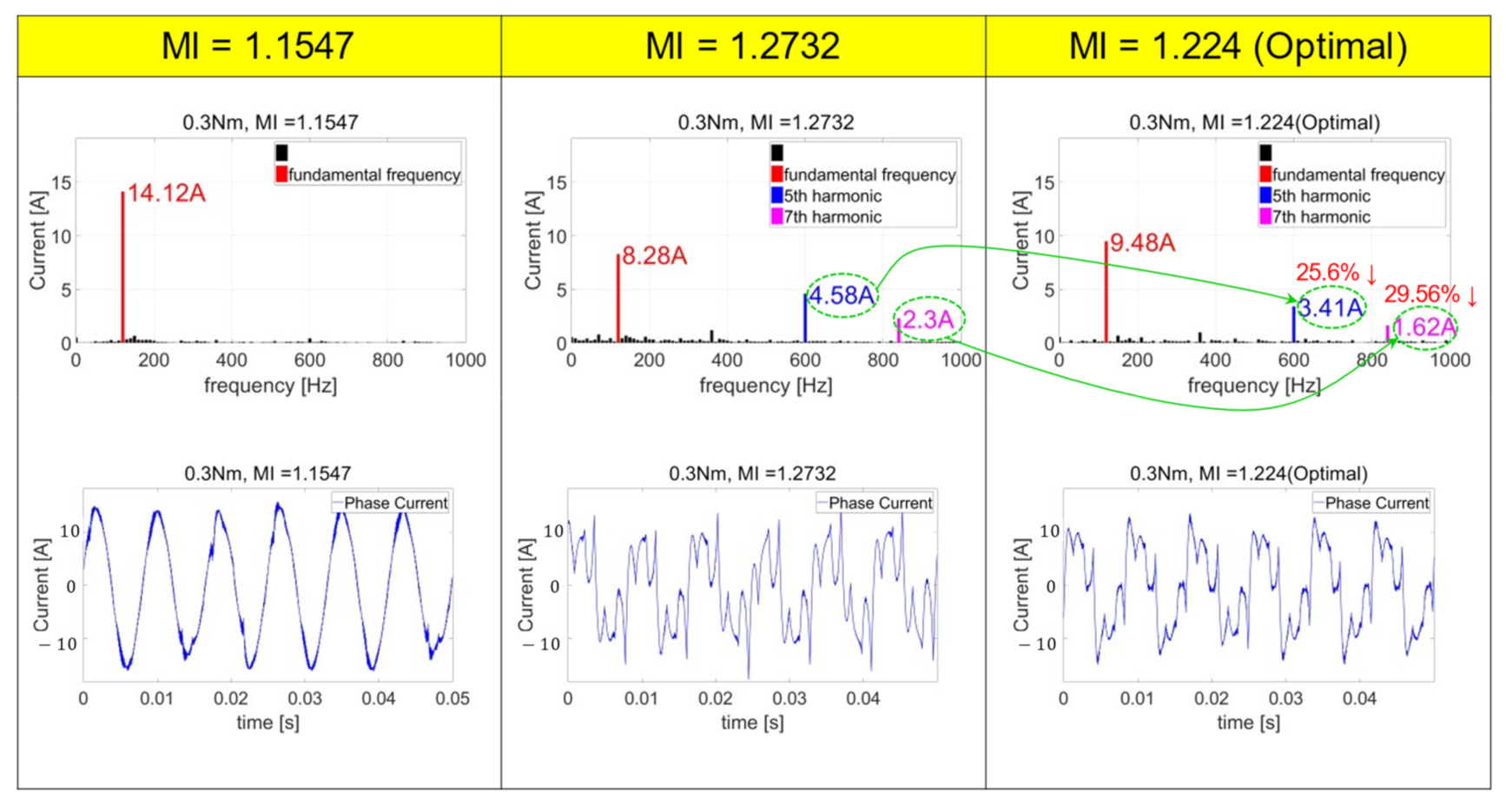
Figure 20 shows the phase current waveform and FFT analysis results obtained during the experiment in Section 6.4. The test conditions were 0.3 Nm, 1800 RPM, and 10.3 V [24].
When MI was controlled to 1.1547, the phase current was close to a sine wave. Even in the FFT analysis result, there was no noticeable ripple component and there was only a small amount of high-frequency noise.
On the other hand, in the case of MI = 1.2732, the phase current waveform was very distorted. According to the FFT analysis result, the magnitude of the current at the fundamental frequency was the smallest among the three, but the fifth and seventh harmonic components were very large. When MI was controlled to an optimal value, compared to the case where MI = 1.2732 was controlled, the magnitude of the current of the fundamental frequency slightly increased, but the fifth and seventh harmonic components were reduced by 25–30%. When the phase current ripple is reduced, the stability of the control can be improved during current feedback control, and this is advantageous in improving the torque ripple and noise of the motor. In conclusion, if the optimal MI table is used, the efficiency can be higher, and the phase current ripple can be reduced compared to when the MI is controlled to the maximum value.
7. Conclusions
In this paper, we proposed a method for finding the optimal voltage modulation index for driving a permanent-magnet synchronous motor with maximum efficiency and organizing it into a table. We also devised a real-time control algorithm that drives the motor while maintaining the voltage utilization of the inverter at an optimal value.
Through a MATLAB simulation, the characteristics of the efficiency change according to the change in the MI value were examined. An optimal MI table was created through actual dynamometer testing, and improved efficiency and current ripple reduction effects were verified. When the optimal MI was applied, it was confirmed that the efficiency was improved by up to 2% compared to the MI = 1.1547 control method and up to 0.3% compared to the MI = 1.2732 control method. In addition, it was confirmed that the magnitude of harmonic ripple currents could be reduced by up to 30% compared to the six-step control method. In this study, external environmental changes were not considered. For applications, further research is needed on the impact of the environment changing during motor driving. For example, the maximum efficiency operating point may be changed due to a change in the current operating point according to a change in motor parameters, such as a change in temperature. To cope with this case, further research is needed on the calibration method of the magnetic flux–torque current map and the optimal overmodulation MI table for each temperature. In addition, due to experimental environmental limitations, algorithm verification for 1 kW motors has been performed, but it can also be applied to high-power motors. Future research needs to verify how much efficiency can be improved when applied to high-power motors.
Author Contributions
Conceptualization, J.-H.P.; Methodology, J.-H.P.; Software, J.-H.P.; Validation, J.-H.P.; Formal analysis, J.-H.P.; Investigation, J.-H.P.; Resources, H.-S.L.; Data curation, H.-H.L.; writing—original draft preparation, J.-H.P.; writing—review and editing, J.-H.P.; Visualization, H.-S.L.; Supervision, G.-H.L.; Project administration, H.-H.L.; Funding acquisition, H.-H.L.; All authors have read and agreed to the published version of the manuscript.
Funding
This research was supported by Korea Institute for Advancement of Technology(KIAT) grant funded by the Korea Government(MOTIE)(P0017120, The Competency Development Program for Industry Specialist) and This Research was funded and conducted under Technology Innovation Program (NO.20011866, Hydrogen Truck Electrical and Power Parts Localization Technology Development Project) funded By the Ministry of Trade, Industry & Energy(MOTIE, Korea).
Institutional Review Board Statement
Not applicable.
Informed Consent Statement
Not applicable.
Data Availability Statement
Data sharing is not applicable to this article.
Conflicts of Interest
The authors declare no conflict of interest.
References
- Ning, Y.; Gong, Y.-M. High Dynamic Performance Speed Control Strategy of High Density IPMSM for HEV Application. In Proceedings of the 2008 7th World Congress on Intelligent Control and Automation, Chongqing, China, 25–27 June 2008; pp. 1588–1593. [Google Scholar]
- Lee, J.H. Field-weakening strategy in condition of DC-link voltage variation using on electric vehicle of IPMSM. In Proceedings of the 2011 International Conference on Electrical Machines and Systems, Beijing, China, 20–23 August 2011. [Google Scholar]
- Zhang, X.; Wang, B.; Yu, Y.; Zhang, J.; Xu, D. Overmodulation Index Optimization Method for Torque Quality Improvement in Induction Motor Field-Weakening Control. IEEE Trans. Ind. Electron. 2021, 68, 11954–11967. [Google Scholar] [CrossRef]
- Lee, J. Loss-Minimizing Control of PMSM With the Use of Polynomial Approximations. IEEE Trans. Power Electron. 2009, 24, 1071–1082. [Google Scholar]
- Shen, J.-X.; Qin, X.-F. Investigation of Rotor Eddy Current Loss in High-Speed PM Synchronous Motor with Various PWM Strategies. In Proceedings of the 2020 Fifteenth International Conference on Ecological Vehicles and Renewable Energies (EVER), Monte-Carlo, Monaco, 10–12 September 2020; pp. 1–5. [Google Scholar] [CrossRef]
- Kwon, T.-S.; Choi, G.Y.; Kwak, M.S.; Sul, S.K. Novel Flux-Weakening Control of an IPMSM for Quasi-Six-Step Operation. IEEE Trans. Ind. Appl. 2008, 44, 1722–1731. [Google Scholar] [CrossRef]
- Kwon, S.; Son, D.; Lim, H.; Park, J.; Baek, H.; Lee, G.-H. Overmodulation Strategy Using DC-Link Shunt Resistor Inverters to Maintain Output Voltage Linearity. IEEE Access 2021, 9, 160812–160822. [Google Scholar] [CrossRef]
- Kim, D.-H. A MTPA Control of PMSMs Using an Optimization Method. In Proceedings of the KIPE Conference, Seoul, Korea, 27 November 2020; The Korean Institute of Power Electronics: Seoul, Korea, 2020; pp. 439–440. [Google Scholar]
- Chen, J.-J. Minimum copper loss flux-weakening control of surface mounted permanent magnet synchronous motors. IEEE Trans. Power Electron. 2003, 18, 929–936. [Google Scholar] [CrossRef]
- Morimoto, S. Loss Minimization Control of Permanent Magnet Synchronous Motor Drives. IEEE Trans. Ind. Electron. 1994, 41, 511–517. [Google Scholar] [CrossRef]
- Fernandez-Bernal, F. Model-based loss minimization for DC and AC vector-controlled motors including core saturation. In Proceedings of the Conference Record of the 1999 IEEE Industry Applications Conference, Thirty-Forth IAS Annual Meeting (Cat. No. 99CH36370), Phoenix, AZ, USA, 3–7 October 1999. [Google Scholar]
- Christos, M.; Nikos, M. Loss minimization in vector-controlled interior permanent-magnet synchronous motor drives. IEEE Trans. Ind. Electron. 2002, 49, 1344–1347. [Google Scholar]
- Christos, M. Optimal efficiency control strategy for interior permanent-magnet synchronous motor drives. IEEE Trans. 2004, 19, 715–723. [Google Scholar]
- Vaez, S.; John, V.I.; Rahman, M.A. An on-line loss minimization controller for interior permanent magnet motor drives. IEEE Trans. Energy Convers. 1999, 14, 1435–1440. [Google Scholar] [CrossRef]
- Jun, P.; Yifeng, L.; Weiye, L. Calculate for Inverter supplied Permanent Magnet Synchronous Motor losses. In Proceedings of the 2020 IEEE Vehicle Power and Propulsion Conference (VPPC), Gijón, Spain, 26–29 October 2020; pp. 1–6. [Google Scholar]
- Liang, Y.-P.; Liu, J.-P.; Chen, J. Calculation of iron loss and stray losses for high-voltage induction motor using time-stepping finite element method. In Proceedings of the 2010 International Conference on Mechanic Automation and Control Engineering, Wuhan, China, 26–28 June 2010; pp. 4081–4084. [Google Scholar]
- Bae, B.-H. New field weakening technique for high saliency interior permanent magnet motor. In Proceedings of the IEEE 38th IAS Annual Meeting on Conference Record of the Industry Applications Conference, Salt Lake City, UT, USA, 12–16 October 2003. [Google Scholar]
- Kwon, Y.C.; Kim, S.; Sul, S.K. Six-step operation of PMSM with instantaneous current control. IEEE Trans. Ind. Appl. 2014, 50, 2614–2625. [Google Scholar] [CrossRef]
- Glac, A.; Šmídl, V.; Peroutka, Z.; Hackl, C.M. Comparison of IPMSM Parameter Estimation Methods for Motor Efficiency. In Proceedings of the IECON 2020 The 46th Annual Conference of the IEEE Industrial Electronics Society, Singapore, 18–21 October 2020; pp. 895–900. [Google Scholar]
- Silverio, B. Novel Digital Continuous Control of SVM Inverters in the Overmodulation Range. IEEE Trans. Ind. Appl. 1997, 33, 525–530. [Google Scholar]
- Uriarte, M.; Rojas, F.; Mirzaeva, G.; Droguett, G.; Diaz, M. An Overmodulation Algorithm based on SVM for Power Quality Applications. In Proceedings of the 2018 IEEE International Conference on Automation/XXIII Congress of the Chilean Association of Automatic Control (ICA-ACCA), Concepcion, Chile, 17–19 October 2018. [Google Scholar] [CrossRef]
- Lee, H.; Hong, S.; Choi, J.; Nam, K.; Kim, J. Sector-Based Analytic Overmodulation Method. IEEE Trans. Ind. Electron. 2019, 66, 7624–7632. [Google Scholar] [CrossRef]
- Lee, D.-C.; Lee, G.M. A novel overmodulation technique for space vector PWM inverters. IEEE Trans. Power Electron. 1997, 2, 1014–1019. [Google Scholar]
- Hren, A.; Mihalič, F. An Improved SPWM-Based Control with Over-Modulation Strategy of the Third Harmonic Elimination for a Single-Phase Inverter. Energies 2018, 11, 881. [Google Scholar] [CrossRef] [Green Version]
Figure 1.
The tendency of power loss to change due to the movement of the current operating point.

Figure 2.
Comparison of current operating point selection strategies used in previous studies.
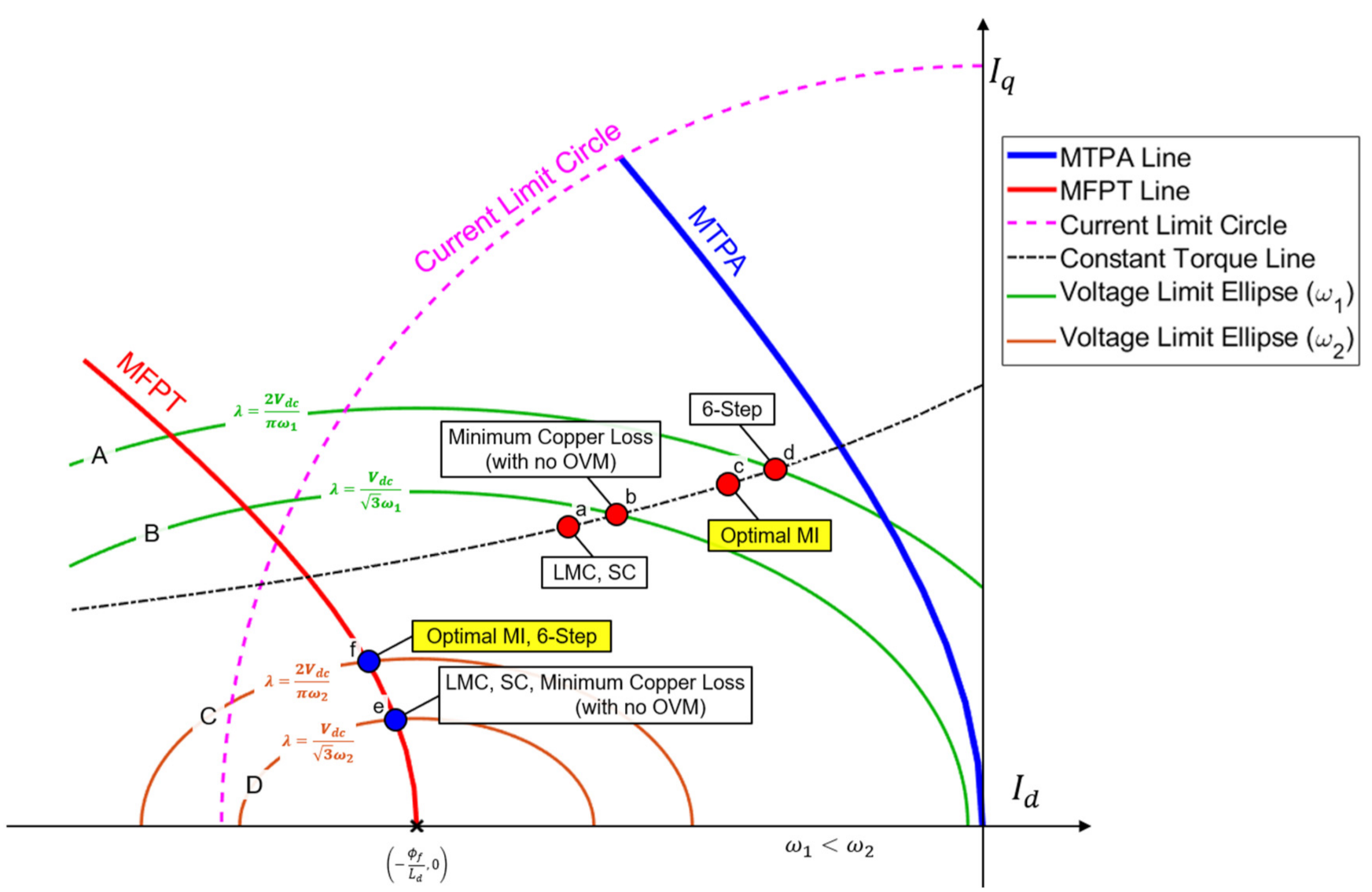
Figure 3.
Bolognani voltage overmodulation technique. is the maximum voltage that can be output from the phase angle , and if the voltage command exceeds this value, the voltage is output at a new phase angle, . Since the phase angle of the voltage is changed to an arbitrary value, the new phase voltage contains harmonics, but the magnitude of the voltage effectively applied to the motor can be increased.
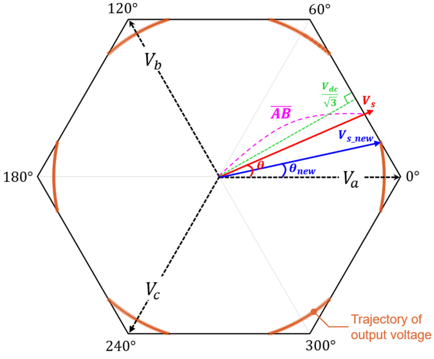
Figure 4.
Comparison of magnitudes of fundamental frequency components of command voltage and output voltage.
Figure 4.
Comparison of magnitudes of fundamental frequency components of command voltage and output voltage.
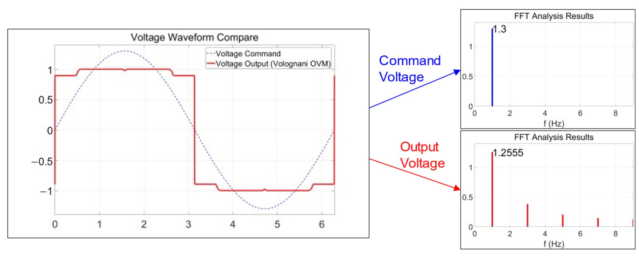
Figure 5.
Compensation of the command voltage in the nonlinear overmodulation region.
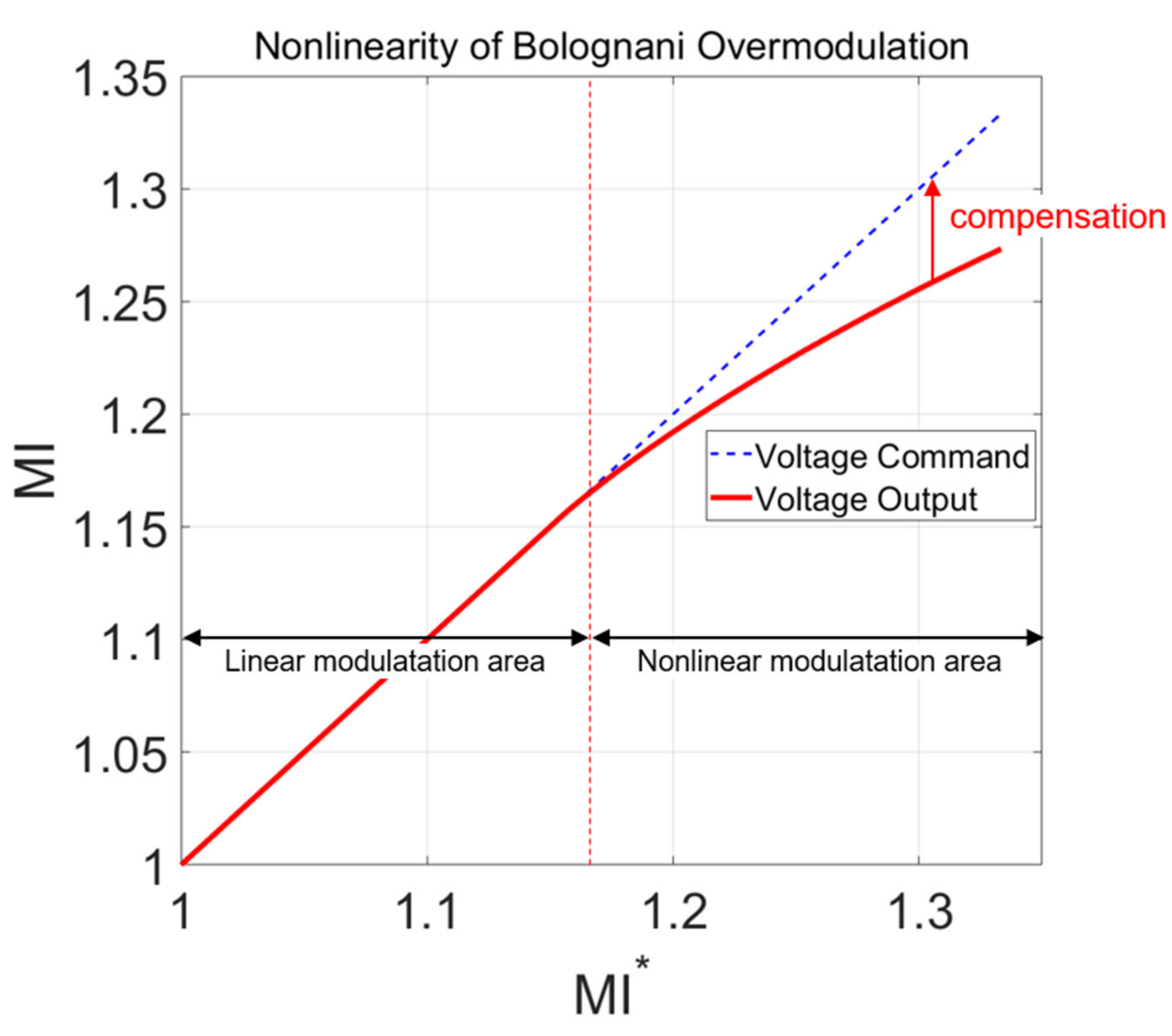
Figure 6.
Block diagram of voltage utilization optimal control algorithm.
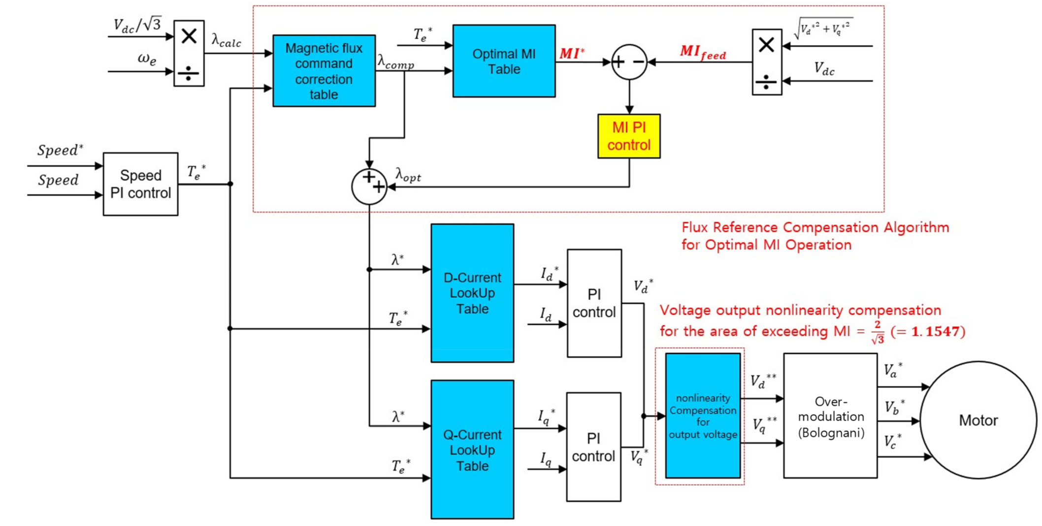
Figure 7.
Strategies for obtaining an optimal MI according to speed range.

Figure 8.
MATLAB Simulink model block diagram.

Figure 9.
Test point for observing the efficiency change on a constant torque curve.
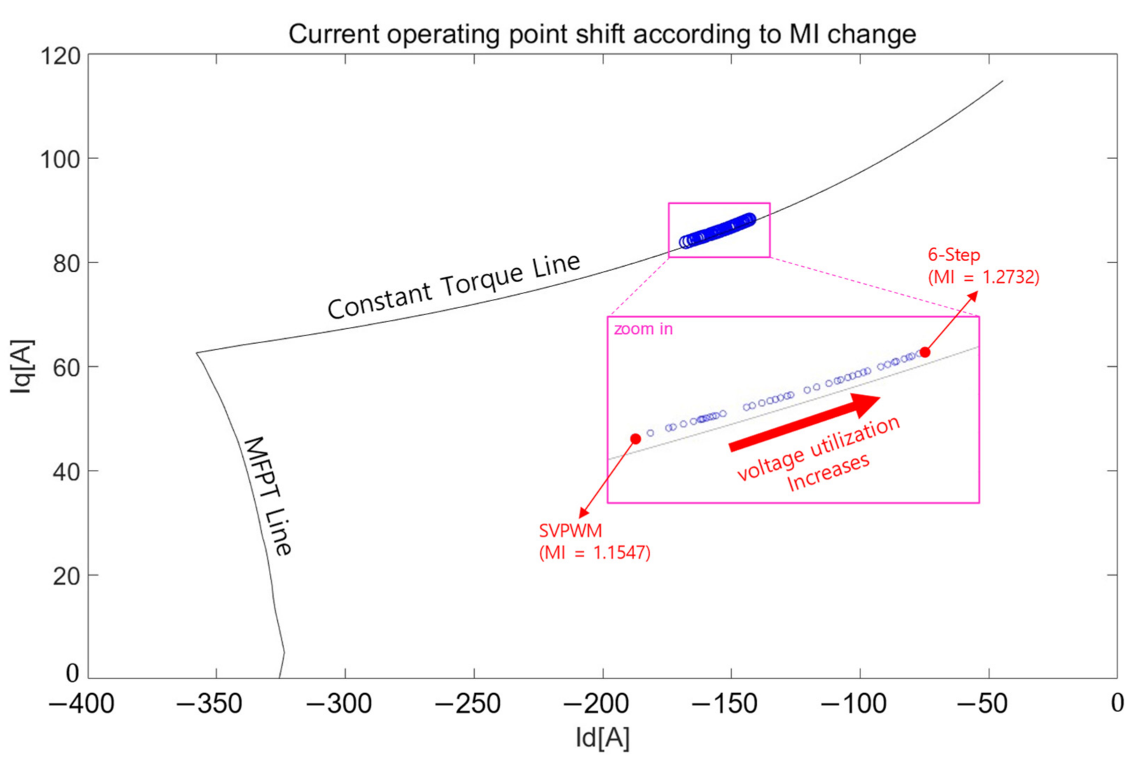
Figure 10.
Efficiency change according to overmodulation index change (CTC).
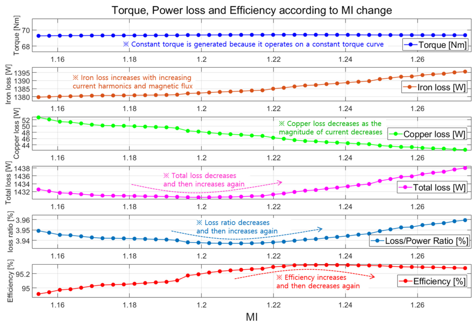
Figure 11.
Test point for observing the efficiency change on an MFPT curve.
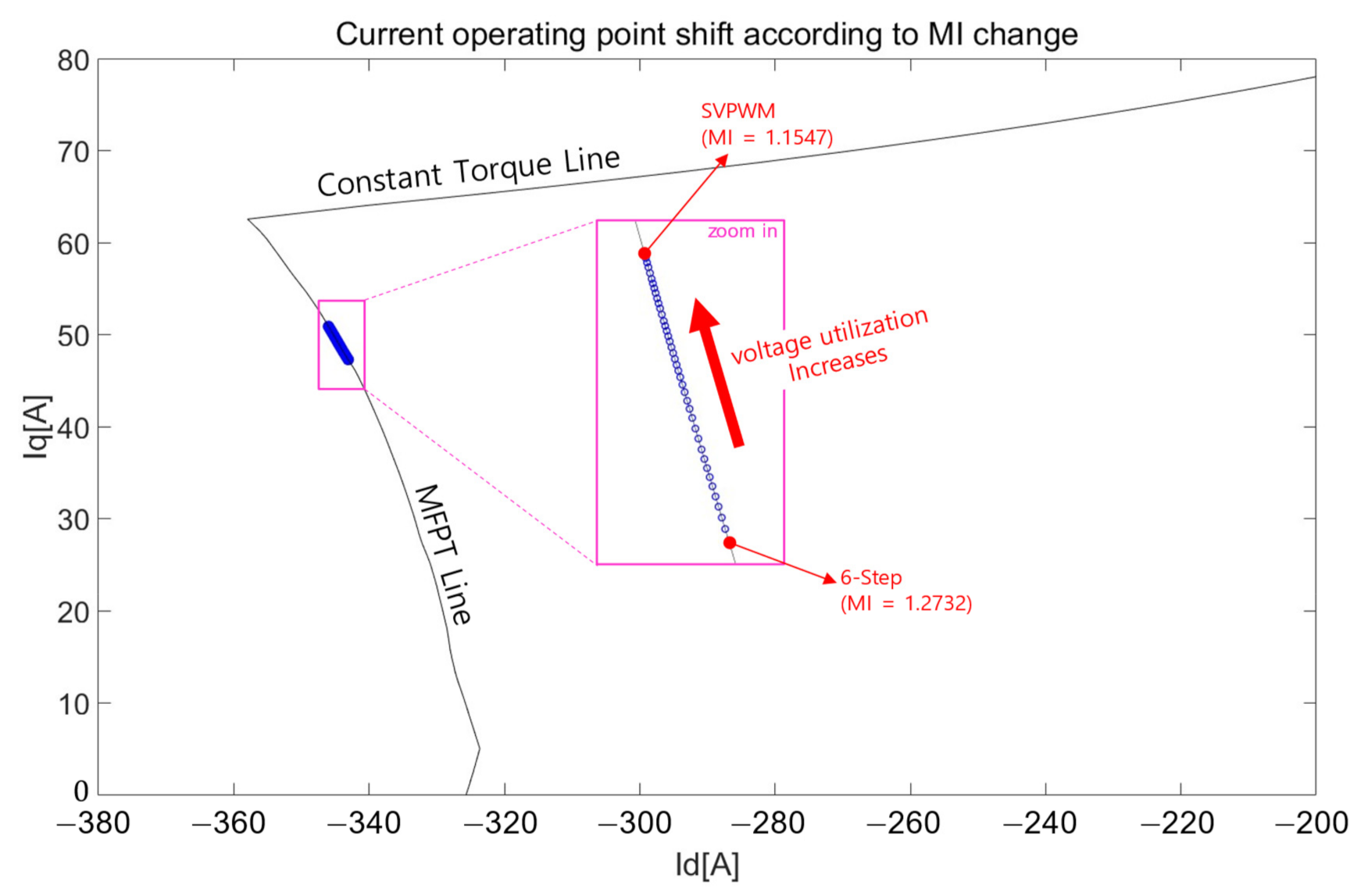
Figure 12.
Efficiency change according to overmodulation index change (MFPT).
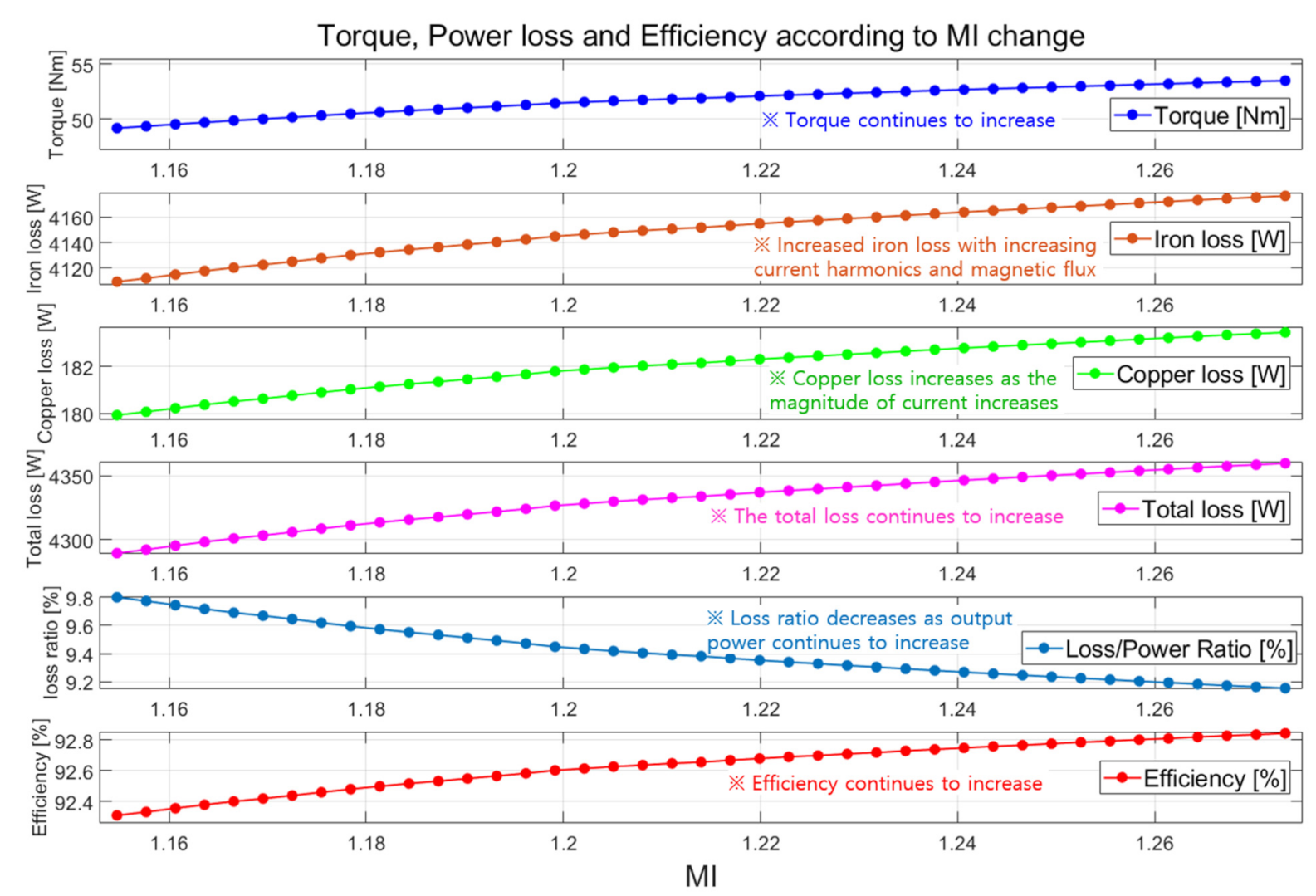
Figure 13.
Schematic diagram of dynamometer experimental equipment.
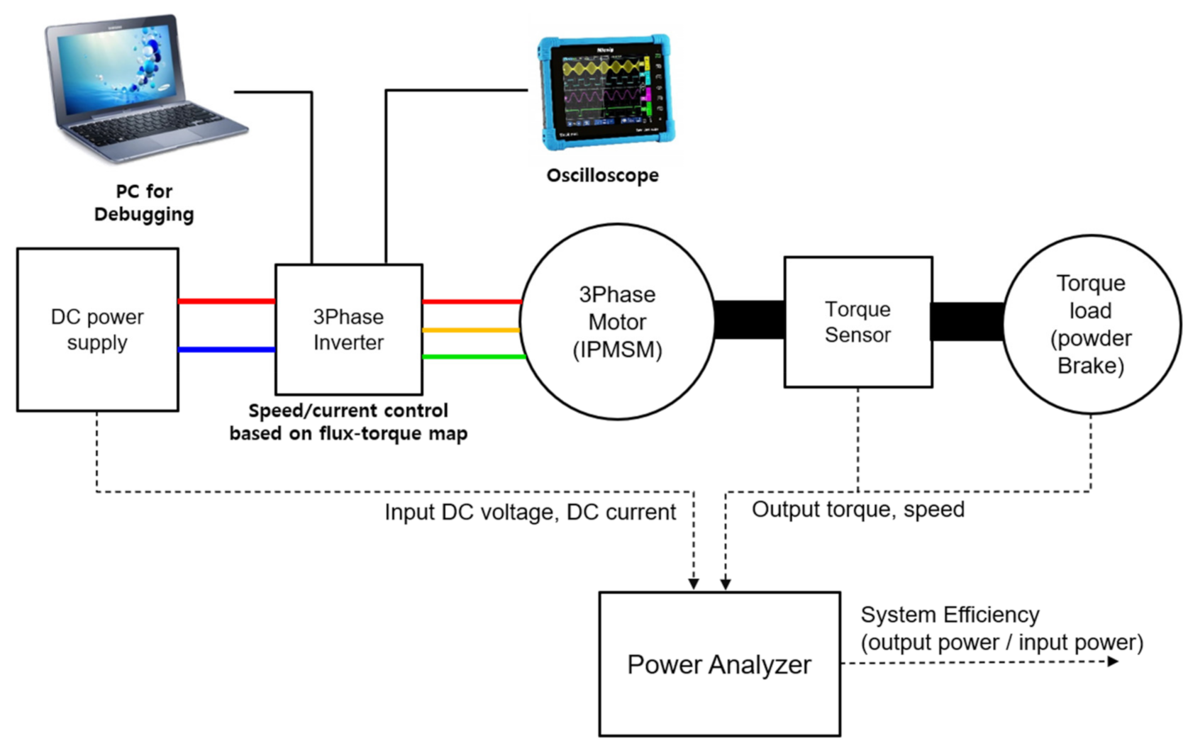
Figure 14.
Experimental results of efficiency change according to MI change.

Figure 15.
Test point used for creating an optimal MI table.
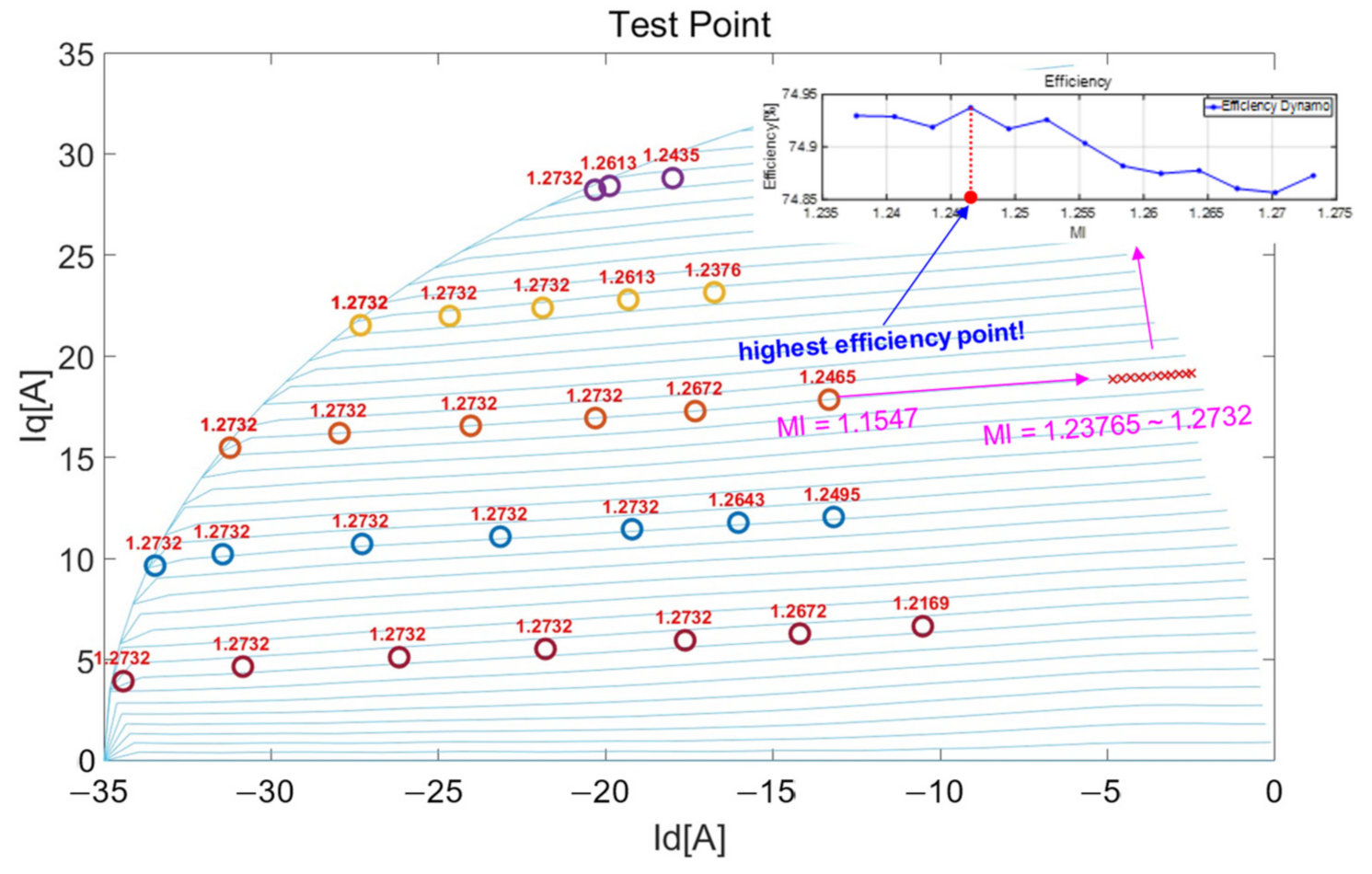
Figure 16.
Optimal MI expressed based on flux–torque command.
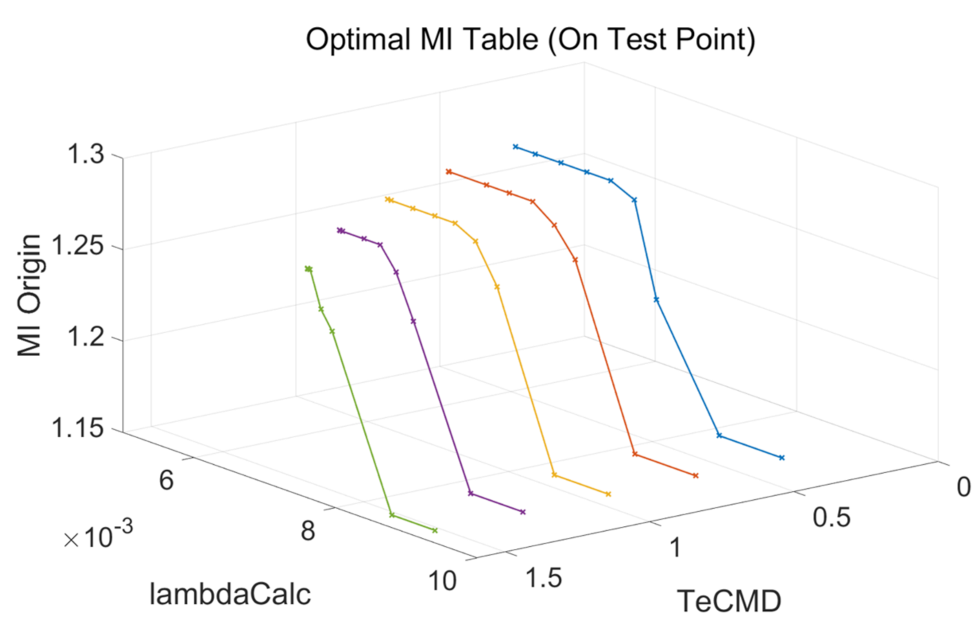
Figure 17.
Optimal MI table with increased resolution by interpolation and extrapolation.
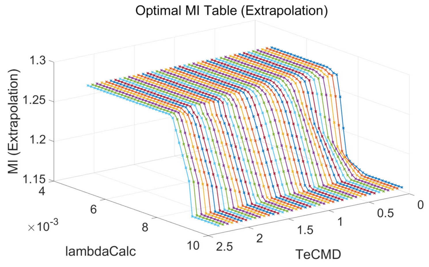
Figure 18.
Optimal MI table matched to the current operating point.

Figure 19.
Efficiency comparison of fixed MI control and optimal MI control.
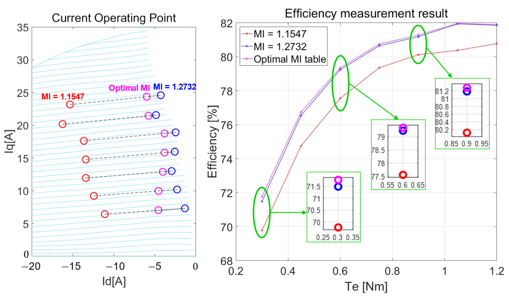
Figure 20.
Comparison results of phase current ripple of optimal MI and fixed MI.

Table 1.
Efficiency comparison results of optimal MI and fixed MI.
| Te [Nm] | Vdc [V] | Efficiency [%] | Efficiency Improvement (1.1547 vs. Optimal MI) | Efficiency Improvement (1.2732 vs. Optimal MI) | ||
|---|---|---|---|---|---|---|
| MI 1.1547 | MI 1.2732 | Optimal MI | ||||
| 0.3 | 10.3 | 69.77 | 71.49 | 71.77 (MI = 1.224) | 2.00% | 0.29% |
| 0.45 | 10.5 | 74.76 | 76.54 | 76.75 (MI = 1.237) | 1.99% | 0.21% |
| 0.6 | 10.7 | 77.55 | 79.24 | 79.35 (MI = 1.253) | 1.80% | 0.11% |
| 0.75 | 10.98 | 79.36 | 80.65 | 80.75 (MI = 1.253) | 1.40% | 0.10% |
| 0.9 | 11.25 | 80.12 | 81.18 | 81.28 (MI = 1.252) | 1.16% | 0.10% |
| 1.05 | 11.34 | 80.38 | 81.94 | 81.97 (MI = 1.256) | 1.59% | 0.03% |
| 1.2 | 11.7 | 80.78 | 81.86 | 81.89 (MI = 1.239) | 1.11% | 0.04% |
Publisher’s Note: MDPI stays neutral with regard to jurisdictional claims in published maps and institutional affiliations. |
© 2022 by the authors. Licensee MDPI, Basel, Switzerland. This article is an open access article distributed under the terms and conditions of the Creative Commons Attribution (CC BY) license (https://creativecommons.org/licenses/by/4.0/).
Share and Cite
MDPI and ACS Style
Park, J.-H.; Lim, H.-S.; Lee, G.-H.; Lee, H.-H. A Study on the Optimal Control of Voltage Utilization for Improving the Efficiency of PMSM. Electronics 2022, 11, 2095. https://doi.org/10.3390/electronics11132095
AMA Style
Park J-H, Lim H-S, Lee G-H, Lee H-H. A Study on the Optimal Control of Voltage Utilization for Improving the Efficiency of PMSM. Electronics. 2022; 11(13):2095. https://doi.org/10.3390/electronics11132095
Chicago/Turabian StylePark, Ji-Hwan, Hee-Sun Lim, Geun-Ho Lee, and Heon-Hyeong Lee. 2022. "A Study on the Optimal Control of Voltage Utilization for Improving the Efficiency of PMSM" Electronics 11, no. 13: 2095. https://doi.org/10.3390/electronics11132095
Note that from the first issue of 2016, this journal uses article numbers instead of page numbers. See further details here.