
An Efficient Adaptive Fuzzy Hierarchical Sliding Mode Control Strategy for 6 Degrees of Freedom Overhead Crane

 , ,
, ,
Abstract
:1. Introduction
2. A Model of 3D Overhead Crane with 6 Degrees of Freedom
3. Hierarchical Sliding Mode Controller for 3D Overhead Crane
4. Adaptive Fuzzy Learning Scheme
5. Results and Discussions
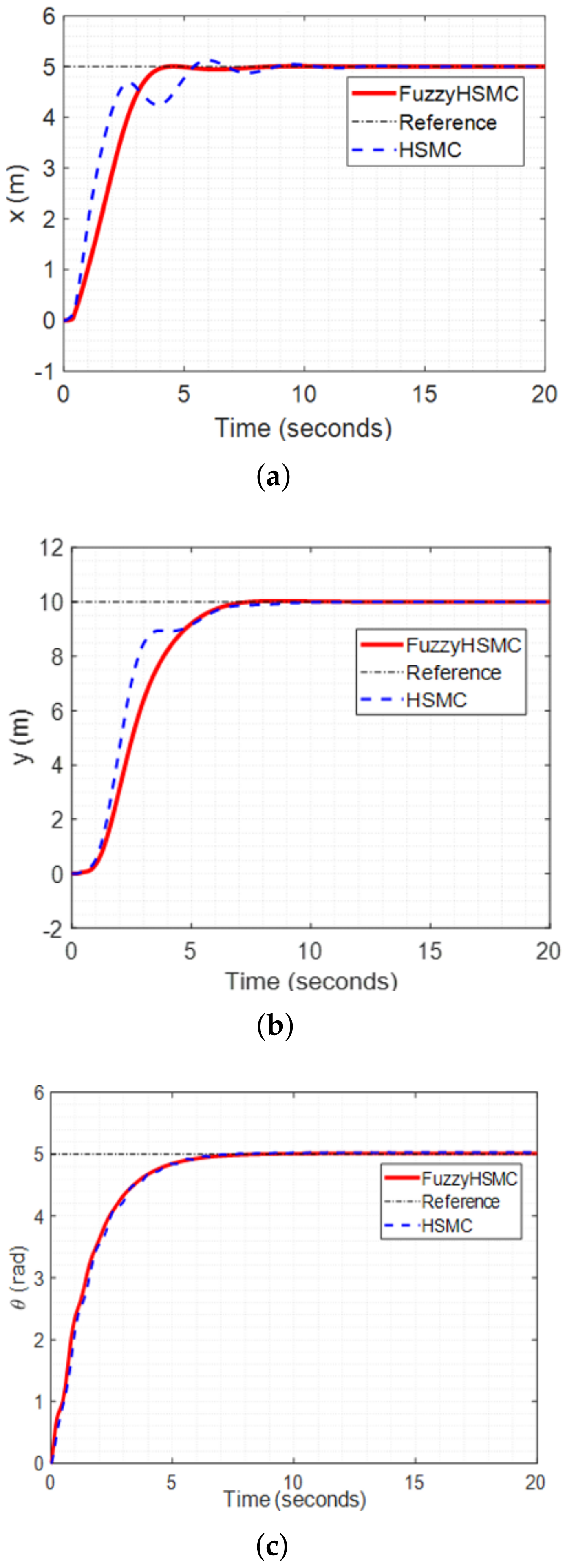
5.1. Constant Input
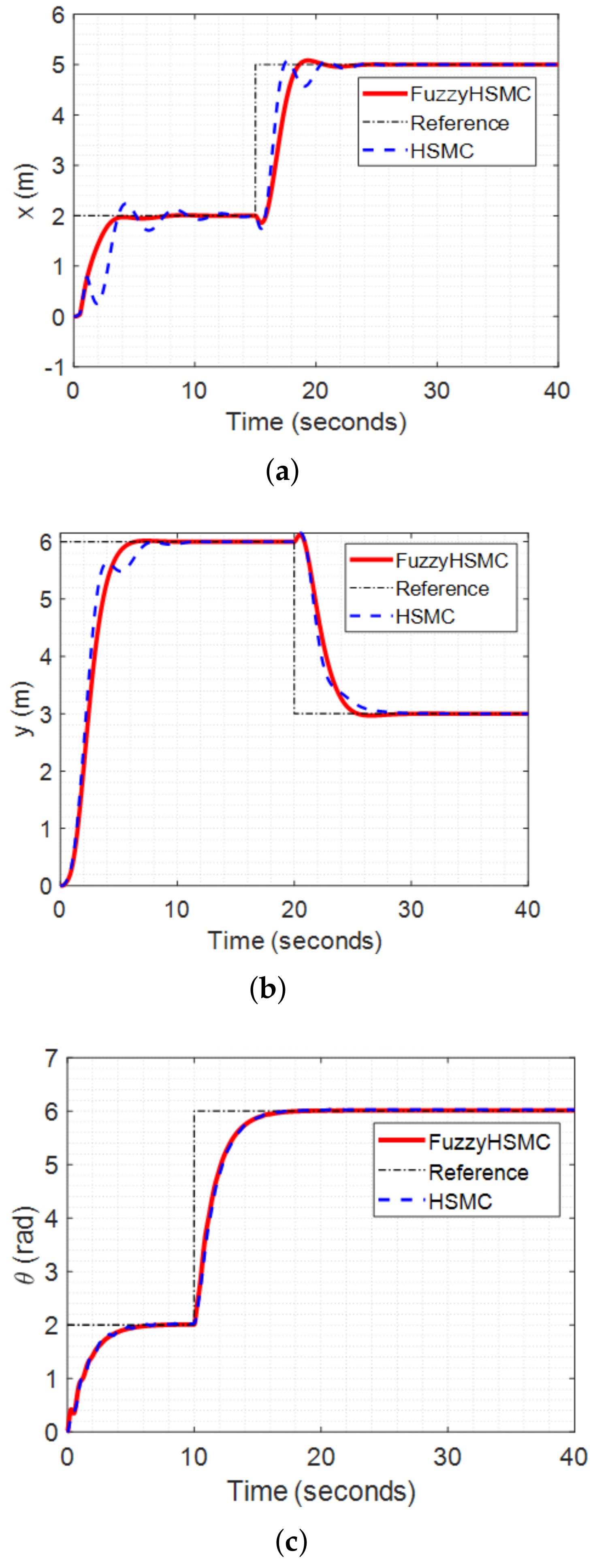
5.2. Step Input
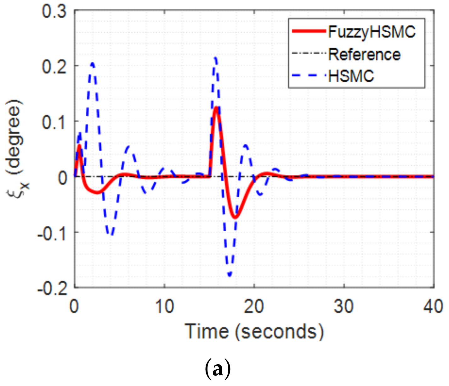
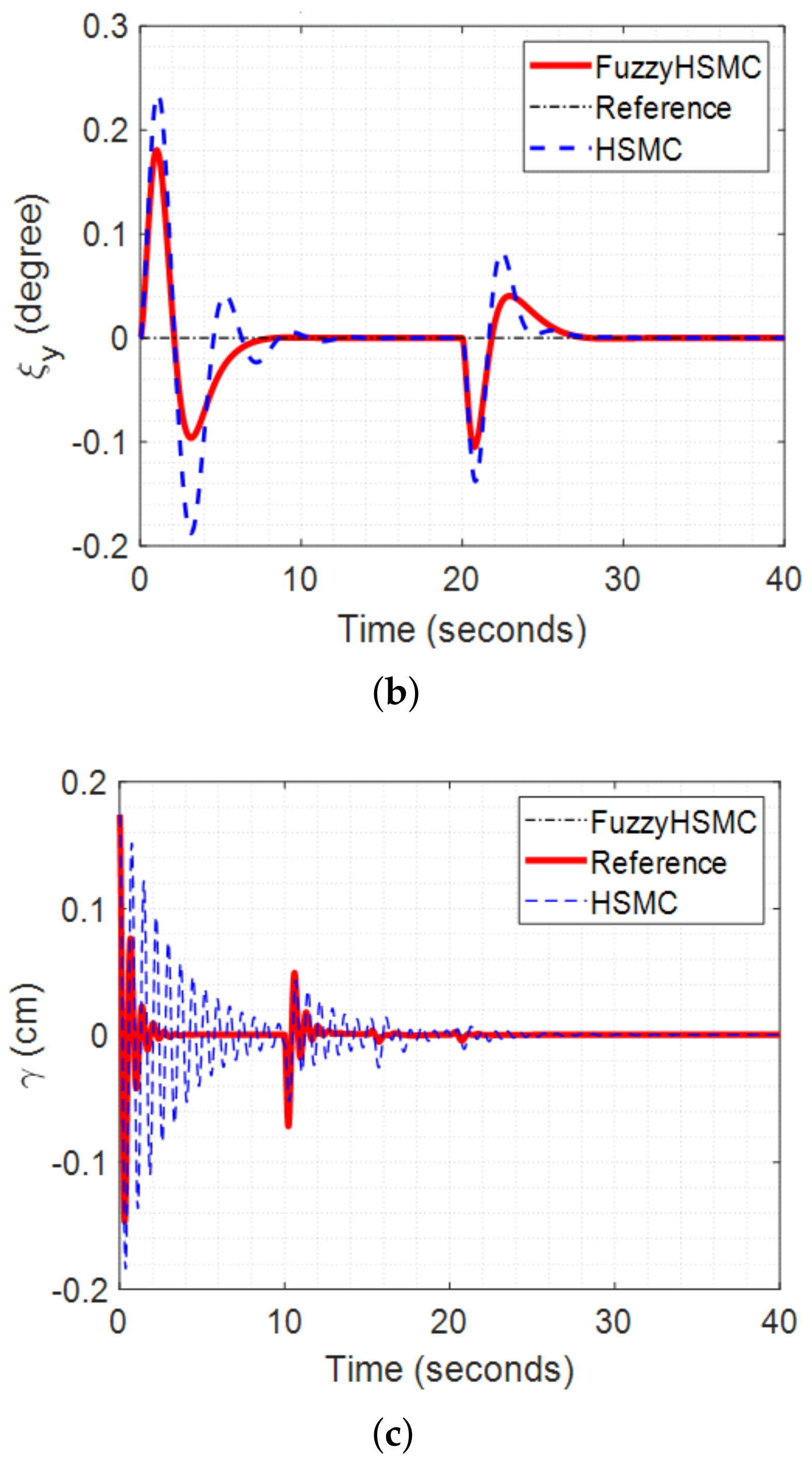
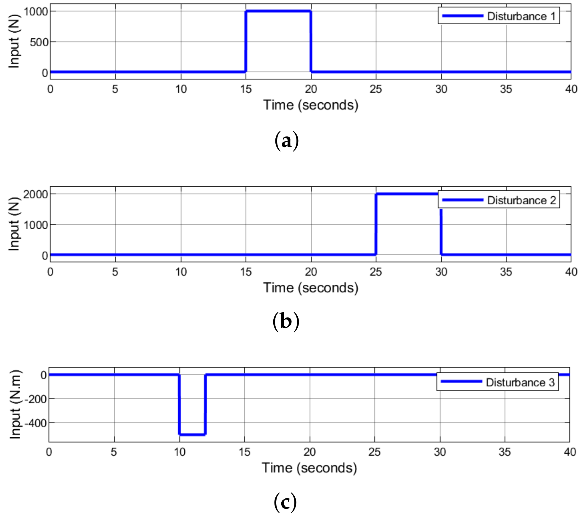
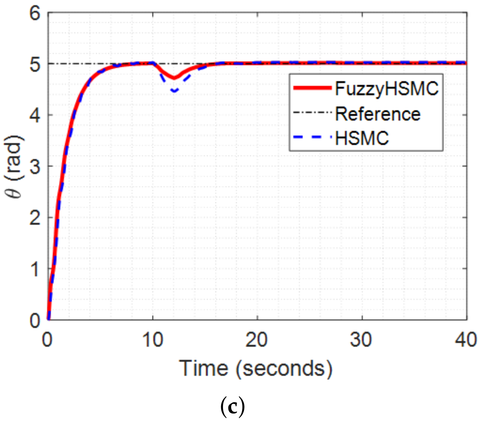
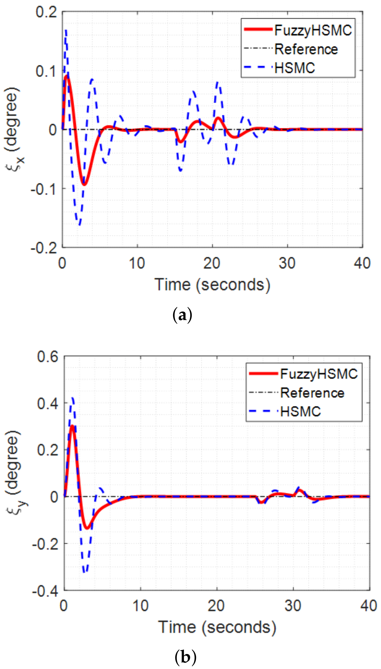
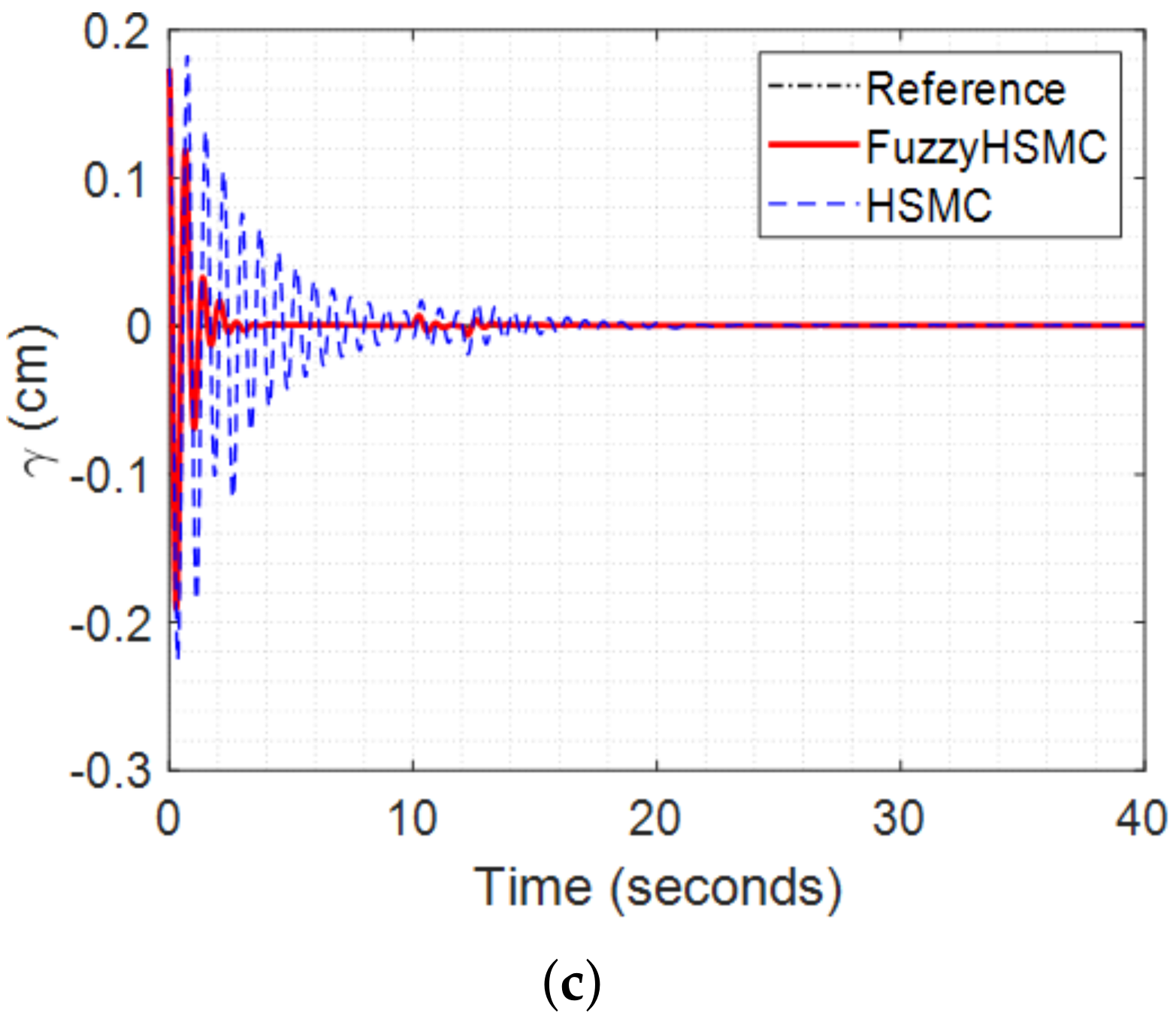
5.3. Noisy Input
6. Conclusions
Author Contributions
Funding
Conflicts of Interest
Appendix A
References
- Van Nguyen, T.; Le, H.X.; Tran, H.V.; Nguyen, D.A.; Nguyen, M.N.; Nguyen, L. An Efficient Approach for SIMO Systems using Adaptive Fuzzy Hierarchical Sliding Mode Control. In Proceedings of the 2021 IEEE International Conference on Autonomous Robot Systems and Competitions (ICARSC), Santa Maria da Feira, Portugal, 28–29 April 2021; pp. 85–90. [Google Scholar] [CrossRef]
- Li, Y.; Xi, X.; Xie, J.; Liu, C. Study and Implementation of a Cooperative Hoisting for Two Crawler Cranes. J. Intell. Robot. Syst. 2016, 83, 165–178. [Google Scholar] [CrossRef]
- Xing, X.; Liu, J. Vibration and Position Control of Overhead Crane with Three-Dimensional Variable Length Cable Subject to Input Amplitude and Rate Constraints. IEEE Trans. Syst. Man Cybern. Syst. 2021, 51, 4127–4138. [Google Scholar] [CrossRef]
- Campeau-Lecours, A.; Foucault, S.; Laliberté, T.; Mayer-St-Onge, B.; Gosselin, C. A Cable-Suspended Intelligent Crane Assist Device for the Intuitive Manipulation of Large Payloads. IEEE/ASME Trans. Mechatron. 2016, 21, 2073–2084. [Google Scholar] [CrossRef] [Green Version]
- Rigatos, G.; Siano, P.; Abbaszadeh, M. Nonlinear H-infinity control for 4-DOF underactuated overhead cranes. Trans. Inst. Meas. Control 2018, 40, 2364–2377. [Google Scholar] [CrossRef]
- Mahapatra, S.; Subudhi, B. Design and experimental realization of a backstepping nonlinear H∞ control for an autonomous underwater vehicle using a nonlinear matrix inequality approach. Trans. Inst. Meas. Control 2018, 40, 3390–3403. [Google Scholar] [CrossRef]
- Le, H.X.; Nguyen, L.; Thiyagarajan, K. A Dynamic Surface Controller based on Adaptive Neural Network for Dual Arm Robots. In Proceedings of the 2020 15th IEEE Conference on Industrial Electronics and Applications (ICIEA), Kristiansand, Norway, 9–13 November 2020; pp. 555–560. [Google Scholar]
- Nguyen, T.V.; Thai, N.H.; Pham, H.T.; Phan, T.A.; Nguyen, L.; Le, H.X.; Nguyen, H.D. Adaptive Neural Network-Based Backstepping Sliding Mode Control Approach for Dual-Arm Robots. J. Control Autom. Electr. Syst. 2019, 30, 512–521. [Google Scholar] [CrossRef] [Green Version]
- Vu, Q.V.; Dinh, T.A.; Nguyen, T.V.; Tran, H.V.; Le, H.X.; Pham, H.V.; Kim, T.D.; Nguyen, L. An Adaptive Hierarchical Sliding Mode Controller for Autonomous Underwater Vehicles. Electronics 2021, 10, 2316. [Google Scholar] [CrossRef]
- Pham, D.T.; Nguyen, T.V.; Le, H.X.; Nguyen, L.; Thai, N.H.; Phan, T.A.; Pham, H.T.; Duong, A.H.; Bui, L.T. Adaptive neural network based dynamic surface control for uncertain dual arm robots. Int. J. Dyn. Control 2020, 8, 824–834. [Google Scholar] [CrossRef] [Green Version]
- Hoang, U.T.T.; Le, H.X.; Thai, N.H.; Pham, H.V.; Nguyen, L. Consistency of Control Performance in 3D Overhead Cranes under Payload Mass Uncertainty. Electronics 2020, 9, 657. [Google Scholar] [CrossRef] [Green Version]
- Le, V.A.; Le, H.X.; Nguyen, L.; Phan, M.X. An Efficient Adaptive Hierarchical Sliding Mode Control Strategy Using Neural Networks for 3D Overhead Cranes. Int. J. Autom. Comput. 2019, 16, 614–627. [Google Scholar] [CrossRef] [Green Version]
- Le, H.X.; Le, A.V.; Nguyen, L. Adaptive fuzzy observer based hierarchical sliding mode control for uncertain 2D overhead cranes. Cyber-Phys. Syst. 2019, 5, 191–208. [Google Scholar] [CrossRef]
- Fu, Y.; Sun, N.; Yang, T.; Qiu, Z.; Fang, Y. Adaptive Coupling Anti-Swing Tracking Control of Underactuated Dual Boom Crane Systems. IEEE Trans. Syst. Man Cybern. Syst. 2021, 3, 1–13. [Google Scholar] [CrossRef]
- Xu, W.; Zheng, X.; Liu, Y.; Zhang, M.; Luo, Y. Adaptive dynamic sliding mode control for overhead cranes. In Proceedings of the 2015 34th Chinese Control Conference (CCC), Hangzhou, China, 28–30 July 2015; pp. 3287–3292. [Google Scholar]
- Li, Y.; Zhou, S.; Zhu, H. A backstepping controller design for underactuated crane system. In Proceedings of the 2018 Chinese Control and Decision Conference (CCDC), Shenyang, China, 9–11 June 2018; pp. 2895–2899. [Google Scholar] [CrossRef]
- Tsai, C.C.; Wu, H.L.; Chuang, K.H. Backstepping aggregated sliding-mode motion control for automatic 3D overhead cranes. In Proceedings of the 2012 IEEE/ASME International Conference on Advanced Intelligent Mechatronics (AIM), Kaohsiung, Taiwan, 11–14 July 2012; pp. 849–854. [Google Scholar] [CrossRef]
- Yang, T.; Sun, N.; Fang, Y. Adaptive Fuzzy Control for a Class of MIMO Underactuated Systems with Plant Uncertainties and Actuator Deadzones: Design and Experiments. IEEE Trans. Cybern. 2021, 1–14. [Google Scholar] [CrossRef] [PubMed]
- Yang, T.; Sun, N.; Fang, Y. Neuroadaptive Control for Complicated Underactuated Systems with Simultaneous Output and Velocity Constraints Exerted on Both Actuated and Unactuated States. IEEE Trans. Neural Netw. Learn. Syst. 2021, 1–11. [Google Scholar] [CrossRef] [PubMed]
- Wang, W.; Yi, J.; Zhao, D.; Liu, D. Design of a stable sliding-mode controller for a class of second-order underactuated systems. IEE Proc.-Control Theory Appl. 2004, 151, 683–690. [Google Scholar] [CrossRef] [Green Version]
- Mahjoub, S.; Mnif, F.; Derbel, N. Second-order sliding mode approaches for the control of a class of underactuated systems. Int. J. Autom. Comput. 2015, 12, 134–141. [Google Scholar] [CrossRef]
- Zadeh, L.A. Is there a need for fuzzy logic? Inf. Sci. 2008, 178, 2751–2779. [Google Scholar] [CrossRef]
- Yang, T.; Chen, H.; Sun, N.; Fang, Y. Adaptive Neural Network Output Feedback Control of Uncertain Underactuated Systems with Actuated and Unactuated State Constraints. IEEE Trans. Syst. Man Cybern. Syst. 2021, 1–17. [Google Scholar] [CrossRef]
- Yue, M.; An, C.; Du, Y.; Sun, J. Indirect adaptive fuzzy control for a nonholonomic/underactuated wheeled inverted pendulum vehicle based on a data-driven trajectory planner. Fuzzy Sets Syst. 2016, 290, 158–177. [Google Scholar] [CrossRef]
- Al-saedi, M.I. Enhancing the Feedforward –Feedback Controller for Nonlinear Overhead Crane Using Fuzzy logic controller. IOP Conf. Ser. Mater. Sci. Eng. 2020, 745, 012074. [Google Scholar] [CrossRef]
- Zdesar, A.; Cerman, O.; Dovzan, D.; Husek, P.; Skrjanc, I. Fuzzy Control of a Helio-Crane. J. Intell. Robot. Syst. 2013, 72, 497–515. [Google Scholar] [CrossRef]
- Shi, H.; Li, G.; Bai, X.; Huang, J. Research on Nonlinear Control Method of Underactuated Gantry Crane Based on Machine Vision Positioning. Symmetry 2019, 11, 987. [Google Scholar] [CrossRef] [Green Version]


| Parameter () | ||||
|---|---|---|---|---|
| −1 | 0 | 1 | ||
| −1 | 2 | 1 | 0 | |
| 0 | 1 | 0 | −1 | |
| 1 | 0 | −1 | −2 | |
| Parameter | Value | Unit |
|---|---|---|
| 2316.5 | kg | |
| 500 | kg | |
| 371.9 | kg | |
| J | 180 | kg·m |
| r | 0.31 | m |
| g | 9.81 | m/s |
| 300,000 | N/m | |
| 0.01 | m | |
| 350 | N·m/s | |
| 310 | N·m/s | |
| 170 | N·m/s | |
| 260 | N·m/s |
| Parameter | Value |
|---|---|
| diag([0.6 0.5 4]) | |
| diag([1.2 1.5 1]) | |
| diag([0.6 0.2 1.3]) | |
| diag([2.4 0.7 0.8]) | |
| diag([0.2 1.6 0.1]) | |
| diag([4 1.6 0.6]) | |
| diag([3 5 0.05]) | |
| diag([1 0.5 0.1]) | |
| diag([5 1.6 0.15]) |
Publisher’s Note: MDPI stays neutral with regard to jurisdictional claims in published maps and institutional affiliations. |
© 2022 by the authors. Licensee MDPI, Basel, Switzerland. This article is an open access article distributed under the terms and conditions of the Creative Commons Attribution (CC BY) license (https://creativecommons.org/licenses/by/4.0/).
Share and Cite
Pham, H.V.; Hoang, Q.-D.; Pham, M.V.; Do, D.M.; Phi, N.H.; Hoang, D.; Le, H.X.; Kim, T.D.; Nguyen, L. An Efficient Adaptive Fuzzy Hierarchical Sliding Mode Control Strategy for 6 Degrees of Freedom Overhead Crane. Electronics 2022, 11, 713. https://doi.org/10.3390/electronics11050713
Pham HV, Hoang Q-D, Pham MV, Do DM, Phi NH, Hoang D, Le HX, Kim TD, Nguyen L. An Efficient Adaptive Fuzzy Hierarchical Sliding Mode Control Strategy for 6 Degrees of Freedom Overhead Crane. Electronics. 2022; 11(5):713. https://doi.org/10.3390/electronics11050713
Chicago/Turabian StylePham, Hung Van, Quoc-Dong Hoang, Minh Van Pham, Dung Manh Do, Nha Hoang Phi, Duy Hoang, Hai Xuan Le, Thai Dinh Kim, and Linh Nguyen. 2022. "An Efficient Adaptive Fuzzy Hierarchical Sliding Mode Control Strategy for 6 Degrees of Freedom Overhead Crane" Electronics 11, no. 5: 713. https://doi.org/10.3390/electronics11050713