
Resilient Networked Control of Inverter-Based Microgrids against False Data Injections
by
Mohammad Reza Khalghani
1,*, 
Vishal Verma
2,
Sarika Khushalani Solanki
2 and
Jignesh M. Solanki
2 1
Department of Electrical and Computer Engineering, Florida Polytechnic University, Lakeland, FL 33805, USA
2
Lane Department of Computer Science and Electrical Engineering, West Virginia University, Morgantown, WV 26506, USA
*
Author to whom correspondence should be addressed.
Electronics 2022, 11(5), 780; https://doi.org/10.3390/electronics11050780
Submission received: 31 January 2022
/
Revised: 12 February 2022
/
Accepted: 15 February 2022
/
Published: 3 March 2022
(This article belongs to the Special Issue Security of Cyber-Physical Systems)
Abstract
:Inverter-based energy resource is a fast emerging technology for microgrids. Operation of micorgrids with integration of these resources, especially in an islanded operation mode, is challenging. To effectively capture microgrid dynamics and also control these resources in islanded microgrids, a heavy cyber and communication infrastructure is required. This high reliance of microgrids on cyber interfaces makes these systems prone to cyber-disruptions. Hence, the hierarchical control of microgrids, including primary, secondary, and tertiary control, needs to be developed to operate resiliently. This paper shows the vulnerability of microgrid control in the presence of False Data Injection (FDI) attack, which is one type of cyber-disruption. Then, this paper focuses on designing a resilient secondary control based on Unknown Input Observer (UIO) against FDI. The simulation results show the superior performance of the proposed controller over other standard controllers.
1. Introduction
Due to the environmentally friendly characteristics of renewable energies and distributed energy resources, integrating these energy resources into distribution grids is growing significantly. There is an ongoing shift of system configuration from traditional distribution grids to small distributed and controllable microgrids. Microgrids can locally supply loads through distributed energy resources that include renewable energy resources and operate in grid-connected and islanded modes. Islanded mode of operation allows the microgrid to provide energy without the support of the main grid, which is critically important when the main grid cannot exchange energy with other local microgrids, such as during natural hazards and extreme weather events.
Sustaining the islanded operation of microgrids is challenging since the grid relies on a limited number of energy resources. This challenging task can be addressed by utilizing hierarchical control methods comprised of primary, secondary, and tertiary controls [1]. The primary control response is the immediate regulation of power output by the governor or electronic controller in response to changes in the grid frequency. Considering the limited capability of the primary control loop to address frequency changes, it is necessary to design the secondary control to control the grid dynamics [2]. Secondary control is a supervisory control that utilizes measurements communicated through cyber systems to capture and control fast microgrid dynamics. Hierarchical control can coordinate inverter-based energy resources to effectively track the sudden load changes and nondispatchable generators. Tertiary control focuses on optimal power flow between the main grid and microgrids, which is not within the scope of this paper.
Since the secondary control heavily relies on communications and cyber infrastructures in a closed control loop, it can be labeled as a networked control system [3]. Similar to all networked control systems, the secondary control of microgrids is vulnerable to cyber threats. Although there is a wide variety of cyberattacks, more common types are Denial-of-Service (DoS) and False Data Injection (FDI). The DoS targets the availability of machines or networks to temporarily or indefinitely distort the service to its intended users. The FDI manipulates the data exchanges throughout the network, which misleads the control center and disturbs the system operation [3,4].
Many researchers proposed a secure secondary control for microgrids. In [5], the authors review cybersecurity threats and introduce cyber attack prevention, detection, and response measures for the integration of inverter-based resources to grids. Researchers in [6] focus on the security of distributed secondary control of microgrids by proposing a Weighted Mean Subsequence Reduced algorithm at each inverter-based resource. A distributed secondary control based on a consensus algorithm is proposed to control the frequency of an islanded microgrid in [7]. Another distributed control strategy was developed in [8] where the authors designed a resilient control against cyber attacks on communication links, local controllers, and master controllers of microgrids. Also, researchers in [9] proposed a distributed control strategy based on blockchain to enhance cyber vulnerability of microgrids equipped with distributed energy resources. [10] constructs an attack detector based on the stable kernel representation of an islanded microgrid. A resilient secondary control method is proposed in [11] that mitigates Denial-of-Service (DoS) attacks from inverter-based microgrids. This proposed control method is mode-dependent and assumes that the random DoS attack follows a homogeneous Markov process. Another distributed control method is developed for islanded microgrids in [12] to secure the system from malicious attacks on the communication network, including links and nodes. The authors in [13] present secondary control for energy storage systems to control the frequency and voltage of an islanded microgrid. This control strategy uses an event-trigger scheme to lower the communication burden in the network. Most research work does not focus on inverter-based microgrids and additionally does not focus on a resilient controller that considers fast dynamics, especially under cyber disruptions.
This paper focuses on designing a resilient secondary controller against false data injection for an islanded microgrid equipped with inverter-based energy resources. The rest of the paper is organized as follows. Section 2 presents a general model for inverter-based microgrid model. The proposed secondary controller based on Unknown Input Observer (UIO) is described in Section 3. A vulnerability analysis of the islanded microgrid against FDI is elaborated in Section 4. Simulation and results are demonstrated in Section 5, and the conclusion is presented in Section 6.
2. Model of Inverter-Based Microgrids
This section introduces the inverter-based microgrid model equipped with primary control. Also, this section proposes the optimal resilient secondary control for the islanded microgrid.
2.1. The Microgrid State-Space Representation
This islanded microgrid model includes three major elements of inverters, grid topology, and loads. Inverters dynamics cover output filter, coupling inductor, power-sharing controller, and current and voltage controllers. Each inverter has a separate reference frame, e.g., axis for ith inverter, whose rotating frequency is tuned by its power-sharing controller. Rotating frequency denotes the reference frame of one of the microgrid inverters. A common reference frame with axis and rotating frequency characterize the loads and the network’s dynamic equations. Through the following transformation matrix, other inverters’ reference frames are translated to the common reference frame [14]:
where is the angle of the reference frame of ith inverter with respect to the common reference frame. In this paper, all inverters are Voltage Source Inverters (VSI) which are usually applied to interface distributed generators (DGs) to grids.
2.1.1. VSI State-Space Model
Figure 1 shows that the DG inverter control process has three different parts, such as voltage, current, and power control loops. The power control loop regulates the magnitude and frequency for the fundamental component of the inverter’s voltage according to the droop characteristic set for the active and reactive powers. Voltage and current controllers are utilized to eliminate high-frequency disturbances and obtain proper damping for the output filter [14,15]. Since frequency control of this islanded microgrid is within the scope of this paper, we only describe the VSI power controller (not voltage and current controllers). The detailed model can be learned from [14,16].
Utilizing the droop control for DG inverters, we mimic the governor behavior of synchronous generators in power systems. When there is a load rise, the microgrid frequency is reduced. Besides, when there is a voltage decrease, the reactive power is regulated proportionally. The power control diagram of VSIs is shown in Figure 2. Examining Figure 2, instantaneous active and reactive power are provided from the measured current and voltage in frame as in (3) and (4):
Also, these instantaneous power elements are passed through low-pass filters with cut-off frequency to obtain the fundamental real and reactive power as in (5) and (6):
The artificial droop can share active and reactive powers in the inverter frequency. As seen in (7), the frequency is set based on the droop coefficient , and the phase is set by the frequency integration. indicates the nominal frequency set-point, and indicates the inverter reference frame angle with nominal rotating frequency [14]:
Similar to active power, an artificial droop is used to share reactive power through specifying the output voltage magnitude, which is set to the d-axis of the inverter reference frame (the q-axis reference is set to zero) as in (8):
The droop coefficients and are provided using the maximum and minimum limits of frequency and voltage magnitude as:
As expressed earlier, one of the inverters’ reference frames is picked as the common frame to build-up the complete model on a common reference frame. An angle is specified for each inverter as in (10) to transfer the variables of other inverters into the common reference frame:
where denotes the rated frequency set-point for each inverter [17]. As seen in (10), all inverter angle dynamics are a function of the first inverter active power . After considering dynamics of voltage and current controllers and reorganizing all equations, the combined small-signal model for “s” number of DG inverters on a common reference frame is as in (11) and (12):
where and .
2.1.2. Network Model
It is assumed that the islanded microgrid here has n lines, m nodes, s inverters, and p loads, as shown in Figure 3. The dynamic equations of line current of ith line connected between nodes j and k on the common reference frame are obtained as (13) and (14) [14]:
Therefore, the small-signal state-space representation of the microgrid is obtained as in (15):
2.1.3. Load Model
The dynamic equation for the resistive and inductive load connected at the ith node is obtained in (16):
Therefore, the small-signal state-space representation of loads is generally obtained as in (18):
2.1.4. Complete Microgrid Model
The microgrid model is obtained by augmenting all these modules of VSI inverters, network lines, and loads together as in (19):
where are microgrid characteristic matrices and [17] can be referred for more information. With this microgrid’s state-space model, we can design an optimal secondary control for this system and enhance the primary control performance.
2.2. Secondary Control of the Inverter-Based Microgrid
To apply an optimal control based on Linear Quadratic Regulator (LQR), we need to ensure the pair is controllable; otherwise, designing such controllers for this system is not possible. However, this system is not controllable since the small-signal transient, and the steady-state responses obtained from the first state is zero () [18]. Therefore, this state must be skipped by removing the corresponding row and column in A and B or using the minimum realization technique for this system. After making the reduced-order model, we can utilize the LQR controller on the microgrid model. The microgrid eigenvalues with and without the state corresponding to are shown in Table 1.
3. The Proposed Control Method
Standard controllers based on observes apply the entire grid states for the estimation and control procedure. Frequency deviation , which is one of the states in microgrid model, reflects frequency distortion because of intermittent behavior of renewable energy sources, loads, and any cyber anomalies in the system. Secondary controllers are often designed to guarantee the frequency stability of grids. We utilize a combined UIO and LQR controllers formed in two layers to control the microgrid. The first layer estimates the microgrid states and detects the UIs using (19). The second layer decreases the frequency discrepancy using (30)–(32).
3.1. Design of Unknown Input Observer
In UIO, the states are separated into two groups of states: states corresponding to known inputs, and states corresponding to unknown inputs, [19]. Here, state indicates the frequency discrepancy subject to the UI. Now, we can independently estimate both groups of states, including and , and ultimately and identify the UI. In this case, the frequency deviation does not distort the state estimation as well as the frequency regulation of the microgrid. For separating the states to two groups, a nonsingular matrix is determined where N is the arbitrary matrix selected such that is cannot be singular [20]. This transition matrix is multiplied to both sides of (19) to obtain its equivalent representation (20). Using this representation, we obtain another model representation with and , and new constant characteristic matrices specified in (21):
Further, the states subject to the UI are eliminated to find microgrid model free from unknown input as in (22) [20]:
Assuming can be attained from the measurement output , (22) can be reorganized to a linear representation. The transfer matrix is comprised of , which is a full-column rank matrix, and , which is an arbitrary matrix defined such that U is a nonsingular matrix. Therefore, we have with and . If the measurement equations in (22) is multiplied by , we obtain (23) and (24):
Substituting (23) in (22) and merging it with (24), we obtain (25) with revised state matrix of , modified measurement matrix , modified measurement vector , and :
A Luenberger observer can be developed for this microgrid, in case the pair is observable. The observability conditions of this microgrid is reviewed in [20]. The Luenberger observer with for is designed as in (26) to estimate with :
where and the Luenberger observer coefficient matrix L is calculated from solving the discrete Riccati equation . Also, solves the algebraic Riccati equation that reduces the steady-state error covariance . Now, all estimated states can be found in (27) using (23) and (26):
where . This indicates that the frequency discrepancy is estimated from measured data and remaining estimated states .
3.2. Unknown Input Compensator Design
The UI compensator is developed by , which is utilized in the closed-loop control of the microgrid matrix . is an optimized state feedback coefficient designed to guarantee that the Eigenvalues of fall within stable control region of the microgrid. To design this compensator coefficient, the pair must be controllable that means the rank of the controlability matrix is equal to the rank of microgrid model, or . In the second layer, the optimal compensator coefficient is obtained using input and the estimated microgrid states in (27) to minimize the performance index J in (30). and are weight matrices for control performance and input energy respectively, in (30). If , we have the proposed control law , which is a linear combination of the detected unknown inputs with , and the compensator coefficient in (31). The first term of the proposed control law is obtained from (32) to optimize the performance index J. In Equation (32), implies the unique positive-definite solution of discrete-time algebraic Riccati equation in (30) specified as . The second term of the proposed control law is the detected unknown inputs subtracted from the first term of the proposed control law to eliminate the UI. The diagram of the proposed control strategy is shown in Figure 4:
4. Vulnerability Analysis of Microgrids with Inverter-Based Resources
This section shows the vulnerability of microgrid control based on the secondary control design of the microgrid model obtained in Section 2. According to Equation (10), all inverter angle dynamics are direct functions of the first inverter active power in this model, which is introduced as (desired) reference frequency of inverters in some papers [21]. All droop gains, also called the active power sharing gains, including , are selected based on the microgrid’s power rating of energy resources. Typically, these active power sharing gains are chosen as the inverse proportion of the nominal power to guarantee the accuracy of active power-sharing, i.e., . If this proportion ratio is distorted, it may destabilize the microgrid.
Disclosing and injecting the data packets of the first inverter active power can enormously distort the stability and performance of the entire grid for three critical reasons:
- Stealthy FDIs always severely impact systems since this class of cyber attacks cannot be easily identified [22]. Most detecting methods fail correctly to discover the stealthy FDIs since they mainly rely on residual-based detection that may not trigger the alarm in the presence of this cyber attack type;
- Islanded microgrids have limited access to energy resources, and the poor performance of these inverter-based resources can draw the grid to an unstable control region;
- To control this microgrid model and regulate the frequency, all inverters’ angles are highly dependent on the first inverter (reference) active power. In other words, any inaccuracy in the first inverter active power can degrade or destabilize the energy resources in a microgrid, as shown further.
Stealthy FDI of this information can target the droop gain of the first inverter and change it as follows:
Disclosed data exchanges of the first inverter’s active power (reference active power) can be injected by adversaries into the actuators of inverters’ control inputs. This imposed change is not visible since these injected data are a part of the microgrid data. This data manipulation also can devastate the control mechanism of inverter-based resources in microgrids since standard secondary controls rely on all data packets of actuators. The Simulation and Results section shows that standard controllers cannot address this type of FDI to the microgrid since they need all actuators’ data in their control procedure.
5. Simulation and Results
This section implements our proposed UIO-based control technique on the secondary control of an islanded inverter-based microgrid model that was introduced in [14]. We show that the effect of the false data injected to the inverter angle dynamic of this system is well compensated using our proposed control methodology. This microgrid model consists of three main modules of inverters, network (line topology), and loads. Inverters dynamics comprises power-sharing controller, output filter, coupling inductor, and current and voltage controller. Each inverter has its own reference frame whose rotation frequency is adjusted by its power sharing controller. This case study is a 220 V (per phase Root Mean Square), 60 Hz microgrid equipped with three inverters of equal rating (10 kVA), supplying two loads as shown in Figure 5. Figure 5 illustrates the microgrid topology. In this figure, the inverters supply two loads connected to the microgrid through lines 1 and 2. More information about the microgrid parameters and initial microgrid conditions are provided in Table 2 and Table 3.
To show the efficacy of the proposed UIO based secondary control, in particular, and secondary control, in general, three simulation cases for this model are shown as follows. In these simulation cases, the secondary control based on our proposed UIO is compared with the secondary control equipped with Linear Quadratic Gaussian (LQG), Luenberger-based control, and the microgrid without secondary control (just primary control response).
5.1. Case 1
In this case, the effect of a step load change is investigated. The step load change occurs for load3 at s. The angles of inverters 2 and 3 for the microgrid with only primary control and with three secondary controllers are demonstrated in Figure 6 and Figure 7. As Figure 6 and Figure 7 displays, the primary control only is not enough to appropriately control microgrid. These results determine that the proposed UIO controller performs significantly better than the other two secondary controllers. Also, the inverters’ frequencies presented in Figure 8 and Figure 9 show that the proposed UIO controller compensates the inverters’ frequencies better than other secondary controllers.
5.2. Case 2
In this case, the FDI effect to one inverter angle is investigated. The FDI consisting of sinusoid functions is added to the actuator of inverter angle 2 at s as:
The angles of inverters 2 and 3 for the microgrid with only primary control and with three secondary controllers are demonstrated in Figure 10 and Figure 11. These results determine that the proposed UIO controller performs significantly better than the other two secondary controllers. Also, the inverters’ frequencies shown in Figure 12 and Figure 13 prove that the proposed UIO controller compensates the inverters’ frequencies better than other secondary controllers.
5.3. Case 3
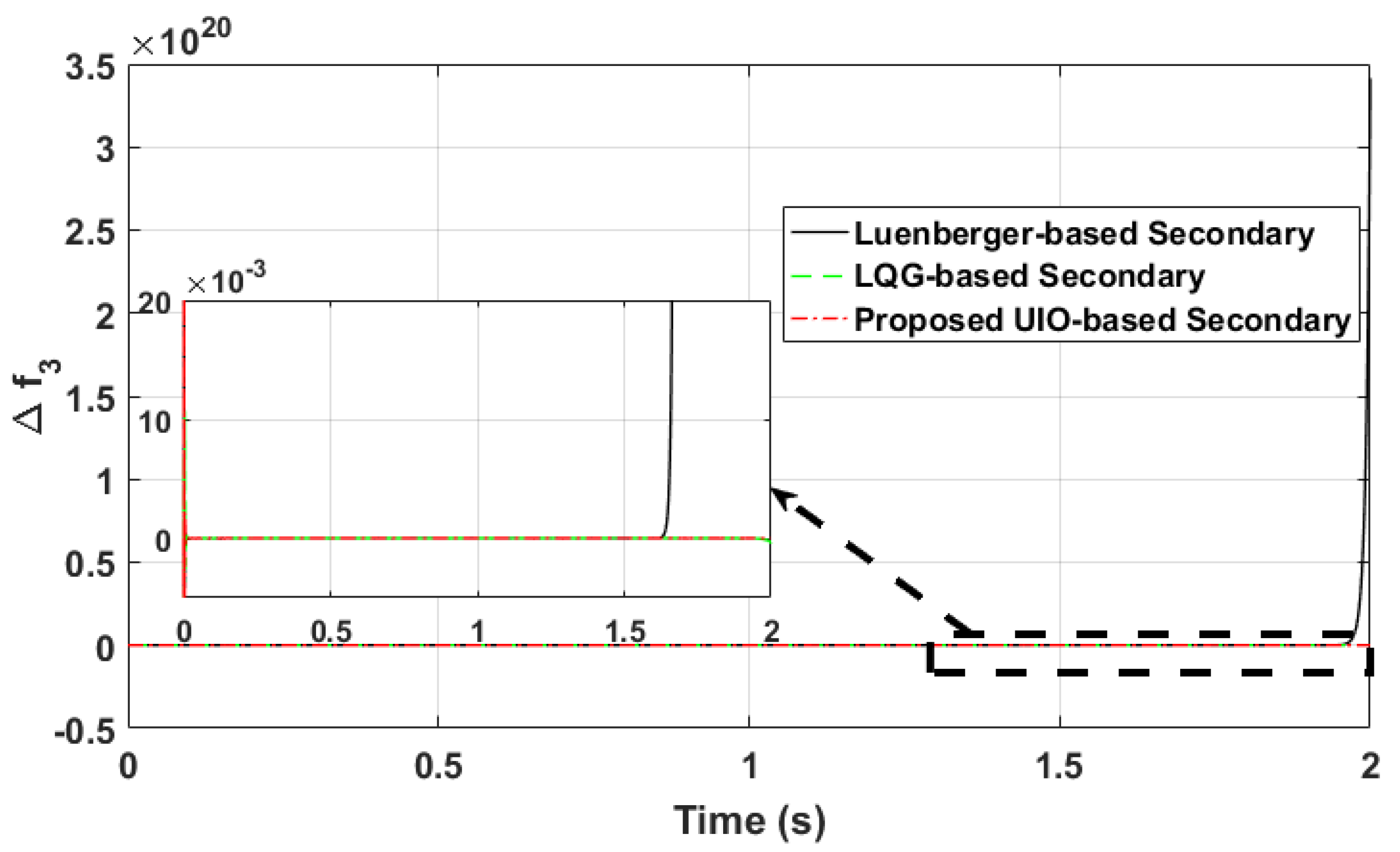
In this case, the stealthy FDI effect to one inverter angle is investigated. As seen in 10, all inverter angle dynamics are a function of the first inverter active power . Thus, one destructive FDI can be launched once is stealthily disclosed and used in the data injection. The FDI is added to the actuator of inverter angle 2 at s as:
The angles of inverters 2 and 3 for the microgrid with only primary control and with three secondary controllers are demonstrated in Figure 14 and Figure 15. Considering the results, the proposed UIO controller can still resiliently control the microgrid; however, this stealthy FDI can destabilize the microgrid equipped with LQG and Luenberger-based secondary control. The Luenberger-based secondary controller operates significantly more unstable compared to the LQG-based controller. Also, the inverters’ frequencies shown in Figure 16 and Figure 17 prove that the proposed UIO controller, unlike the other secondary controllers, compensates the inverters’ frequencies. In fact, this simulation case verifies that the proposed UIO-based controller properly maintains the microgrid resiliency.
6. Conclusions
This paper shows a procedure to develop a secondary control for an islanded microgrid. This islanded microgrid model includes inverter-based energy resources. To design a secure microgrid, the secondary control needs to operate resiliently against cyber anomalies, e.g., False Data Injection (FDI). In this paper, we show that the inverter-based microgrid can be tremendously vulnerable to stealthy FDI, and this type of cyber-disruption can make the microgrid unstable. We develop a secondary control based on Unknown Input Observer (UIO) and optimal compensator to regulate frequency of an islanded microgrid. The proposed secondary control can be effective against different types of FDIs.
Author Contributions
Methodology, M.R.K.; Writing, M.R.K., S.K.S. and J.M.S.; Validation, M.R.K., V.V. All authors have read and agreed to the published version of the manuscript.
Funding
Partial support of this research was provided by the Woodrow W. Everett, Jr. SCEEE Development Fund in cooperation with the Southeastern Association of Electrical Engineering Department Heads and National Science Foundation’s Division Of Electrical, Communication & Cyber System Grant # 1351201. Any opinions, findings, and conclusions, or recommendations expressed in this material are those of the author(s) and do not necessarily reflect the views of the sponsoring agency.
Conflicts of Interest
The authors declare no conflict of interest.
References
- Khalghani, M.R.; Solanki, J.; Solanki, S.K.; Khooban, M.H.; Sargolzaei, A. Resilient Frequency Control Design for Microgrids Under False Data Injection. IEEE Trans. Ind. Electron. 2021, 68, 2151–2162. [Google Scholar] [CrossRef]
- Khalghani, M.R.; Solanki, J.; Khushalani-Solanki, S.; Sargolzaei, A. Stochastic Load Frequency Control of Microgrids Including Wind Source Based on Identification Method. In Proceedings of the 2018 IEEE International Conference on Environment and Electrical Engineering and 2018 IEEE Industrial and Commercial Power Systems Europe (EEEIC/I CPS Europe), Palermo, Italy, 12–15 June 2018; pp. 1–6. [Google Scholar] [CrossRef]
- Victorio, M.; Sargolzaei, A.; Khalghani, M.R. A Secure Control Design for Networked Control Systems with Linear Dynamics under a Time-Delay Switch Attack. Electronics 2021, 10, 322. [Google Scholar] [CrossRef]
- Khalghani, M.R.; Solanki, J.; Solanki, S.K.; Sargolzaei, A. Resilient and Stochastic Load Frequency Control of Microgrids. In Proceedings of the 2019 IEEE Power Energy Society General Meeting (PESGM), Atlanta, GA, USA, 4–8 August 2019; pp. 1–5. [Google Scholar] [CrossRef]
- Qi, J.; Hahn, A.; Lu, X.; Wang, J.; Liu, C.C. Cybersecurity For Distributed Energy Resources And Smart Inverters. IET Cyber-Phys. Syst. Theory Appl. 2016, 1, 28–39. [Google Scholar] [CrossRef] [Green Version]
- Bidram, A.; Poudel, B.; Damodaran, L.; Fierro, R.; Guerrero, J.M. Resilient and Cybersecure Distributed Control of Inverter-Based Islanded Microgrids. IEEE Trans. Ind. Inform. 2020, 16, 3881–3894. [Google Scholar] [CrossRef]
- Nguyen, T.L.; Tran, Q.T.; Caire, R.; Gavriluta, C.; Nguyen, V.H. Agent Based Distributed Control Of Islanded Microgrid—Real-Time Cyber-Physical Implementation. In Proceedings of the 2017 IEEE PES Innovative Smart Grid Technologies Conference Europe (ISGT-Europe), Turin, Italy, 26–29 September 2017; pp. 1–6. [Google Scholar] [CrossRef] [Green Version]
- Zhou, Q.; Shahidehpour, M.; Alabdulwahab, A.; Abusorrah, A. A Cyber-Attack Resilient Distributed Control Strategy In Islanded Microgrids. IEEE Trans. Smart Grid 2020, 11, 3690–3701. [Google Scholar] [CrossRef]
- Mahmud, R.; Seo, G.S. Blockchain-Enabled Cyber-Secure Microgrid Control Using Consensus Algorithm. In Proceedings of the 2021 IEEE 22nd Workshop on Control and Modelling of Power Electronics (COMPEL), Cartagena, Colombia, 2–5 November 2021; pp. 1–7. [Google Scholar] [CrossRef]
- Zografopoulos, I.; Konstantinou, C. Detection of Malicious Attacks In Autonomous Cyber-Physical Inverter-Based Microgrids. IEEE Trans. Ind. Inform. 2021, 1. [Google Scholar] [CrossRef]
- Liu, S.; Hu, Z.; Wang, X.; Wu, L. Stochastic Stability Analysis and Control of Secondary Frequency Regulation for Islanded Microgrids Under Random Denial of Service Attacks. IEEE Trans. Ind. Inform. 2019, 15, 4066–4075. [Google Scholar] [CrossRef]
- Lu, L.Y.; Liu, H.J.; Zhu, H.; Chu, C.C. Intrusion Detection in Distributed Frequency Control of Isolated Microgrids. IEEE Trans. Smart Grid 2019, 10, 6502–6515. [Google Scholar] [CrossRef]
- Nguyen, T.L.; Wang, Y.; Tran, Q.T.; Caire, R.; Xu, Y.; Besanger, Y. Agent-based Distributed Event-Triggered Secondary Control for Energy Storage System in Islanded Microgrids-Cyber-Physical Validation. In Proceedings of the 2019 IEEE International Conference on Environment and Electrical Engineering and 2019 IEEE Industrial and Commercial Power Systems Europe (EEEIC/I CPS Europe), Genova, Italy, 11–14 June 2019; pp. 1–6. [Google Scholar] [CrossRef]
- Pogaku, N.; Prodanovic, M.; Green, T.C. Modeling, Analysis and Testing of Autonomous Operation of an Inverter-Based Microgrid. IEEE Trans. Power Electron. 2007, 22, 613–625. [Google Scholar]
- Banadaki, A.D.; Mohammadi, F.D.; Feliachi, A. State Space Modeling of Inverter Based Microgrids Considering Distributed Secondary Voltage Control. In Proceedings of the 2017 North American Power Symposium (NAPS), Morgantown, WV, USA, 17–19 September 2017; pp. 1–6. [Google Scholar]
- Banadaki, A.D.; Feliachi, A.; Kulathumani, V.K. Fully Distributed Secondary Voltage Control in Inverter-Based Microgrids. In Proceedings of the 2018 IEEE/PES Transmission and Distribution Conference and Exposition (T&D), Denver, CO, USA, 16–19 April 2018; pp. 1–9. [Google Scholar]
- Keshtkar, H.; Mohammadi, F.D.; Solanki, J.; Solanki, S.K. Multi-Agent Based Control of a Microgrid Power System in Case of Cyber Intrusions. In Proceedings of the 2020 IEEE Kansas Power and Energy Conference (KPEC), Manhattan, KS, USA, 13–14 July 2020; pp. 1–6. [Google Scholar] [CrossRef]
- Rasheduzzaman, M.; Mueller, J.A.; Kimball, J.W. Reduced-Order Small-Signal Model of Microgrid Systems. IEEE Trans. Sustain. Energy 2015, 6, 1292–1305. [Google Scholar] [CrossRef]
- Khalghani, M.R.; Khushalani-Solanki, S.; Solanki, J.; Sargolzaei, A. Cyber Disruption Detection In Linear Power Systems. In Proceedings of the 2017 North American Power Symposium (NAPS), Morgantown, WV, USA, 17–19 September 2017; pp. 1–6. [Google Scholar]
- Hou, M.; Muller, P.C. Design of Observers for Linear Systems with Unknown Inputs. IEEE Trans. Autom. Control. 1992, 37, 871–875. [Google Scholar] [CrossRef]
- Guo, F.; Wen, C.; Mao, J.; Song, Y.D. Distributed Secondary Voltage and Frequency Restoration Control of Droop-Controlled Inverter-Based Microgrids. IEEE Trans. Ind. Electron. 2015, 62, 4355–4364. [Google Scholar] [CrossRef]
- Liu, C.; Deng, R.; He, W.; Liang, H.; Du, W. Optimal Coding Schemes for Detecting False Data Injection Attacks in Power System State Estimation. IEEE Trans. Smart Grid 2022, 13, 738–749. [Google Scholar] [CrossRef]
Figure 1.
General diagram of DG inverter connected to Microgrids [14].
Figure 1.
General diagram of DG inverter connected to Microgrids [14].

Figure 2.
External power controller diagram of DG inverter [14].
Figure 2.
External power controller diagram of DG inverter [14].

Figure 3.
Network topology of inverter-based microgrid model [14].
Figure 3.
Network topology of inverter-based microgrid model [14].
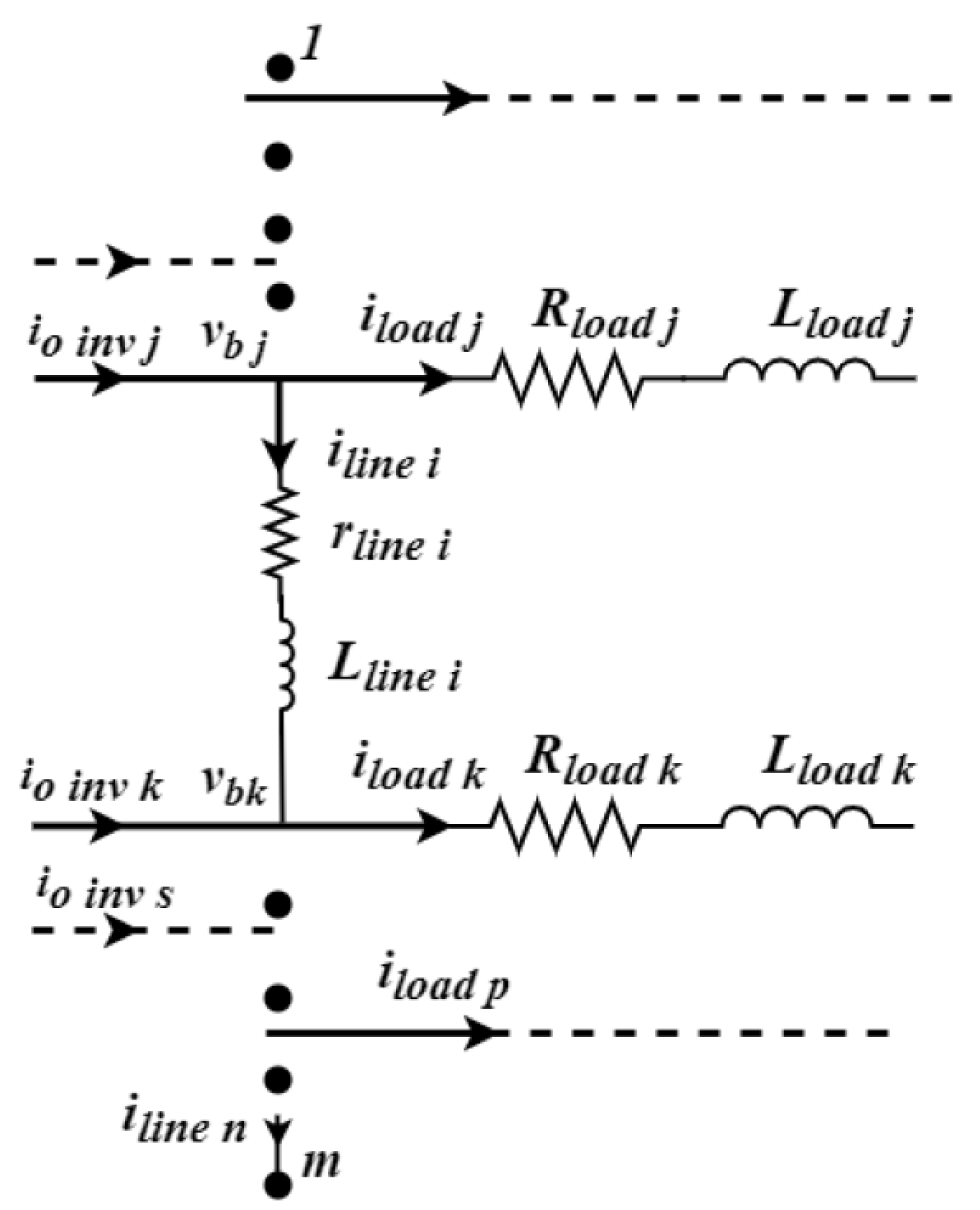
Figure 4.
The proposed control strategy for islanded microgrid.
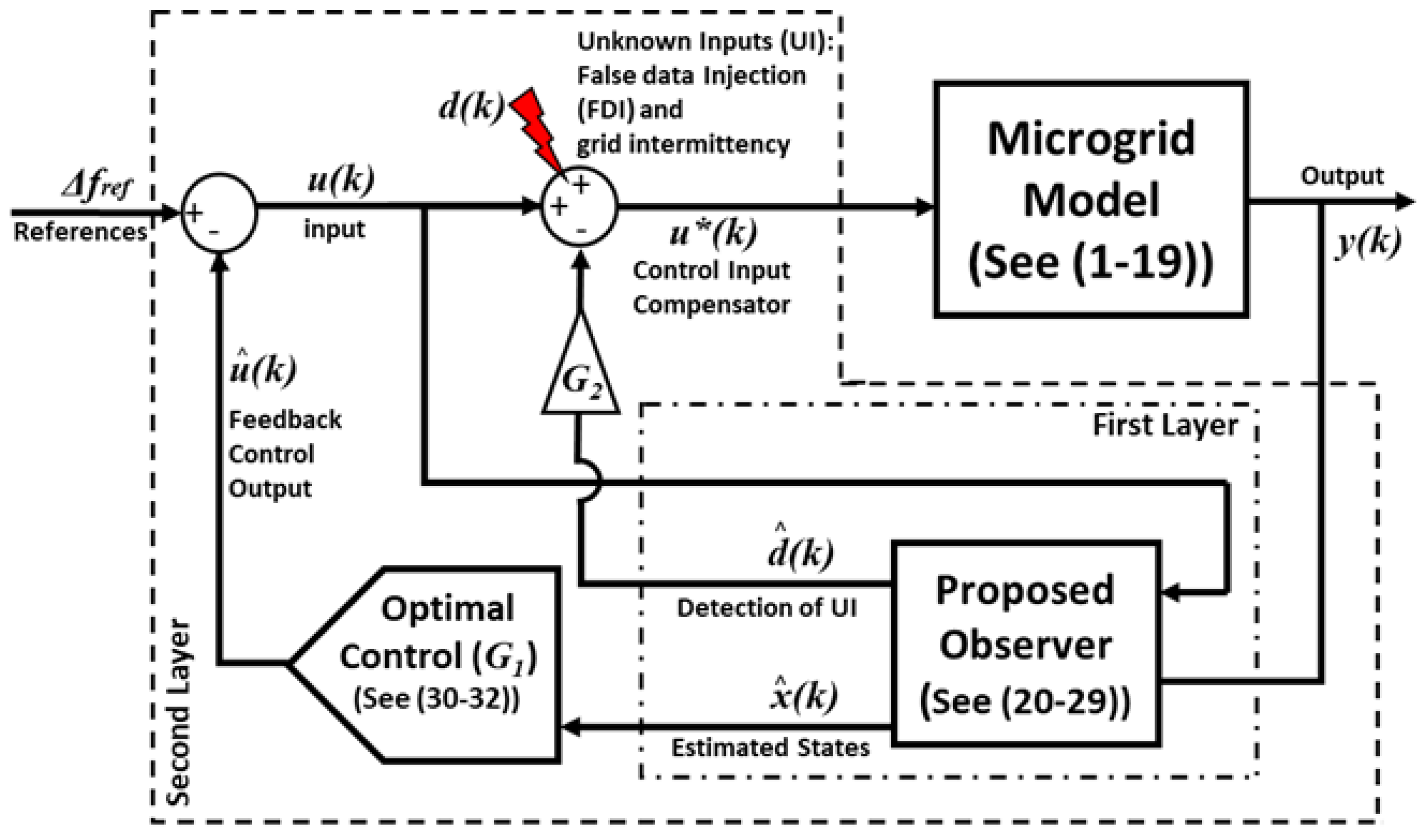
Figure 5.
Case study: microgrid topology.
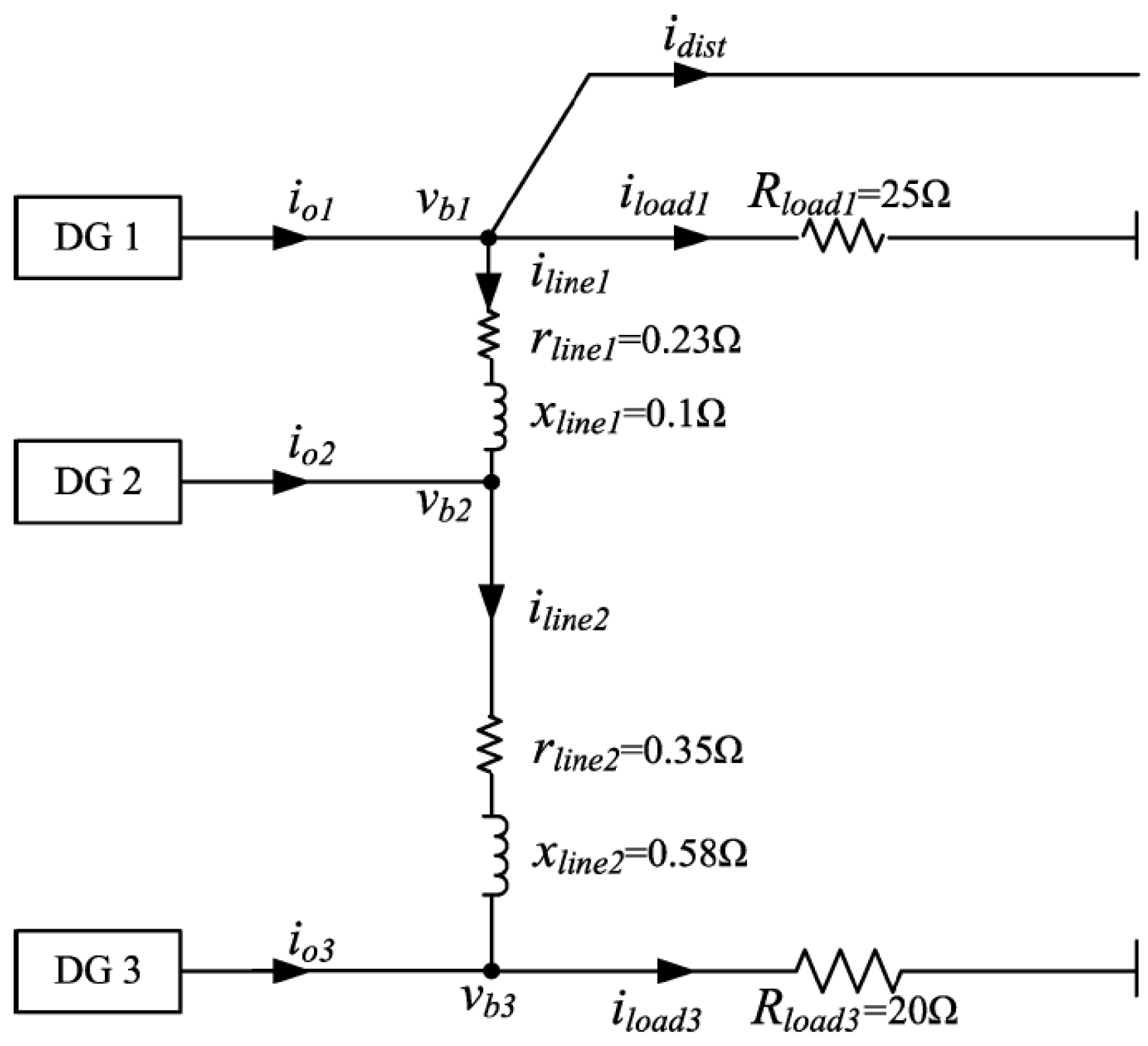
Figure 6.
Second inverter angle in scenario 1 (Step load change).
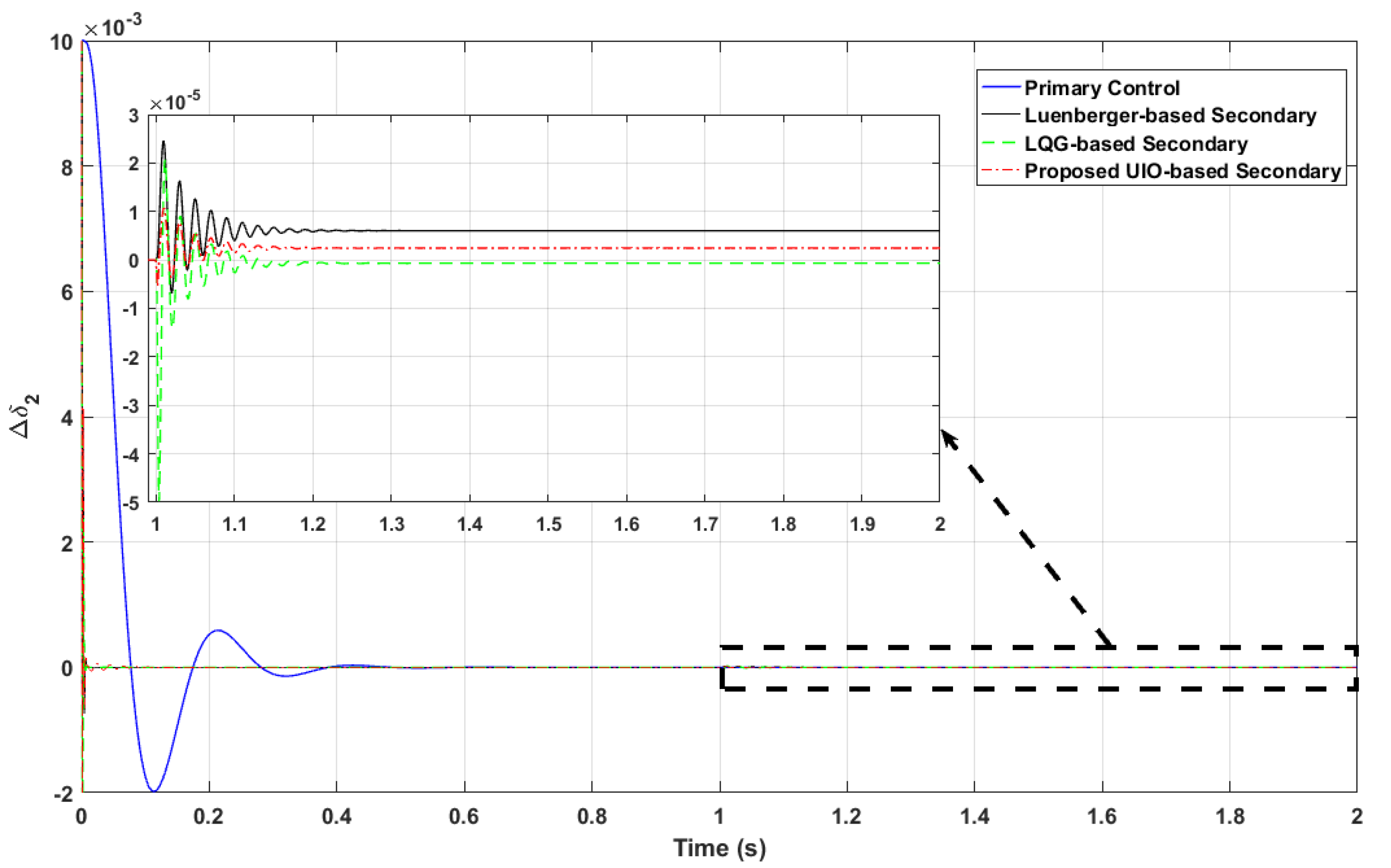
Figure 7.
Third inverter angle in scenario 1 (Step load change).
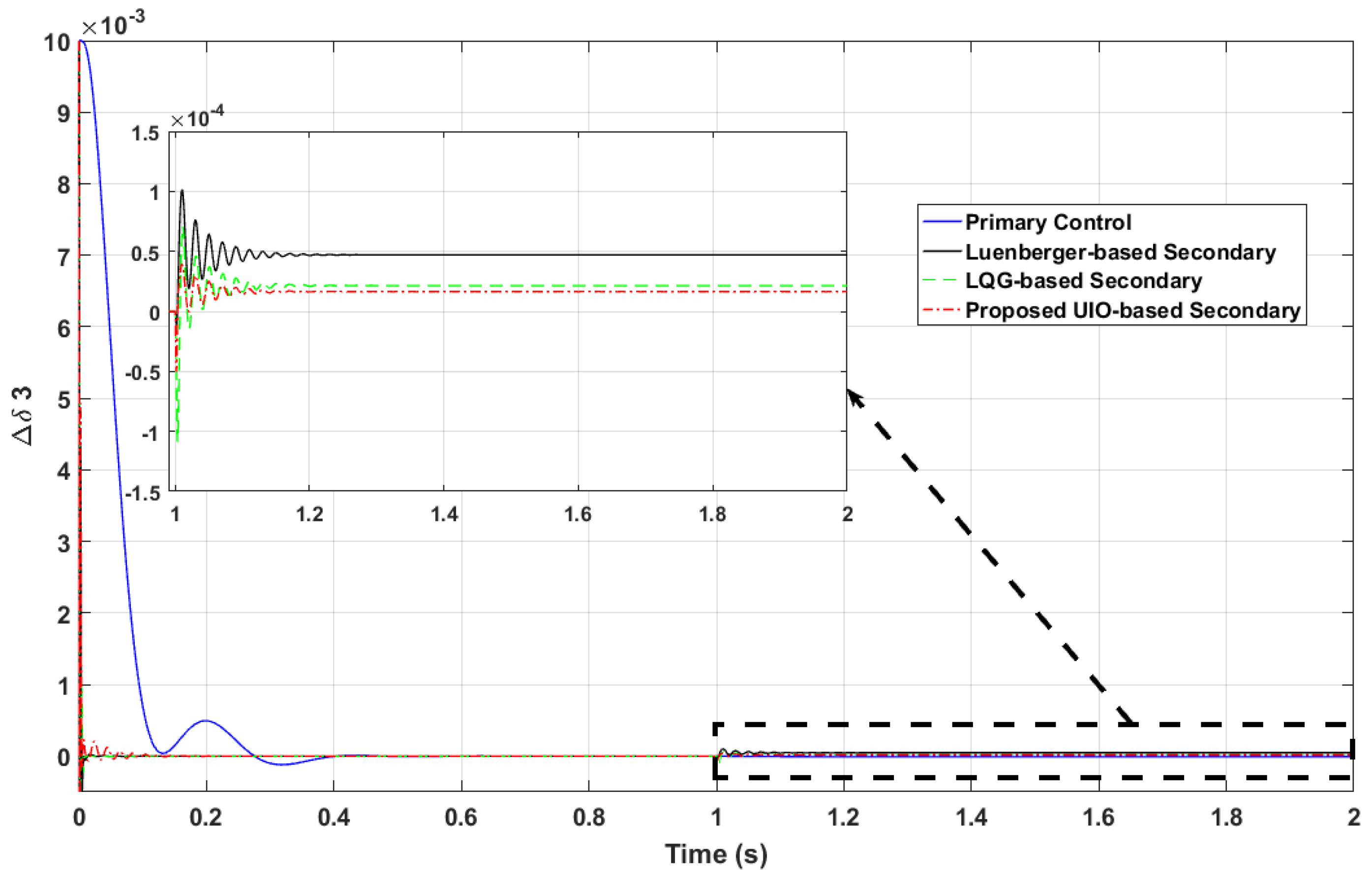
Figure 8.
Second inverter frequency dynamic in scenario 1 (Step load change).
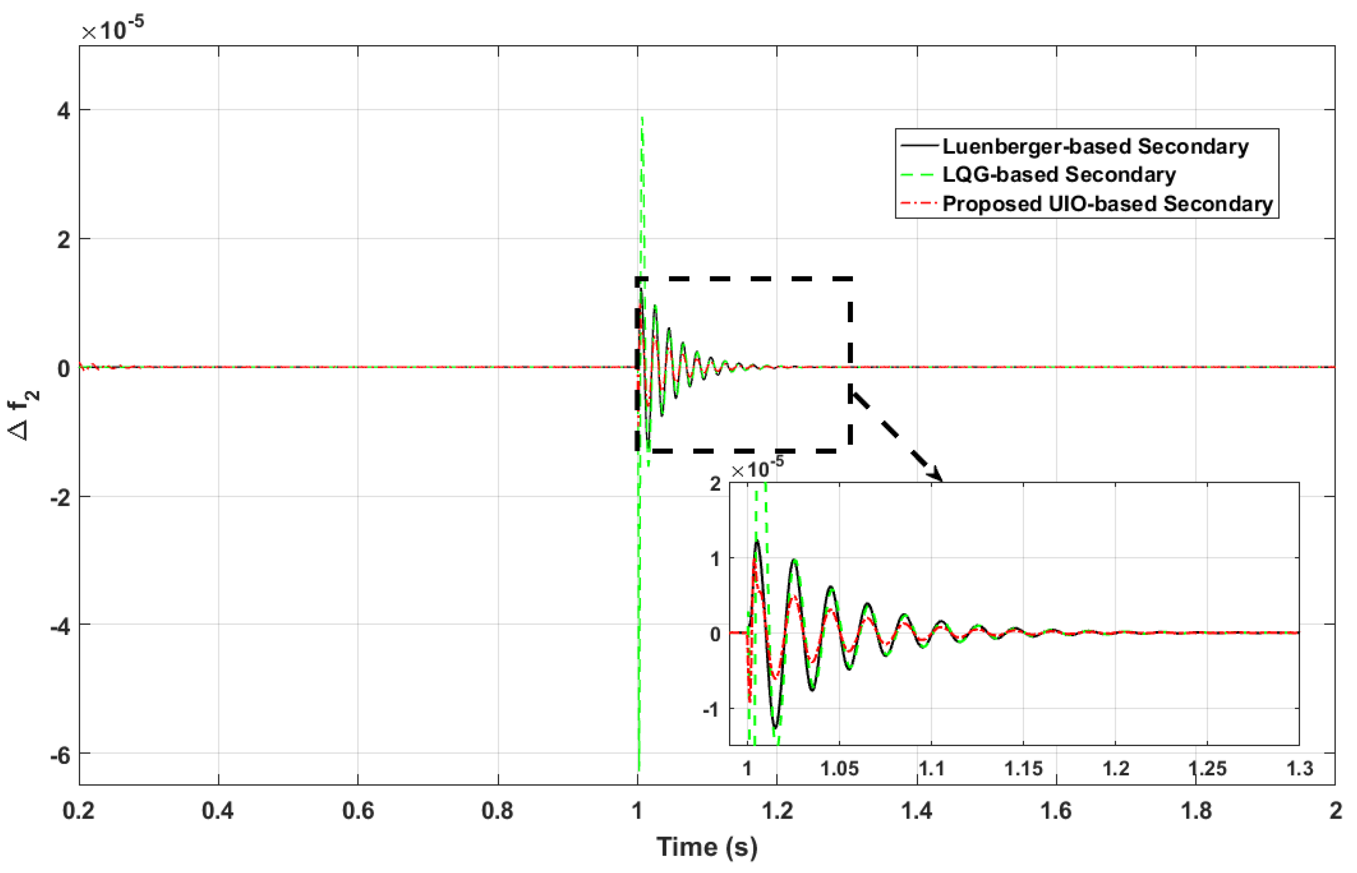
Figure 9.
Third inverter frequency dynamic in scenario 1 (Step load change).

Figure 10.
Second inverter angle in scenario 2 (False Data Injection (FDI) into second inverter’s actuator).
Figure 10.
Second inverter angle in scenario 2 (False Data Injection (FDI) into second inverter’s actuator).

Figure 11.
Third inverter angle in scenario 2 (FDI into second inverter’s actuator).
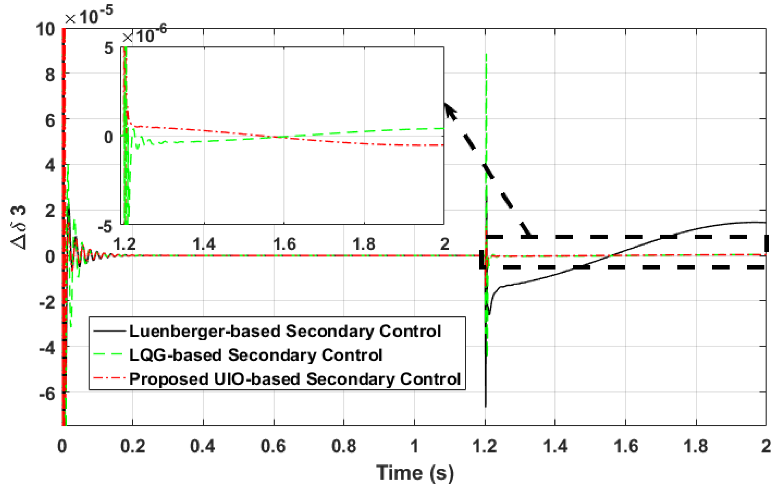
Figure 12.
Second inverter frequency dynamic in scenario 2 (FDI into second inverter’s actuator).
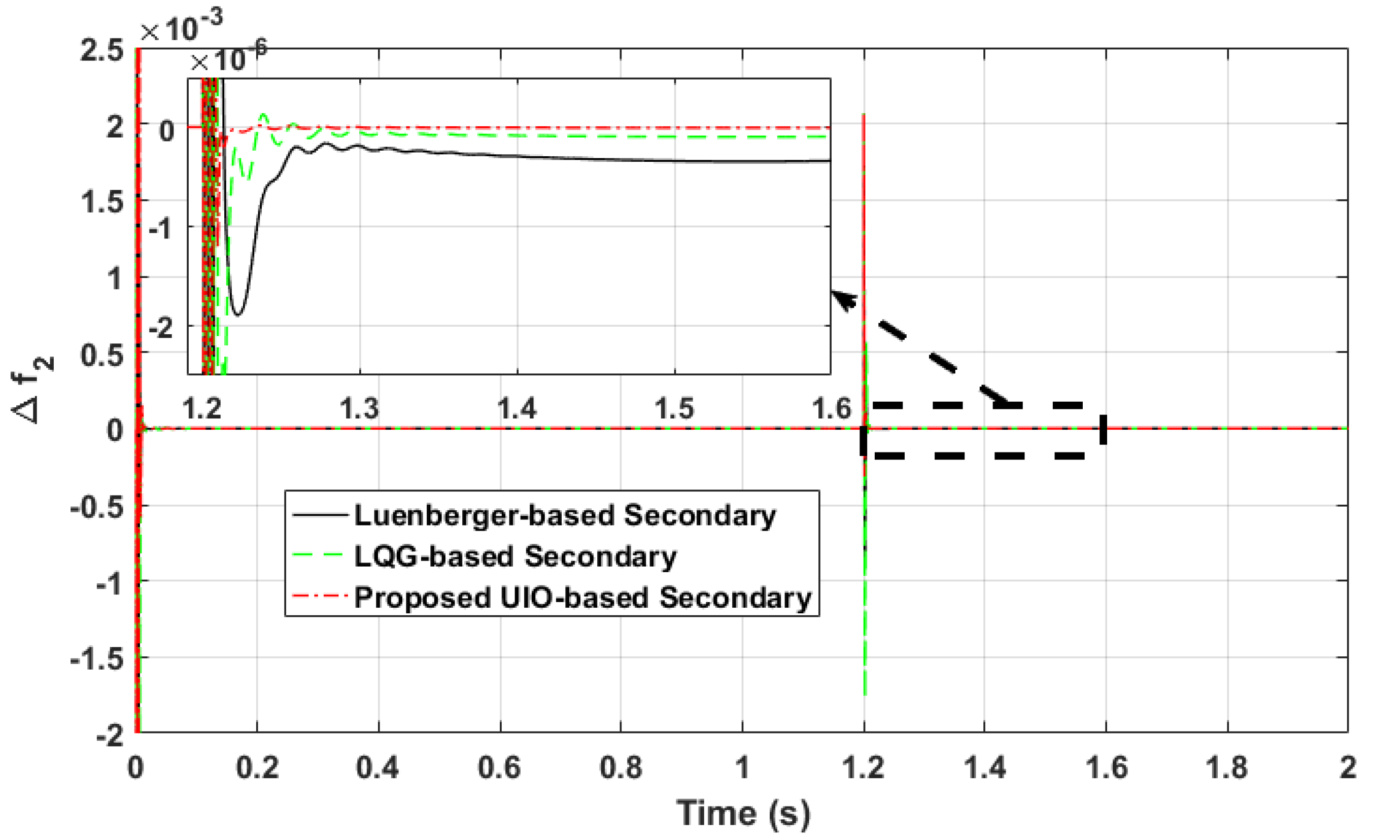
Figure 13.
Third inverter frequency dynamic in scenario 2 (FDI into second inverter’s actuator).

Figure 14.
Second inverter angle in scenario 3 (Stealthy FDI to second inverter’s actuator).
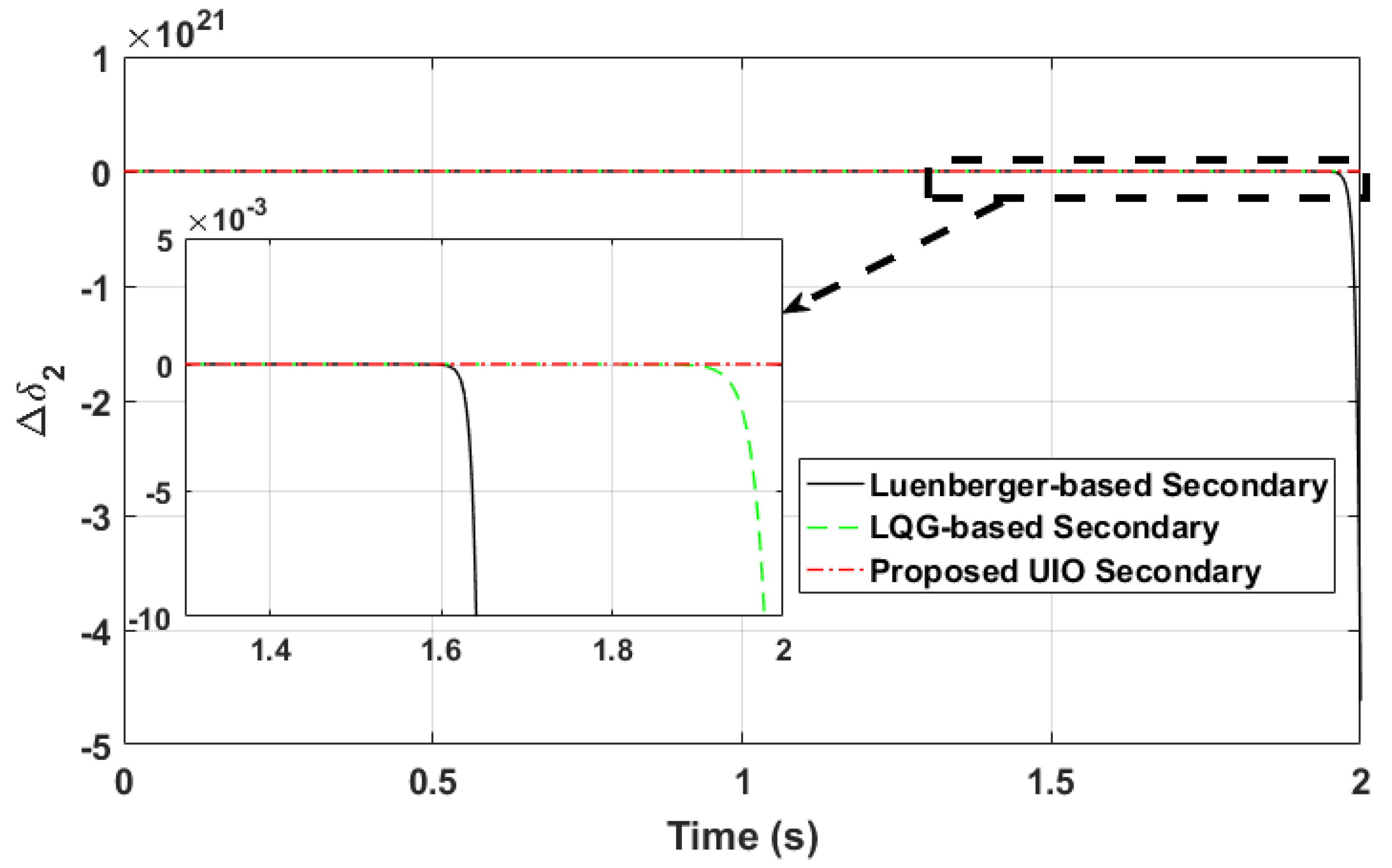
Figure 15.
Third inverter angle in scenario 3 (Stealthy FDI to second inverter’s actuator).

Figure 16.
Second inverter frequency dynamic in scenario 3 (Stealthy FDI to second inverter’s actuator).
Figure 16.
Second inverter frequency dynamic in scenario 3 (Stealthy FDI to second inverter’s actuator).
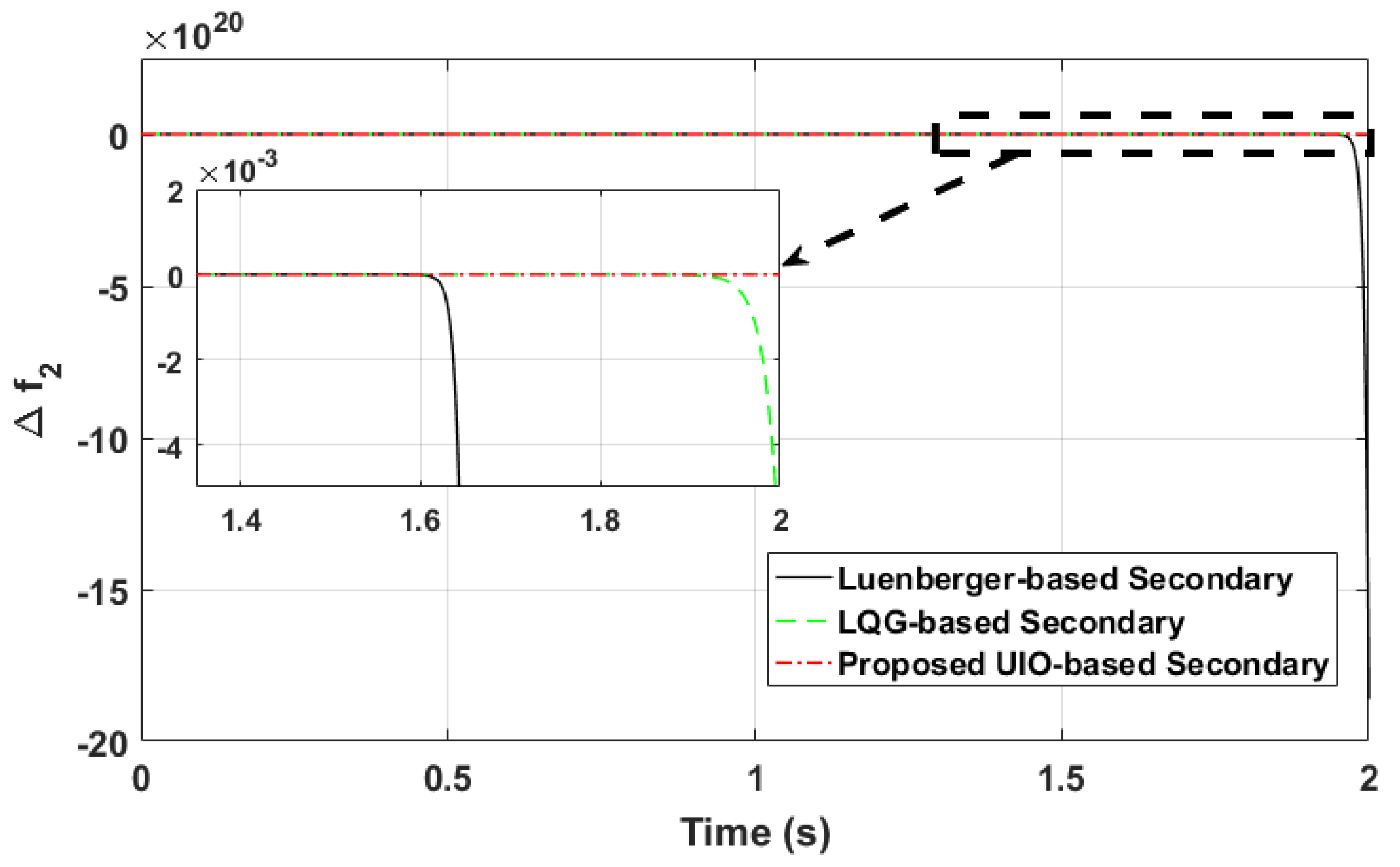
Figure 17.
Third inverter frequency dynamic in scenario 3 (Stealthy FDI to second inverter’s actuator).
Figure 17.
Third inverter frequency dynamic in scenario 3 (Stealthy FDI to second inverter’s actuator).

Table 1.
Eigenvalues of the microgrid (A matrix).
| Standard Inverter-Based Microgrid Model | Reduced-Order Inverter- Based Microgrid Model | |
|---|---|---|
| Eigenvalues | −9.44e6 + j3.14e2 | −9.44e6 + j3.14e2 |
| −9.44e6 − j3.14e2 | −9.44e6 − j3.14e2 | |
| −3.63e6 + j3.14e2 | −3.63e6 + j3.14e2 | |
| −3.63e6 − j3.14e2 | −3.63e6 − j3.14e2 | |
| −2.85e6 + j3.14e2 | −2.85e6 + j3.14e2 | |
| −2.85e6 − j3.14e2 | −2.85e6 − j3.14e2 | |
| −2.94e3 + j7.38e3 | −2.94e3 + j7.38e3 | |
| −2.94e3 − j7.38e3 | −2.94e3 − j7.38e3 | |
| −2.79e3 + j6.84e3 | −2.79e3 + j6.84e3 | |
| −2.79e3 − j6.84e3 | −2.79e3 − j6.84e3 | |
| −2.84e3 + j4.89e3 | −2.84e3 + j4.89e3 | |
| −2.84e3 − j4.89e3 | −2.84e3 − j4.89e3 | |
| −2.53e3 + j4.43e3 | −2.53e3 + j4.43e3 | |
| −2.53e3 − j4.43e3 | −2.53e3 − j4.43e3 | |
| −2.86e3 + j2.92e3 | −2.86e3 + j2.92e3 | |
| −2.86e3 − j2.92e3 | −2.86e3 − j2.92e3 | |
| −2.21e3 + j2.20e3 | −2.21e3 + j2.20e3 | |
| −2.21e3 − j2.20e3 | −2.21e3 − j2.20e3 | |
| −1.49e3 + j2.51e3 | −1.49e3 + j2.51e3 | |
| −1.49e3 − j2.51e3 | −1.49e3 − j2.51e3 | |
| −1.29e3 + j2.10e3 | −1.29e3 + j2.10e3 | |
| −1.29e3 − j2.10e3 | −1.29e3 − j2.10e3 | |
| −1.31e3 + j1.71e3 | −1.31e3 + j1.71e3 | |
| −1.31e3 − j1.71e3 | −1.31e3 − j1.71e3 | |
| −1.22e3 + j1.65e3 | −1.22e3 + j1.65e3 | |
| −1.22e3 − j1.65e3 | −1.22e3 − j1.65e3 | |
| −1.14e3 + j1.54e3 | −1.14e3 + j1.54e3 | |
| −1.14e3 − j1.54e3 | −1.14e3 − j1.54e3 | |
| −1.11e3 + j1.50e3 | −1.11e3 + j1.50e3 | |
| −1.11e3 − j1.50e3 | −1.11e3 − j1.50e3 | |
| −2.00e1 + j3.13e2 | −2.00e1 + j3.13e2 | |
| −2.00e1 − j3.13e2 | −2.00e1 − j3.13e2 | |
| −2.50e1 + j3.13e2 | −2.50e1 + j3.13e2 | |
| −2.50e1 − j3.13e2 | −2.50e1 − j3.13e2 | |
| −1.42e2 + j2.10e2 | −1.42e2 + j2.10e2 | |
| −1.42e2 − j2.10e2 | −1.42e2 − j2.10e2 | |
| −1.23e2 + j1.50e2 | −1.23e2 + j1.50e2 | |
| −1.23e2 − j1.50e2 | −1.23e2 − j1.50e2 | |
| −13.48 + j30.21 | −13.48 + j30.21 | |
| −13.48 − j30.21 | −13.48 − j30.21 | |
| −15.53 + j10.59 | −15.53 + j10.59 | |
| −15.53 − j10.59 | −15.53 − j10.59 | |
| −20.84 | −20.84 | |
| −28.25 | −28.25 | |
| −31.38 | −31.38 | |
| −31.40 | −31.40 | |
| 0 | Removed |
Table 2.
Microgrid parameters.
| Inverter Parameters | |||
|---|---|---|---|
| Parameter | Value | Parameter | Value |
| 8 kHz | 9.4 | ||
| 1.35 mH | |||
| 50 F | 0.05 | ||
| 0.1 Ohm | 390 | ||
| 0.35 mH | 10.5 | ||
| 0.03 Ohm | |||
| 31.41 | F | 0.75 | |
Table 3.
Microgrid initial conditions.
| Initial Conditions | |||
|---|---|---|---|
| Parameter | Value | Parameter | Value |
| [380.8 381.8 380.4] | [0 0 0] | ||
| [11.4 11.4 11.4] | [0.4 −1.45 1.25] | ||
| [11.4 11.4 11.4] | [−5.5 −7.3 −4.6] | ||
| [379.5 380.5 379] | [−6 −6 −5] | ||
| [314] | [0 1.9 −3 −0.0113] | ||
| [−3.8] | [0.4] | ||
| [7.6] | [−1.3] | ||
Publisher’s Note: MDPI stays neutral with regard to jurisdictional claims in published maps and institutional affiliations. |
© 2022 by the authors. Licensee MDPI, Basel, Switzerland. This article is an open access article distributed under the terms and conditions of the Creative Commons Attribution (CC BY) license (https://creativecommons.org/licenses/by/4.0/).
Share and Cite
MDPI and ACS Style
Khalghani, M.R.; Verma, V.; Khushalani Solanki, S.; Solanki, J.M. Resilient Networked Control of Inverter-Based Microgrids against False Data Injections. Electronics 2022, 11, 780. https://doi.org/10.3390/electronics11050780
AMA Style
Khalghani MR, Verma V, Khushalani Solanki S, Solanki JM. Resilient Networked Control of Inverter-Based Microgrids against False Data Injections. Electronics. 2022; 11(5):780. https://doi.org/10.3390/electronics11050780
Chicago/Turabian StyleKhalghani, Mohammad Reza, Vishal Verma, Sarika Khushalani Solanki, and Jignesh M. Solanki. 2022. "Resilient Networked Control of Inverter-Based Microgrids against False Data Injections" Electronics 11, no. 5: 780. https://doi.org/10.3390/electronics11050780
Note that from the first issue of 2016, this journal uses article numbers instead of page numbers. See further details here.