
An Improved Image Enhancement Method for Traffic Sign Detection

Department of IT Systems and Networks, University of Debrecen, H-4028 Debrecen, Hungary
Electronics 2022, 11(6), 871; https://doi.org/10.3390/electronics11060871
Submission received: 1 February 2022
/
Revised: 7 March 2022
/
Accepted: 7 March 2022
/
Published: 10 March 2022
(This article belongs to the Special Issue AI for Embedded Systems)
Abstract
:Traffic sign detection (TRD) is an essential component of advanced driver-assistance systems and an important part of autonomous vehicles, where the goal is to localize image regions that contain traffic signs. Over the last decade, the amount of research on traffic sign detection and recognition has significantly increased. Although TRD is a built-in feature in modern cars and several methods have been proposed, it is a challenging problem due to the high computational demand, the large number of traffic signs, complex traffic scenes, and occlusions. In addition, it is not clear how can we perform real-time traffic sign detection in embedded systems. In this paper, we focus on image enhancement, which is the first step of many object detection methods. We propose an improved probability-model-based image enhancement method for traffic sign detection. To demonstrate the efficiency of the proposed method, we compared it with other widely used image enhancement approaches in traffic sign detection. The experimental results show that our method increases the performance of object detection. In combination with the Selective Search object proposal algorithm, the average detection accuracies were 98.64% and 99.1% on the GTSDB and Swedish Traffic Signs datasets. In addition, its relatively low computational cost allows for its usage in embedded systems.
1. Introduction
In recent years, traffic scene analysis has become a hot topic due to the large investment into autonomous vehicles and advanced driver-assistance systems. Two of its key components are traffic sign detection (TSD) and recognition (TSR). TSD is the process of localizing signs on an input image. In other worlds, TSD methods generate candidate regions of interest (ROIs) that are likely to contain traffic signs. Then, the detected image regions are used to feed the traffic sign recognizer (or classifier), which tries to identify the exact type of sign. Therefore, the efficiency of sign detection has a huge impact on the output of the whole sign recognition process.
TSD is still a challenging problem. Although the industrial and academic research community has achieved remarkable results in TSD, it is not a fully accomplished task yet. The difficulty comes from complex traffic scenes, including weather conditions, variable illumination, environmental noise, sign color fading, etc.
The information content of road signs is coded into their visual appearance. They are designed to be unique and to have distinguishable features, such as color and shape. In order to standardize traffic signs in different countries, an international agreement (Vienna Convention of Road Signs and Signals) was accepted in 1968. The agreement was signed by 52 countries, of which 31 are European countries [1]. The Vienna Convention classified road signs into eight categories, such as danger, priority, mandatory, etc.
Typically, signs have a simple shape and eye-catching color. For example, the most common colors of European traffic signs are red and blue. These features are the basis of several earlier published TSD methods [2]. However, color and shape features are vulnerable for various reasons. The original color slightly changes due to damage over the years or moving cameras. In addition, color perception is sensitive to other factors, such as distance from the sign, reflection, time of day, and weather conditions. Such effects make the image segmentation process hard.
In order to overcome these difficulties, researchers have used different image enhancement techniques to suppress backgrounds and highlight traffic signs on images. In some cases, image enhancement is based on color-channel thresholding in the RGB (red, green, and blue channels) or other color spaces, such as HSI (hue, saturation, and intensity channels) [3]. In this case, the efficiency of image enhancement strongly depends on a set of thresholds defined by the researcher. In other cases, researchers have used color-channel normalization or even machine learning methods for image enhancement. Since we have more choices for image enhancement, a question may arise: which of these methods are the most efficient?
In this paper, we are focus on image enhancement and propose an improved probability-model-based method. Its efficiency was tested in the traffic sign detection problem. The purpose of this method is to reject uninteresting regions (background) and keep the original traffic sign shape. Our experimental results show that the proposed image enhancement method improves the performance of an object detector.
2. Public Traffic Sign Detection Benchmarks
Freely available traffic sign detection databases provide information sources for TSD system development. Some databases contain multimodal data acquired from different types of sensors [4], but most of them include only road scene images. Such databases can be used not just as data sources but also as benchmarks. All of them contain annotated (labelled) images about driving scenes, which can be used to train and test detector models. In recent years, most TSD algorithms have been developed with public databases because doing so allows for objective comparison of TSD methods. As a data source, we used two popular databases, namely the German Traffic Sign Detection Benchmark (GTSDB) and the Swedish Traffic Signs database.
The GTSDB, made for a 2013 competition, is the most popular database on this topic [5]. It was one of the first benchmarks of the traffic sign detection problem. The dataset consists of natural traffic scenes captured during daytime and at night under different weather conditions. It includes 900 images (stored in ppm format), which contain 1206 traffic signs. Out of the 900 images, 600 images constitute the training set, whereas the remaining 300 images are the test set. All images have a 1360 × 800 pixel resolution with zero to six traffic signs varying in size between 16 × 16 and 128 × 128 pixels. The database and additional information about it are available on the official website: https://benchmark.ini.rub.de/gtsdb_dataset.html (accessed on 13 November 2021).
The Swedish Traffic Signs dataset was captured on Swedish highways and city roads [6]. The image-capture device was a 1.3 megapixel color camera located on a car’s dashboard. The whole dataset consists of 20,000 images, but only 20% of them are labelled. The labelled part is divided into two sets. In this work, we used the second set as our test data. A detailed description of the Swedish Traffic Signs dataset can be found at https://www.cvl.isy.liu.se/research/datasets/traffic-signs-dataset/ (accessed on 24 February 2022).
3. Related Work
In recent years, a large number of TSD approaches based on machine learning and machine vision have been published. These approaches can be classified according to the used region (or object) proposal algorithm. Several earlier methods use the sliding-window approach, where a fixed-size “window” goes through horizontally and vertically on different scaled versions of an image. For example, Wang et al. [7] used this region proposal technique twice (coarse and fine filtering) to detect candidate image regions where signs could be located. In the coarse-filtering step, the window size was 20 × 20 pixels, whereas in the fine-filtering step, it was 40 × 40 pixels. Both steps were performed 22 times on downscaled images with a scaling factor of 1.1.
In most sliding-window-based object localization approaches, the authors have not used image enhancement; therefore, features have been extracted from the original image regions. Although the sliding-window approach has high precision if both the window and the step size are relatively low, its time requirement is high as a result of the huge amount of image patches that need to be analyzed. As an example, a sliding window with a 1.1 scale factor, 5 pixel step size, and 20 × 20 kernel generates 242,748 image patches on a 1360 × 800 pixel image. Therefore, this is not the best option for real-time traffic sign detection in today’s embedded systems.
On the other hand, the researchers have combined image enhancement method(s) with shape matching, Maximum Stable Region (MSER), Selective Search, EdgeBox, or other types of object proposal algorithms to filter out traffic signs from the image.
Other researchers have applied color-channel thresholding for image enhancement. Berkaya et al. [8] applied different color thresholding for red and blue colors in the RGB color space. Some researchers converted RGB images into other color spaces because the RGB space is easily affected by lighting conditions. Yakimov [9] used three threshold values in the HSV color space to filter out the red color of traffic signs. Other researchers used thresholding in the HSI rather than the HSV color space [10]. Ellehyani et al. [11] defined different threshold values to the red and blue colors for all channels of the HSI space. In the below formulas, fh(x,y), fs(x,y), and fi(x,y) are the hue, saturation, and intensity values, respectively, of a pixel in the HSI color space, whereas f*(x,y) is the output image.
Another group of researchers think that simple thresholding is not effective and fixed threshold values may cause failure in the ROI extraction step. Therefore, they applied different color-channel normalization techniques in order to highlight the (typically red and blue) colors of traffic signs.
The authors of [12,13] tested RGB normalization. In addition to RGB normalization, Salti et al. [12] applied separated-channel normalization image enhancement approaches with and without color stretching. In (3) and (4), fr(x,y), fg(x,y), and fb(x,y) are the red, green, and blue intensities of a pixel.
Contrast stretching was applied to all channels of an RGB image to deal with under- or overexposure. In both cases, the RGB image was transformed into a single-channel image where the suitable channel (that characterizes the sought signal) was enhanced (e.g., blue in the case of mandatory signs). The authors concluded that in the case of red and white signs, color stretching is not necessary and both image enhancement techniques have the same efficiency. However, in the case of mandatory signs, channel normalization brought detection improvement. In their work, the enhanced image was the input for MSER segmentation. MSER can detect stable regions or blobs on gray-valued images wherein the distribution of pixel values has low variance.
The authors of [14,15] followed a similar approach as that used in [12], with an RB-channel-normalized image as the input for the MSER segmentation algorithm. Since blue and red are the two dominant background colors of traffic signs, Kurnianggoro et al. [15] tried to leave only the maximum value of those color channels (5).
Some researchers have used more complex approaches for image enhancement, with a shallow machine learning algorithm responsible for pixel categorization. Liang et al. [16] and Wu et al. [17] transformed an original RGB color image to a grayscale image with a Support Vector Machine (SVM). In their approach, positive colors (e.g., red in the danger category) are mapped to high intensities, and negative colors (e.g., all colors except red in the danger category) are mapped to low intensities. They categorized all colors as positive or negative (binary classification). The colors of the traffic signs belong to the positive category, labelled +1, whereas other colors belong to the negative category, labelled −1. In the case of prohibitory and danger signs, the red border pixels are treated as the positive color, whereas in the case of mandatory signs, the blue background pixels are treated as positive pixels. The binary training data generated in this way was used to train an SVM. After that, color pixel mapping was performed by the trained SVM according to (6), where frgb(x,y) is the red, green, and blue intensities; and f*(x,y) is the gray intensity of a pixel at coordinate (x,y).
This image enhancement method helped to them in the multiscale template matching process. Our image enhancement algorithm also requires such a training dataset, but its training and decision time is less than that of an SVM.
Beyond SVMs, other shallow machine learning methods are also used for pixel classification. For example, Ellahyani and Ansari [18] combined mean-shift (MS) clustering and random forest. MS is used as an image preprocessing step because the direct usage of random forest for all pixels would be a time-consuming process. Yang et al. [19,20] defined a probability model to compute the likelihood that a pixel falls into a particular color category. To construct the model, they manually collected training samples (pixel values) and converted them into the Ohta space. Their probability model is based on the Bayes rule, where the color class distribution is modelled by Gaussian distribution (7). In (7), foh(x,y) is the normalized components of a pixel (features) in the Ohta space, and μi and Σi are the mean vector and covariance matrix, respectively, of class Ci.
Our proposed approach is a similar naïve Bayes model. However, in spite of [19,20], we discretized all used features (color representation), and their distributions are modelled by their probability mass function. In addition, used features are selected according to their Kullback-Leibler (KL) divergence between classes.
A small group of researchers have focused only on specific traffic sign categories. For example, Wang et al. [21] and Gudigar et al. [22] proposed specific image enhancement methods for the detection of traffic signs with red rim. This condition covers prohibitory and danger signs. The authors of [21] converted RGB images into the HSV color space, where they exploited the color information of neighboring pixels. In the hue and saturation color planes, they determined the red degree of a color (fd(x,y)) with the following calculation:
Thereafter, for each pixel, they have taken a square window wx,y centered on fd(x,y) with radius Br and calculated the normalized red degree (fnd(x,y)) with the following formula:
where μ(wx,y) and σ(wx,y) are the mean and variance of the red degrees of all the pixels in wx,y. However, this method works only for a subset of traffic signs. Moreover, the window-wise calculation slows down the image enhancement process. In this article, we propose a generally usable image enhancement method.
4. Materials and Methods
In most images, the color of traffic signs is rather distinct from the background, making it an intuitive feature for traffic sign detection. In order to highlight traffic signs in images, we propose an improved probability model for image enhancement. Its task is to compute the likelihood that a pixel falls into one of the N classes, where one of them is the background.
The model requires a training set wherein image pixels are categorized into N classes. To test the efficiency of the model, 150 training images of the GTSDB and 100 images from the first labelled set of the Swedish Traffic Signs dataset were used as training data. All images were manually annotated with the Labelme software. Figure 1 shows such an annotated image with three classes (N = 3): red-colored traffic sign (c1), blue-colored traffic sign (c2), and background (c3). As can be seen in the image, rectangular regions were selected wherein all pixels belong to one of the three classes.
Before training, all of the collected pixels were converted from the RGB color space into other color representations for use as feature vectors. Formally, an frgb(x,y) pixel is represented with an fx,y vector, where fi is the i-th feature:
Our probability model is actually a naïve Bayes machine learning algorithm. It calculates the probability that the fx,y feature vector belongs to class ci with the Bayesian rule:
In the above formula, the probability of a feature vector (P(fx,y)) is a constant value in an image. Therefore, P(fx,y) can be eliminated. In addition, if we decompose vector elements, (11) can be rewritten as:
In (12), P(ci) is the prior class probability, whereas P(fk|ci) is the class-conditional density. The class-conditional density is approximated with the probability mass function of fk for ci. P(ci) can be easily computed from the number of samples in classes n(ci):
This model generates twice as many probability maps (matrices with the same dimension as the original image) as classes other than the background if we use different features in different classes. Since we used different features to separate red and blue colors from background (Section 5), we have four probability maps. The class probability maps are denoted with C0, C1, C2,0, C2,1, where C2,i is the background to class i. Those C values can be calculated by a simple algorithm shown in Algorithm 1. It is important to note that the above equations describe pixel-wise classification, whereas the algorithm below uses matrix operations in order to speed up the execution time.
| Algorithm 1: Get class probability map. |
| Require: Ensure: |
| … |
| … |
The elements of maps indicate the probability that a pixel at coordinate (x,y) belongs to class ci. Therefore, we need to keep only those probability values in C0 and C1 that are higher than the probability of background:
To construct the grayscale output image, we add the normalized forms of C*0 to C*1 and rescale the sum with the following formula, where ε is a very small number to avoid division by zero:
5. Results and Discussion
5.1. Feature Vector Construction
The above-described probability model works properly if “good” features are used for the representation of a color pixel. In order to find appropriate features, we tested the color channels of the RGB, HSV, LAB, and LUV color spaces. Moreover, we introduced the discretized version of the two normalized Ohta space components [23]:
To filter out less useful channels (the distribution of the feature in the color class is similar to its background class), we used Kullback-Leibled (KL) divergence. With KL, the dissimilarity of the class-conditional densities for a given color channel can be measured in the following form:
In our case, those features with low divergence between C0, C2,0 and C1, C2,1 were omitted. The results of this investigation are presented in Table 1.
Some results in Table 1 can be explained by the properties of color spaces. For example, the R, G, and B channels of the RGB color space show low dissimilarity between classes. This can be explained by the fact that the RGB space is strongly affected by lighting conditions because all channels carry brightness information.
The HSV color space consists of hue, saturation, and value channels. Here, the H channel is used to set color, the S channel describes the amount of gray in a color, and the L channel describes the brightness of the color. In the LAB color space, the L channel encodes brightness information, whereas A and B encode color. Similarly, to the LAB space, the L channel also carries brightness in the LUV space.
If we take a look at Table 1, we can conclude that those channels which carry information about color brightness are not useful for our purpose. Moreover, it is clear that the usefulness of a channel depends on the color. Consequently, we used only those color channels as features for the pixel representation for which KL divergence is higher than 3 (bold values). Namely, the A, U, and the normalized Ohta space components in the case of c0, and the H, S, B, V, and the first component of the Ohta space components for c1. The flowchart in Figure 2 illustrates the feature selection process to construct probability maps.
Before investigating the efficiency of the proposed image enhancement method, we wanted to visually illustrate its effect. For the illustration, a test image from the GTSDB dataset was used (Figure 3).
5.2. Efficiency Investigation of the Proposed Image Enhancement Method with Selective Search
To investigate the efficiency of the proposed method, we used the Selective Search region proposal algorithm [24]. Selective Search is a widely used algorithm in object detection research that examines an input image and then identifies where potential objects might be located. As test data, the 300 test images of the GTSDB and the second labelled set of the Swedish Traffic Signs dataset were used. All of the test images passed through the Selective Search algorithm, and the proposed bounding boxes (image regions) were evaluated with intersection over union (IoU) metrics. IoU is calculated as the area of overlap between the true and the predicted bounding boxes divided by the union of their area. IoU is also widely used in object detection research to measure the localization accuracy of an object detector [25]. In traffic sign and other object detection problems, a common approach is that the detection is correct if the IoU > 0.5 between true (ground truth) bounding box(es) and at least one predicted box [26]. Formally, it can be written as:
where N is the number of test images, Mi is the number of ground truth boxes on the i-th test image, and d() is a function with binary output.
We measured the efficiency of the model on the danger, prohibitory, and mandatory categories of the GTSDB and on the visible signs in warning, prohibitory, and mandatory categories of the Swedish dataset. As references, we used three other image enhancement methods [11,12,15]. In order to obtain a binary output from the different image enhancement methods, a low threshold (0.1) was introduced in the two cases [12,15] where the output was gray to convert it into binary. Since Selective Search requires color images, the binary output was used as a mask. This means that only those pixel values of the original image were kept where the mask contains a 1 value at that location. The results of this investigation on the two databases can be found in Table 2 and Table 3.
As Table 2 and Table 3 show, our proposed method achieved the highest detection accuracy in the danger and prohibitory categories on the GTSDB dataset, whereas it produced the same accuracy as the “multichannel normalization” in the mandatory category. In the case of the Swedish dataset, it achieved the highest accuracy in both the prohibitory and the mandatory categories.
Another interesting metric is the number of bounding boxes generated by Selective Search, which can be found in Table 4 and Table 5.
As can be seen in Table 4 and Table 5, the object proposal algorithm generated a smaller number of bounding boxes with our method than in combination with single and multichannel normalization or without image enhancement. This indicates that our model suppresses the background more efficiently than the abovementioned techniques.
Beyond detection accuracy, the average IoU value is also widely used to measure the quality of object detection. In the work of Arcos-Garcia et al. [27], this metrics was associated with to the most popular deep object detectors (with different feature extractors) measured on GTSDB, namely Faster R-CNN, R-FCN, SSD, and YOLO v2. We used their work as a reference to compare the average IoU value produced by the image enhancement method in combination with Selective Search. The result can be found in Table 6. In [27], the calculation only takes into consideration IoU values of true positive bounding boxes. In our case, it means the most accurate box out of the proposed boxes.
As can be seen in Table 6, probability-model-based image enhancement increased the average IoU value of Selective Search. Moreover, their combination achieved similar average IoU to that of deep object detectors.
5.3. Time Requirement of the Proposed Method
Since the real-time operation is a very important requirement in many applications, we need to take into consideration the time requirement of the image enhancement method. Therefore, we measured the average runtime of our probability model on the test images of the GTSDB dataset. The runtime was measured on a general computer with Intel(R) Core(TM) i7-5200KF 3.6 GHz CPU. We used the Python development environment, where implementation of the algorithm and test framework is strongly based on the Numpy and OpenCV libraries.
We also measured the time requirement of the image enhancement method in another device, which can be used as a controller in embedded systems. Beyond microcontrollers, systems on chips (SoCs) can be used for this task. SoCs provide higher memory storage and computational capacity than general microcontrollers; therefore, SoC-based devices are a better choice for object detection in embedded systems. As our other test device, we used a Raspberry Pi 4 (Raspberry Pi Foundation, Cambridge, UK), where the central unit is a Broadcom BCM2711 Quad Core Cortex-A72 1.5 GHz SoC. Although the Raspberry Pi 4 is a mini computer, it is can also be used as a controller in embedded systems owing to its programmable pins [28,29]. The average processing time of the GTSDB test images on the two test devices can be found in Table 7.
The image enhancement method also works well on Raspberry Pi, but its execution time is approximately 20 times slower than that on the test computer. Therefore, we can conclude that real-time operation strongly depends on the application type in SoC-based embedded systems.
6. Conclusions
In this paper, we proposed a probability-model-based image enhancement method to further improve the precision of traffic sign detection. It is worth highlighting that the presented method can be used not just for traffic sign detection but also for other object detection problems.
In terms of image enhancement, the model requires a training phase wherein the used feature probabilities are calculated on an annotated training dataset. In most cases, it is better to perform the training phase in a general computer environment. If we transfer the precalculated feature probability values to embedded systems, the image enhancement process can also be performed on those devices due to the relatively low computation cost.
Compared to existing machine learning-based image enhancement methods, the proposed probability model provides faster color image enhancement than other SVMs or artificial neural network-based approaches and requires less training time. Since features are discretized and modelled by their probability mass function, the model’s decision speed is increased compared to those probability models where continuous feature distributions are used.
To find “good” features for the preferred color and background separation, we measured the KL divergence of color-channel distributions between classes. This analysis showed that the channels of the HSV, LAB, and LUV color spaces, as well as the discretized Ohta space components, can be used with different efficiency for the separation of red and blue colors of traffic signs from the background.
To measure the efficiency of the proposed image enhancement method, the Selective Search algorithm was used as object proposal in combination with the IoU metric. Although Selective Search is a relatively slow object proposal algorithm, it has high precision, which is the main reason why we chose it. Our experimental results on the public datasets demonstrate that the presented probability model can improve the precision of object detection and efficiently eliminates background. The average detection accuracy was 98.64% and 99.1% on the GTSDB and Swedish Traffic Signs datasets, respectively.
Funding
Project no. TKP2020-NKA-04 was implemented with support provided by the National Research, Development and Innovation Fund of Hungary, financed under the 2020-4.1.1-TKP2020 funding scheme. This work also has been supported by the NKFIH-OTKA PD 22 (143159) program.
Data Availability Statement
Data are available in a publicly accessible website that does not issue DOIs. Publicly available datasets were analyzed in this study. Data can be found at https://benchmark.ini.rub.de/gtsdb_news.html (accessed on 24 February 2022).
Conflicts of Interest
The author declares no conflict of interest.
References
- Wali, S.B.; Abdullah, M.A.; Hannan, M.A.; Hussain, A.; Samad, S.A.; Ker, P.J.; Mansor, M.B. Vision-based traffic sign detection and recognition systems: Current trends and challenges. Sensors 2019, 19, 2093. [Google Scholar] [CrossRef] [PubMed] [Green Version]
- Saadna, Y.; Behloul, A. An overview of traffic sign detection and classification methods. Int. J. Multimed. Inf. Retr. 2017, 6, 193–210. [Google Scholar] [CrossRef]
- Liu, C.; Li, S.; Chang, F.; Wang, Y. Machine vision based traffic sign detection methods: Review, analysis, and perspectives. IEEE Access 2019, 7, 86578–86596. [Google Scholar] [CrossRef]
- Mimouna, A.; Alouani, I.; Ben Khalifa, A.; El Hillali, Y.; Taleb-Ahmed, A.; Menhaj, A.; Ouahabi, A.; Ben Amara, N.E. OLIMP: A heterogeneous multimodal dataset for advanced environment perception. Electronics 2020, 9, 560. [Google Scholar] [CrossRef] [Green Version]
- Houben, S.; Stallkamp, J.; Salmen, J.; Schlipsing, M.; Igel, C. Detection of traffic signs in real-word images: The German Traffic Sign Detection Bechmark. In Proceedings of the 2013 International Joint Conference on Neural Networks, Dallas, TX, USA, 4–9 August 2013. [Google Scholar]
- Larsson, F.; Felsberg, M. Using Fourier descriptors and spatial models for traffic sign recognition. In Proceedings of the 17th Scandinavian Conference on Image Analysis, Lund, Sweden, 23–25 May 2011. [Google Scholar]
- Wang, G.; Ren, G.; Wu, Z.; Thao, Y.; Jiang, L. A robust, coarse-to-fine traffic sign detection method. In Proceedings of the 2013 International Joint Conference on Neural Networks, Dallas, TX, USA, 4–9 August 2013. [Google Scholar]
- Berkaya, S.K.; Gunduz, H.; Ozsen, O.; Akinlar, C.; Gunal, S. On circular traffic sign detection and recognition. Expert Syst. Appl. 2016, 48, 67–75. [Google Scholar] [CrossRef]
- Yakimov, P. Traffic sign detection using tracking with prediction. In Proceedings of the International Conference on E-Business and Telecommunications, Colmar, France, 20–22 July 2015; Springer: Cham, Switzerland, 2015; pp. 454–467. [Google Scholar]
- Huang, S.C.; Li, C.Y.; Lin, H.Y.; Tai, W.L. Traffic sign detection and recognition using image features and convolutional neural network. In Proceedings of the 2016 International Conference on Electronics, Information, and Communications, Danang, Vietnam, 27–30 January 2016; pp. 1–4. [Google Scholar]
- Ellehyani, A.; Ansari, M.E.; Jaafari, I.E. Traffic sign detection and recognition based on random forest. Appl. Soft Comput. 2016, 46, 805–815. [Google Scholar] [CrossRef]
- Salti, S.; Petrelli, A.; Tombari, F.; Fioraio, N.; Di Stefano, L. A traffic sign detection pipeline based on interest region extraction. In Proceedings of the 2013 International Joint Conference on Neural Networks, Dallas, TX, USA, 4–9 August 2013. [Google Scholar]
- Luo, H.; Yang, Y.; Bei, T.; Wu, F.; Fan, B. Traffic sign recognition using a multi-task convolutional neural network. IEEE Trans. Intell. Transp. Syst. 2017, 19, 1100–1111. [Google Scholar] [CrossRef]
- Jang, C.; Kim, H.; Park, E.; Kim, H. Data debiased traffic sign recognition using MSERs and CNN. In Proceedings of the 2016 International Conference on Electronics, Information, and Communications, Danang, Vietnam, 27–30 January 2016; pp. 1–4. [Google Scholar]
- Kurnianggoro, W.L.; Hariyono, J.; Jo, K.H. Traffic sign recognition system for autonomous vehicle using cascade SVM classifier. In Proceedings of the 2014 International Conference on Multisensor Fusion and Information Integration for Intelligent Systems, Dallas, TX, USA, 28–29 September 2014; pp. 4081–4086. [Google Scholar]
- Liang, M.; Yuan, M.; Hu, X.; Li, J.; Liu, H. Traffic sign detection by ROI extraction and histogram features-based recognition. In Proceedings of the 2013 International Joint Conference on Neural Networks, Dallas, TX, USA, 4–9 August 2013. [Google Scholar]
- Wu, Y.; Liu, Y.; Li, J.; Liu, H.; Hu, X. Traffic sign detection based on convolutional neural networks. In Proceedings of the 2013 International Joint Conference on Neural Networks, Dallas, TX, USA, 4–9 August 2013. [Google Scholar]
- Ellahyani, A.; Ansari, M.E. Mean shift and log-polar transform for road sign detection. Multimed. Tools Appl. 2017, 76, 24495–24513. [Google Scholar] [CrossRef]
- Yang, Y.; Luo, H.; Xu, H.; Wu, F. Towards real-time traffic sign detection and classification. IEEE Trans. Intell. Transp. Syst. 2015, 17, 2022–2031. [Google Scholar] [CrossRef]
- Yang, Y.; Wu, F. Real-time traffic sign detection via color probability model and integral channel features. In Proceedings of the Chinese Conference on Pattern Recognition, Changsha, China, 17–19 November 2014; pp. 545–554. [Google Scholar]
- Wang, G.; Ren, G.; Jiang, L. Hole-based traffic sign detection method for traffic signs with red rim. Vis. Comput. 2014, 30, 539–551. [Google Scholar] [CrossRef]
- Gudigar, A.; Chokkadi, S.; Rakhavendra, U.; Acharya, U.R. Multiple thresholding and subspace based approach for detection and recognition of traffic signs. Multimed. Tools Appl. 2017, 76, 6973–6991. [Google Scholar] [CrossRef]
- Vertan, C.; Boujemaa, N. Color texture classification by normalized color space representation. In Proceedings of the 15th International Conference on Pattern Recognition, Barcelona, Spain, 3–7 September 2000; pp. 580–583. [Google Scholar]
- Uijlings, J.R.R.; Van de Sende, K.E.A.; Gevers, T.; Smeulders, A.W.M. Selective search for object detection. Int. J. Comput. Vis. 2013, 104, 154–171. [Google Scholar] [CrossRef] [Green Version]
- Zhu, Y.; Zhang, C.; Zhou, D.; Wang, X.; Bai, X.; Liu, W. Traffic sign detection and recognition using fully convolutional network guided proposals. Neurocomputing 2016, 214, 758–766. [Google Scholar] [CrossRef]
- Sütő, J. Embedded system-based sticky paper trap with deep learning-based insect-counting algorithm. Electronics 2021, 10, 1754. [Google Scholar] [CrossRef]
- Arcos-Garcia, A.; Alvarez-Garcia, J.A.; Soria-Morillo, L.M. Evaluation of deep neural networks for traffic sign detection systems. Neurocomputing 2018, 316, 332–344. [Google Scholar] [CrossRef]
- Suto, J. Real-time lane line tracking algorithm to mini vehicles. Transp. Telecommun. J. 2021, 22, 461–470. [Google Scholar] [CrossRef]
- Kunik, Z.; Bykowski, A.; Marciniak, T.; Dabrowski, A. Raspberry Pi based complete embedded system for iris recognition. In Proceedings of the 2017 Signal Processing: Algorithms, Architectures, and Applications, Poznan, Poland, 22–24 September 2017; pp. 263–268. [Google Scholar]
Figure 1.
An annotated image (c1—light green rectangles, c2—green rectangles, c3—red rectangles).

Figure 2.
Flowchart of probability map construction.
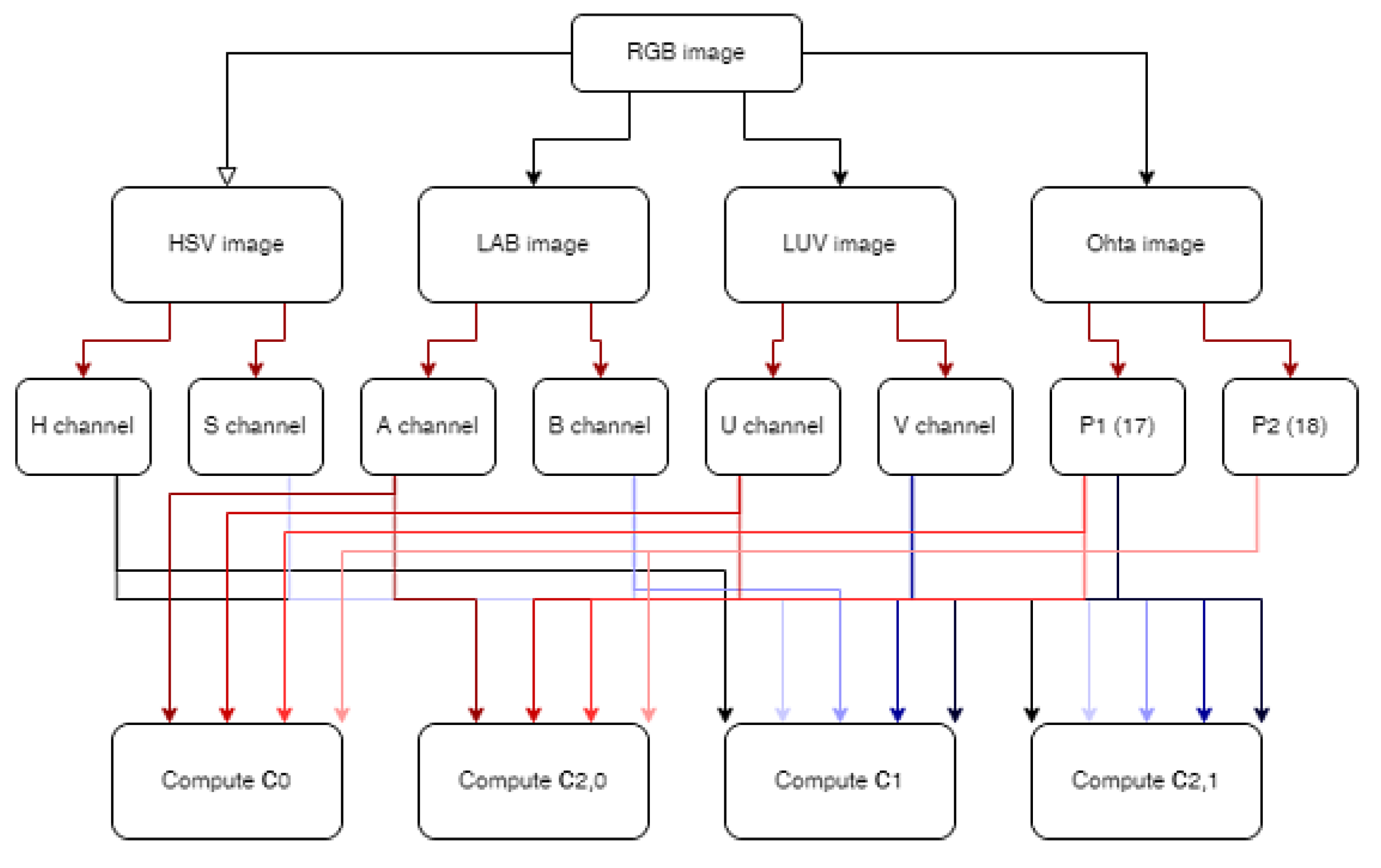
Figure 3.
A test image and its enhanced version (gray scale).


Table 1.
KL divergence of color channels.
| Feature | KL(P(f|c0)||P(f|c2)) | KL(P(f|c1)||P(f|c2)) |
|---|---|---|
| RGB–R channel | 0.67 | 0.58 |
| RGB–G channel | 0.60 | 0.89 |
| RGB–B channel | 0.42 | 1.55 |
| HSV–H channel | 2.45 | 3.22 |
| HSV–S channel | 2.59 | 3.80 |
| HSV–V channel | 0.36 | 0.58 |
| LAB–L channel | 0.63 | 1.05 |
| LAB–A channel | 4.18 | 1.22 |
| LAB–B channel | 1.24 | 4.30 |
| LUV–L channel | 0.60 | 1.06 |
| LUV–U channel | 3.62 | 2.41 |
| LUV–V channel | 0.92 | 3.37 |
| (17) | 3.16 | 7.56 |
| (18) | 5.21 | 2.78 |
Table 2.
Detection accuracy (20) of Selective Search on GTSDB data.
| Method | Danger | Prohibitory | Mandatory |
|---|---|---|---|
| Without enhancement | 0.9206 | 0.9503 | 0.9184 |
| HSI thresholding [9] | 1.0 | 0.9068 | 0.6735 |
| Single-channel norm. [13] | 0.9206 | 0.9503 | 0.9184 |
| Multichannel norm. [10] | 0.9841 | 0.9876 | 0.9592 |
| Our probability model | 1.0 | 1.0 | 0.9592 |
Table 3.
Detection accuracy (20) of Selective Search on the Swedish dataset.
| Method | Warning | Prohibitory | Mandatory |
|---|---|---|---|
| Without enhancement | 1.0 | 0.9739 | 0.9307 |
| HSI thresholding [9] | 0.8814 | 0.9596 | 0.6238 |
| Single-channel norm. [13] | 1.0 | 0.9739 | 0.9307 |
| Multichannel norm. [10] | 0.9492 | 0.9857 | 0.9406 |
| Our probability model | 1.0 | 0.9929 | 0.9802 |
Table 4.
The number of bounding boxes generated on GTSDB data.
| Method | Danger | Prohibitory | Mandatory |
|---|---|---|---|
| Without enhancement | 4689 | 3787 | 4462 |
| HSI thresholding [9] | 977 | 777 | 1180 |
| Single-channel norm. [13] | 4689 | 2794 | 4461 |
| Multichannel norm. [10] | 2458 | 2792 | 3205 |
| Our probability model | 2001 | 2664 | 2858 |
Table 5.
The number of bounding boxes generated on the Swedish dataset.
| Method | Warning | Prohibitory | Mandatory |
|---|---|---|---|
| Without enhancement | 5421 | 36,944 | 20,464 |
| HSI thresholding [9] | 1729 | 12,553 | 6054 |
| Single-channel norm. [13] | 5424 | 36,986 | 20,477 |
| Multichannel norm. [10] | 11,757 | 79,765 | 30,952 |
| Our probability model | 2699 | 14,400 | 8046 |
Table 6.
Average IoU values in percentage.
| Method | Danger | Prohibitory | Mandatory |
|---|---|---|---|
| Faster R-CNN Resnet 50 | 85.04 | 82.52 | 81.21 |
| Faster R-CNN Resnet 101 | 87.05 | 87.29 | 85.58 |
| Faster R-CNN Inception V2 | 85.62 | 82.73 | 79.66 |
| Faster R-CNN Inception Resnet V2 | 90.11 | 91.37 | 89.16 |
| R-FCN Resnet 101 | 86.95 | 87.93 | 85.37 |
| SSD Inception V2 | 85.76 | 81.76 | 80.85 |
| SSD Mobilenet | 81.11 | 80.49 | 78.51 |
| YOLO V2 | 75.82 | 73.96 | 74.66 |
| Selective Search | 78.33 | 78.49 | 77.50 |
| Prob. model + Selective Search | 84.75 | 84.23 | 81.07 |
Table 7.
Average image processing time on the two test devices.
| Device | Avg. Processing Time (s) |
|---|---|
| Computer | 0.07 |
| Raspberry Pi 4 | 1.48 |
Publisher’s Note: MDPI stays neutral with regard to jurisdictional claims in published maps and institutional affiliations. |
© 2022 by the author. Licensee MDPI, Basel, Switzerland. This article is an open access article distributed under the terms and conditions of the Creative Commons Attribution (CC BY) license (https://creativecommons.org/licenses/by/4.0/).
Share and Cite
MDPI and ACS Style
Sütő, J. An Improved Image Enhancement Method for Traffic Sign Detection. Electronics 2022, 11, 871. https://doi.org/10.3390/electronics11060871
AMA Style
Sütő J. An Improved Image Enhancement Method for Traffic Sign Detection. Electronics. 2022; 11(6):871. https://doi.org/10.3390/electronics11060871
Chicago/Turabian StyleSütő, József. 2022. "An Improved Image Enhancement Method for Traffic Sign Detection" Electronics 11, no. 6: 871. https://doi.org/10.3390/electronics11060871
Note that from the first issue of 2016, this journal uses article numbers instead of page numbers. See further details here.