
An Overview of Direction-of-Arrival Estimation Methods Using Adaptive Directional Time-Frequency Distributions


Department of Electrical Engineering, University of Bridgeport, Bridgeport, CT 06604, USA
*
Author to whom correspondence should be addressed.
Electronics 2022, 11(9), 1321; https://doi.org/10.3390/electronics11091321
Submission received: 1 March 2022
/
Revised: 18 April 2022
/
Accepted: 19 April 2022
/
Published: 21 April 2022
(This article belongs to the Section Circuit and Signal Processing)
Abstract
:Direction of arrival (DOA) is one of the essential topics in array signal processing that has many applications in communications, smart antennas, seismology, acoustics, radars, and many more. As the applications of DOA estimation are broadened, the challenges in implementing a DOA algorithm arise. Different environments require different modifications to the existing methods. This paper reviews the DOA algorithms in the literature. It evaluates and compares the performance of the three well known algorithms, including MUSIC, ESPRIT, and Eigenvalue Decomposition (EVD), with and without using adaptive directional time–frequency distributions (ADTFD) at the preprocessing stage. We simulated a case with four sources and three receivers. The sources were well separated. Signals were received at each sensor with an SNR value of −5 dB, 0 dB, 5 dB, and 10 dB. The angles of the sources were 15, 30, 45, and 60 degrees. The simulation results show that the ADTFD algorithm significantly improved the performance of MUSIC, while it did not provide similar results for the ESPRIT and EVD methods. As expected, the computation time of the algorithms was increased by implementing the ADTFD algorithm as a preprocessing step.
1. Introduction
The direction of arrival (DOA) is one of the critical topics in array signal processing. Initially, the DOA was estimated for wireless signals impinging on an array of antennas. Bartlett presented early attempts in 1950 as a periodogram analysis of continuous spectra [1]. Later, Schmidt proposed the Multiple Signal Classification (MUSIC) [2] algorithm in 1986, which is used extensively in DOA estimation. The MUSIC algorithm estimates the frequency content of the received signal using the eigenspace method. In 1989, Roy et al. [3] proposed a new approach known as “the estimation of signal parameters using rotational invariance techniques” (ESPRIT), which exploits the underlying rotational invariance among signal subspaces induced by an array of sensors with a translational invariance structure. It has several advantages over the MUSIC algorithm [3]. Over the years, other researchers proposed many methods and improvements regarding the MUSIC and ESPRIT algorithms and their parameters [4,5]. Advances in machine learning algorithms allowed researchers to develop deep networks for DOA estimation.
The application of DOA is widespread in communication [6], smart antennas, seismology, oceanography [7], acoustics, surveillance, hearing aids, teleconferencing [8], radars, and sonar [9]. As the applications of DOA estimation were broadened, the challenges in implementing the algorithm also arose, such as increased computation time and memory requirements. Different environments require different modifications to the existing methods. In a real-time environment, computational time and cost play an essential role in the application as the military needs the fastest algorithm to estimate the DOA. One of the problems associated with DOA estimation is determining the DOA when there are fewer sensors than the number of sources. This is considered an under-determined case in DOA estimation.
2. Literature Review
Tho et al., proposed a new method to estimate the DOA in an under-determined scenario, which used a combination of noise floor tracking, onset detection, and coherence tests to identify the dominant source in the time-frequency (TF) bin robustly. The most significant eigenvectors of the covariance matrix corresponding to these bins were clustered next. The DOA sources were estimated based on the cluster centroids [10]. Furthermore, some DOA estimation techniques are specifically designed for the environments being used. Dey et al. [11] proposed an application of smart headphones that enabled the selective passing of speech sounds in the environment. Their algorithm was divided into two parts: the first part was a robust far-field speech detection algorithm for noisy environments. The second part was source localization. The application of this technique was a smart headphone system in which a user could be listening to music over headphones and hear speech from a specified direction.
Array structure plays an essential role in DOA estimation. Shi et al. reported that a coprime array, with a different coarray structure, increased the number of degrees of freedom. The proposed sparse reconstruction-based algorithm estimated DOA. In order to improve the power estimation, they modified the sliding window method and removed the spurious peaks in the reconstructed sparse spatial spectrum. Their work showed promising results in DOA and power estimation with achievable degrees of freedom [12]. Zhou et al. proposed a coprime array incorporating compressive sensing. The received signals were compressed by a random compressive sensing kernel to minimize the dimension; then, high-resolution DOA estimation was performed on the compressed measurements. The study verified the computational effectiveness of the method [13]. However, some DOA estimation operations do not consider the spatial relevance among the partitioned coarray statistics [14]. A recent study proposed a coupled coarray tensor canonical polyadic decomposition (CPD)-based 2D DOA estimation to address this. The work used shifting coarray concatenation to factorize the partitioned fourth-order coarray statistics into multiple coupled coarray tensors for the coprime L-shaped array. The number of degrees of freedom (DOF) was increased [14]. Coprime sensor arrays were used in the far-field DOA estimation of the uncorrelated radar signals [15] in order to increase the DOF. The work used the Cuckoo search, which provided an increased number of DOF with low SNR values [14].
Hioka et al. [16] proposed a DOA algorithm depending on the angular resolution and array structure in human–machine interfaces and speech recognition. The efficiency of the proposed algorithm was superior to that of the classical algorithms. Basikolo et al., used a non-uniform circular array to estimate DOA. They used the Khatri-Rao (KR) subspace approach to eliminate spatial noise covariance and estimate DOA with increased degrees of freedom. Using a non-uniform circular array and KR subspace approach, an increased degree of freedom was achieved in estimating the DOA. Because of this, both overdetermined and underdetermined DOA estimation became possible [17]. Xu et al. [18] explored a rectangular array for DOA estimation. The real-valued propagator method was utilized to estimate two-dimensional DOA in their work. As a result, their algorithm provided better angle estimation performance. Zhai et al. [19] employed an unfolded coprime linear array to suppress the ambiguity problem. The received signals from the two sub-arrays were stacked to derive the complete signal subspace. The authors introduced a reduced dimensional MUSIC algorithm (RD-MUSIC) for noncircular signals impinging on the two sub-arrays, which increased the noncircular signals’ accuracy [19].
Feng et al., 2001, proposed a DOA estimation algorithm for wideband signals [20]. Their algorithm used fast chirplet-based adaptive signal decomposition to build a time–frequency covariance matrix. Subspace fitting was conducted similar to that of traditional MUSIC and ESPRIT algorithms. The authors overlapped the narrow and wideband incoherent subspace and built a general TF matrix in this work. A wideband DOA estimation algorithm using fast Chirplet-based adaptive signal decomposition was projected based on the differences. The advantages of using this algorithm were that there was no restriction for array structure with very low complexity and robust performance.
Time-frequency analysis provides information in both the time domain as well as in the frequency domain. One such method used spatial TF distributions in a wideband scenario. This approach used spatial pseudo-Wigner–Ville distribution to analyze the time and frequency domain signals. The proposed method outperformed methods for FM signals and performed significantly better for wideband signals [21].
Bouri proposed a method using factorizations of a sample cross-spectral matrix for detecting and localizing the sources. This technique did not use eigenvalue decomposition to reduce computational cost and improve performance [22].
Mohan et al., suggested a new method to localize multiple speech sources with small arrays using a coherence test [8]. The authors proposed two methods: (1) narrowband spatial spectrum estimation at each bin followed by summation of directional spectra across time and frequency and (2) clustering low-rank covariance matrices and averaging the covariance matrices within the clusters [8]. However, there are many other approaches used to estimate DOA via different methods. Nishiura et al. [23] designed two other methods apart from the classical methods to estimate the DOA. The first method was DOA estimation based on a cross power spectrum phase and the second method was a statistical sound source identification algorithm based on the Gaussian mixture model. The above methods were used to localize the source signal by enhancing multiple sound signals. A microphone array had to be steered, for which the delay-and-sum beamformer method was employed to localize the source [23]. Sawada et al., proposed an approach for DOA estimation using independent component analysis. They reported that independent component analysis identified source signals from their mixture. The work stated the main advantage of independent component analysis over the MUSIC algorithm was that it could be applied even when the number of sources was equal to the number of sensors [24]. Matsuo et al., implemented a histogram mapping method to estimate the DOA of multiple speech signals.
The significant advantages of the histogram mapping method included low computational complexity and no requirement for the preliminary DOA estimates [25]. The authors introduced a mechanism to delete narrowband components present in the vector analysis. Swartling et al. [9] improved a statistical method known as steered response power with phase transform (SRP-PHAT) for DOA estimation. SRP-PHAT uses second-order statistics through cross power spectra to navigate a beamformer, searching for a maximum power output [9]. A peak in the beamformer was aimed towards the acoustic source with the highest power. Swartling et al. stated that fourth-order statistics provided a route to distinguish speech from noise. The fourth-order statistics provided superior performance compared to the second-order statistics, but the computation complexity doubled.
Wang and Zhang developed an iterative positioning algorithm to solve the link blockage problem in mmWave communication systems. As the first step, they used random beamforming and maximum likelihood estimation to estimate the angle of arrival and the angle of departure. Their proposed iterative algorithm achieved centimeter-level positioning accuracy [26].
Compressed sensing (CS) methods, on-grid, off-grid, and grid-less, use the signal sources’ characteristics in the spatial domain. On-grid and off-grid methods have grid mismatch problems resulting in performance loss [27]. However, these two methods have less computational complexity. On the other hand, gridless methods perform better but have higher computational complexity [28].
In recent years, machine learning-based DOA estimation algorithms were proposed, including deep neural networks (DNN) and convolutional neural networks (CNN) [29,30,31,32,33]. Kase et al., developed a DNN-based DOA estimation of two targets [29]. They used a correlation matrix Rxx as an input and tested the proposed DNN for a case with two targets, and both narrowband signals from the targets were uncorrelated and had equal power. DNN-based methods require training. Kase et al. generated the training data by changing the SNR in pre-determined patterns in the range of 0–30 dB. They reported that the designed DNN achieved very high performance for the same case. This verified the well-known fact that the DNN-based solutions’ performance highly depends on the training data and is susceptible to overfitting problems.
Liu et al. [30] proposed DOA estimation for underwater acoustic signals with different waves using a CNN architecture that uses the covariance matrix Rxx as the input array. To prevent the neural network from dealing with complex numbers, they divided the covariance matrix into two channels: real number and imaginary number layers. After training, the method was tested under a scenario in which different array elements were simulated under different water environment conditions with SNR of 20 dB, 10 dB, 0 dB, and −10 dB. The paper reported accuracy rates comparable to the MUSIC algorithm and reduced the estimation time of the DOA by 10 times less than the MUSIC algorithm. Liu et al. argued that their proposed CNN-based DOA estimation method was “far better than the traditional MUSIC algorithm” and was especially suitable for the underwater acoustic environment [30]. The environment’s complex and changeable characteristics require a shorter calculation time and good accuracy in DOA estimation. However, the authors missed that the neural network-based DOA estimation algorithms’ performance exclusively depends on training data, and complex and changeable environment characteristics negatively affect such algorithms.
There are several preprocessing techniques performed before DOA estimation, such as speech enhancement based on the subspace method [34], blind source separation [35,36], sub-band-based clustering [37], and the adaptive directional time–frequency distributions (ADTFD) method [38].
The technique introduced by Asano et al. [34] constituted two stages corresponding to the different types of noise. In the first stage, ambient noise, which was less directional, was reduced by eliminating the noise-dominant subspaces. In the second stage, the spectrum of the target source was extracted from the multi-directional components. Visser et al. proposed a method for speech enhancement in a noisy environment. A practical application in a car was experimented with [35]. Their approach included combining two techniques, namely blind source separation and speech denoising, using hybrid wavelet independent component analysis. Blind source separation exploited the time correlation of speech signals captured by microphones. Blind source separation was used to locate the point source. Independent component analysis was used for the adaptive denoising of the separated signals. Mitianoudis et al., also used blind source separation for audio source separation. The authors introduced a technique for unmixing audio sources in an auditory scene [36]. Khan et al., reported that ADTFD performed well in analyzing close signal components compared to the other preprocessing methods. The ADTFD optimized the direction of the kernel at each point in the TF domain to obtain a clear representation, which was then exploited for DOA estimation [38].
Postprocessing methods may be employed after DOA estimation. Some of the commonly used postprocessing methods are postfiltering algorithms. Habets et al. [39] proposed a postfiltering algorithm for the spectral enhancement of speech signals. A feature of this technique was reduced interference. Gu et al., suggested a technique that used the QR decomposition-based recursive least square (QRD-RLS) technique as postprocessing. QRD-RLS was used to estimate the DOA from the autoregressive sources estimated employing the Kalman filter. Auto-regressive modeled sources provide excellent temporal information, enabling the QRD-RLS technique to estimate the DOAs. [40].
In the literature, Khan et al. [38] reported that the algorithm was applicable to sub-space-based DOA methods. However, they assessed the ADTFD only for MUSIC. One of the goals of this paper is to compare the performances of three well known DOA estimation methods, including MUSIC, ESPRIT, and Eigenvalue Decomposition (EVD), by implementing ADTFD in the preprocessing stage. Another goal is to overview the existing DOA algorithms.
3. DOA Estimation Algorithms
3.1. The MUSIC Algorithm
Schmidt (1986) proposed the MUSIC algorithm [2], which is a subspace-based method. MUSIC stands for multiple signal classification. The MUSIC algorithm provides asymptotically unbiased estimates of the number of signals, directions of arrival (DOA), strengths and cross-correlations between the directional waveforms, polarizations, and strength of noise or interference. The model in Figure 1 states that the waveforms received at the M-array elements are linear combinations of the D incident wavefronts and noise.
Vector represents the incident signals in amplitude and phase at some arbitrary reference point. Vector is the sensed or generated noise. Matrix , in Equations (1)–(3), contains elements such as and The columns in matrix A are called mode vectors and represent responses to the direction of arrival, for example, is the direction of arrival of the signal. The solution of the DOA of multiple signals includes locating the intersections of the continuum with the range space of The covariance matrix of the X vector is and is defined as
Note that (.)* is used to denote the Hermitian conjugate or complex conjugate transpose operation. The MUSIC algorithm assumes that incident signals and noise are uncorrelated. The matrix may be diagonal and singular. In the case of the number of wavefronts, D is less than the number of array elements , is a nonnegative definite, and its rank is less than . The Equation (7) is satisfied when λ is one of the eigenvalues of in the metric of . λ is the minimum eigenvalue .
If the elements of the noise vector are mean zero,
the signal correlation matrix is not necessarily diagonal since the incident signals are either somewhat correlated or uncorrelated. This method implies either knowing the number of incoming signals in advance or searching the eigenvalues to determine the number of incoming signals. If the number of signals is , the number of signal eigenvalues and eigenvectors is , and the number of noise eigenvalues and eigenvectors is ( is the number of array elements). is an M × M matrix. After the computation of the array correlation matrix, , we must find the eigenvalues and eigenvectors for . From the eigenvectors computed, eigenvectors are associated with the signals, and eigenvectors are associated with the noise. We further deal with the eigenvectors associated with the noise that have the smallest corresponding eigenvalues from the set of eigenvalues of . For uncorrelated signals, the smallest eigenvalues are equal to the variance of the noise. The following equation defines the noise subspace.
The eigenvectors of the signal subspace and the noise subspace are orthogonal to each other. This is the essential observation of the MUSIC approach. Since the steering vectors corresponding to signal components are orthogonal to the noise subspace, the DOA of the multiple incident signals can be estimated by locating the peaks of the spatial spectrum given by
The flowchart of the MUSIC algorithm is summarized in Figure 2. The MUSIC algorithm’s performance is different when the received signals are different. The MUSIC algorithm fails to detect correlated input signals as the response of the MUSIC is not sharp at the peaks while it is sharp in the case of the uncorrelated input signal [16].
3.2. The ESPRIT Algorithm
Another subspace-based algorithm, which was an improvement over the MUSIC algorithm, was proposed by Roy et al. (1989) [3]. ESPRIT stands for the estimation of signal parameters via rotational invariance techniques. It does not require knowledge of the array geometry and does not involve an exhaustive search through all possible steering vectors to estimate DOA. Hence, it reduces the computational and storage requirements significantly compared to the MUSIC algorithm. ESPRIT exploits an underlying rotational invariance among signal subspaces induced by an array of sensors with a translational invariance structure. This algorithm is more robust for array imperfections than the MUSIC algorithm. Consequently, the computational complexity and storage requirements are lower [6]. It also explores the rotational invariance property in the signal subspace created by two subarrays derived from the original array with a translational invariance structure. Unlike the MUSIC method, ESPRIT simultaneously estimates the number of antenna elements and DOAs. Figure 3 illustrates the ESPRIT algorithm’s DOA estimation with multiple sources.
Although the ESPRIT algorithm has many advantages, it is not entirely general, as it has restrictions on planar wavefronts and pairwise matched co-directional doubles. ESPRIT describes the array as being comprised of two subarrays, X and Y, to exploit the sensor array’s translational invariance property. The subarrays X and Y are identical but physically displaced by a known displacement vector. The received signals are represented as:
is the signal as received at the reference sensor of the X subarray. is the DOA of the source relative to the direction of the translational displacement vector. is defined as the magnitude of the displacement vector between the two arrays, and c is the speed of propagation in the transmission medium. and are the noise signals in the doublet for the subarrays, respectively.
The auto-covariance matrix and the cross-covariance matrix are defined as below.
Once is calculated, the DOAs are calculated as:
3.3. Eigenvector Clustering Algorithm
Eigenvector clustering is another method used for DOA estimation [10]. Preprocessing is a critical step to eliminate noise vectors in the covariance matrix. The method uses the short-time Fourier transform (STFT), noise floor tracking, onset detection, and coherence test. DOA estimation is performed using the data from the cluster centroids. The array structure is also specified in this method. A triangular array with three microphones at a right angle is employed. The STFT of the multi-component signal is the first step to estimating the time-frequency (TF) bins in each frequency component. A speech enhancement method is used to select TF bins based on the speech enhancement method using a certain threshold value [7,9]. The onset is marked by a sudden rise in the energy of particular frequency bands and is used to detect sudden sound activity. Many onset detection functions detect the changes in one or more signal properties, considering that signals, specifically audio, have constantly changing properties such as amplitude, noise, onsets, offsets, and vibration. The onset of a signal increases the energy in the time domain [41] and in the frequency bands that other properties do not have. Therefore, an increase in energy in some frequency bands can be employed as an indicator of onset [16]. The coherence test proposed by Mohan et al. [8] is applied to select rank-1 TF bins. Rank-TF bins are selected since only one source dominates that particular TF bin. It means that only TF bins with a possibility of the incoming signal are present. The DOAs can be estimated from the cluster centroids after clustering the largest eigenvectors, based on the structure of the steering vectors and the microphone arrangement. Once noise-tracking and onset detection are performed, the method selects rank-1 TF bins, and most of the covariance matrices can be approximated. Eigenvalues and eigenvectors of the covariance matrix are determined. The algorithm clusters the normalized matrix into several clusters equal to the number of sources. Finally, the DOAs are estimated.
4. Adaptive Directional Time–Frequency Distributions (ADTFD)
Many applications use non-stationary signals that exhibit time-varying frequency spectra. The spatial time–frequency distribution (STFD) is a well-known approach for analyzing non-stationary multi-sensor signals. Since the STFD matrices contain high energy points in the TF domain, they result in a robust DOA estimation against noisy disturbances [42,43,44,45]. Many studies reported improved DOA estimation for the conventional MUSIC algorithm by replacing covariance matrices with the STFD matrices [42,43,46]. The selection of the TF presenters for the sources improves the DOA estimation, where the number of sensors is less than the number of sources, which is called an under-determined case. In such cases, separate STFDs are constructed, each corresponds to one source, and they are used to estimate DOAs [47,48]. The estimated instantaneous frequency (IF) is used to obtain the sources’ TF presenters. Spatially averaged time–frequency distribution (TFD) of sensor information is employed to estimate the IF [47,49,50]. The benefits of TFDs can be summarized as follows:
(a) In traditional signal representations, time and frequency are mutually exclusive, and each representation is non-localized with respect to the other representation. Only one domain representation may become insufficient for complex problems. In such cases, the distribution of time and frequency may present additional information.
(b) TFDs allow the analysis of the signals representing the signal characteristics such as relative amplitudes, IF, complexity, flatness, and energy distribution in the TF domain [51].
The resolution of the TFD plays an essential role in DOA estimation, mainly when the sources are closely located. Both the STFD and TF filter approaches heavily depend on the TFD’s resolution, which has higher computational cost and memory requirements. A DOA approach using the ADTFD, proposed by Khan et al., provided good improvements for non-stationary signals and the MUSIC algorithm [38]. The algorithm, illustrated in Figure 4, consists of several stages, including calculating and averaging TFDs, IF estimation, and TF filtering. Quadratic TFD is used to analyze the signals. The estimated IF components are used to design TF filtering [33,38].
4.1. Spatial Averaging of TFDs
Wigner–Ville Distribution (WVD), is used to calculate the TFDs of a signal. It is defined as
is the analytic associate of the signal, and it is complex. WVD is used to study non-stationary signals. Considering that DOA deals with non-stationary signals, WVD becomes useful in DOA estimation. Averaging TFDs is performed by dividing by the number of array elements.
Postprocessing is performed to preserve the energy of weak TFD components while resolving the closely-spaced components. It allows accurate IF extraction. An adaptive smoothing kernel is applied to the in order to resolve close components of the signal. Then, the ADTFD is defined using the average TFD and the second derivative directional Gaussian filter.
4.2. Multi-Component Analysis
Multi-component analysis consists of IF estimation and TF filtering. The IF of a signal indicates the dominant frequency of the signal at a given time. The peaks of the multi-component signal in the TF domain are used to estimate the IF. The peaks are calculated by setting the first and second derivatives of the ADTFD to zero. The phase is estimated by TF filtering on the estimated IFs [38].
5. Special Case: Experimental Results and Discussions
We simulated a case that had four sources with three receivers. The sources are well separated and represented as follows:
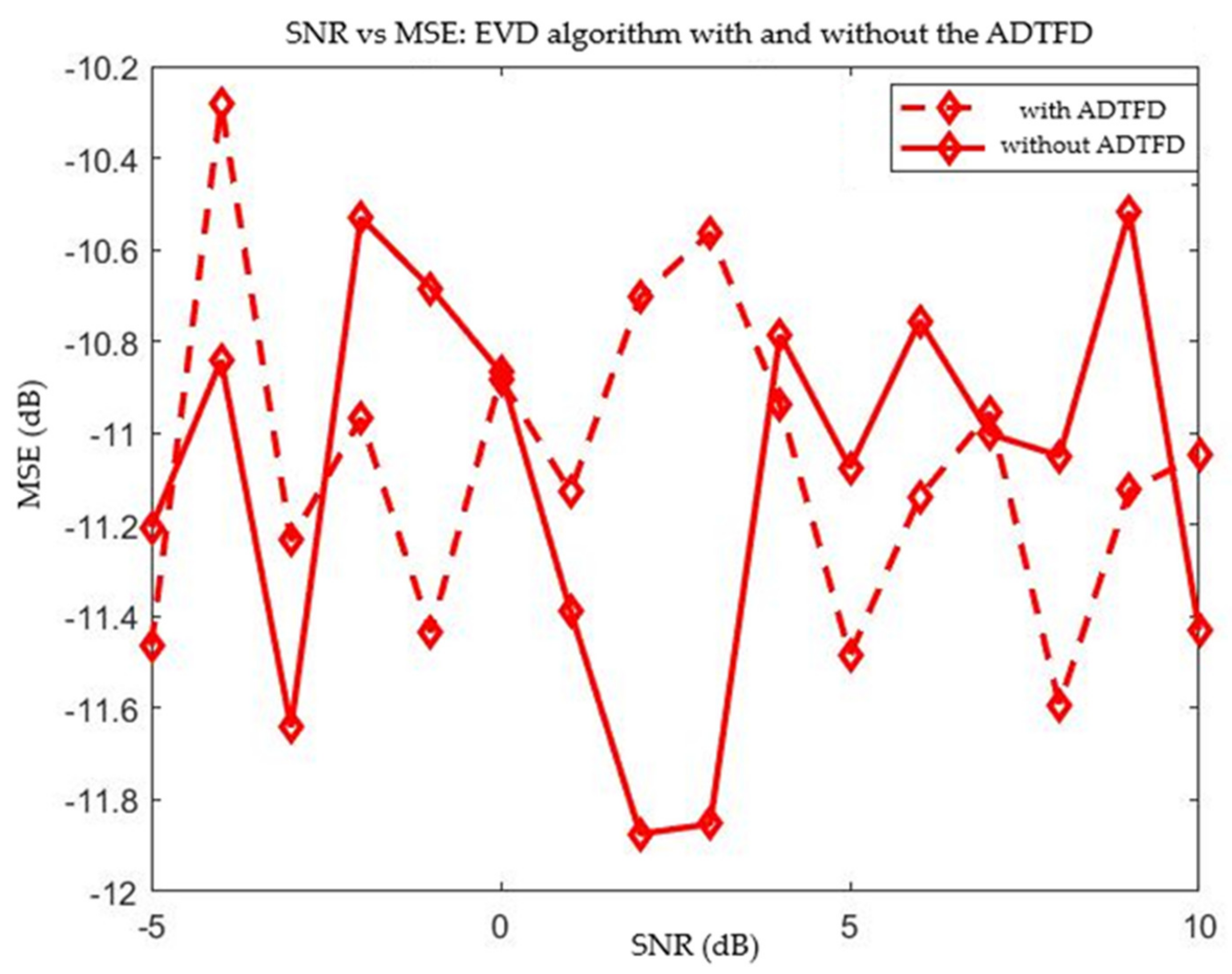
w(t) represents the Gaussian noise. Signals are received at each sensor with an SNR value of −5 dB, 0 dB, 5 dB, or 10 dB. The angles of the sources are 15, 30, 45, and 60 degrees. The performances of the reviewed DOA methods, MUSIC, ESPRIT, and Eigenvalue Decomposition (EVD), are given in Table 1 and Table 2 with and without the ADTFD algorithm, respectively. The EVD algorithm performed better than the MUSIC and ESPRIT algorithms in estimating the DOAs without the ADTFD under different SNR values. Corresponding mean square error (MSE) values in dB are depicted in Figure 5. The EVD algorithm’s MSE values were around −11 dB, while the ESPRIT algorithm’s MSE values were around −3 dB. The MUSIC algorithm produced a steady MSE of about −8.2 dB for different SNR values. The ADTFD algorithm in the preprocessing stage improved the MUSIC algorithm’s performance significantly. On the other hand, the ESPRIT and EVD algorithms did not benefit from the ADTFT. The DOAs are given in Table 2. The MSE versus SNR plot for the DOA algorithms with the ADTFD for different SNR values is shown in Figure 6. The MSE values of the MUSIC were calculated below −22 dB with the ADTFD.
We can see the effect of the ADTFD preprocessing algorithm on each DOA method more clearly in Figure 7, Figure 8 and Figure 9. The ESPRIT and EVD methods’ MSE values did not improve with the ADTFD. The average unoptimized computation time for ADTFD using the MUSIC algorithm is 1.83 s and for the EVD is 1.66 s on a system using 16 GB RAM. The results are summarized in Table 3.
6. Conclusions
This work reviewed the DOA estimation algorithms in the literature. Furthermore, it simulated a case that had four well-separated sources with three receivers. Signals were received at each sensor with SNR values of −5 dB, 0 dB, 5 dB, and 10 dB. The angles of the sources were 15, 30, 45, and 60 degrees. The performances of the MUSIC, ESPRIT, and Eigenvalue Decomposition (EVD) algorithms were evaluated and compared with and without using the ADTFD algorithm. The ADTFD algorithm is a preprocessing step before the DOA estimation. It was originally developed for the MUSIC algorithm, but its effects on the other DOA estimation methods are not often studied. Our simulation results showed that the EVD algorithm performed better than the MUSIC and ESPRIT algorithms in estimating the DOAs without the ADTFD under different SNR values. However, the ADTFD algorithm improved the performance of the MUSIC algorithm significantly while not affecting the other DOA estimation methods. As expected, the computation time of the methods increased by using the ADTFD algorithm.
Author Contributions
P.K.E. and B.D.B. contributed equally to this work. All authors have read and agreed to the published version of the manuscript.
Funding
This research received no external funding.
Conflicts of Interest
The authors declare no conflict of interest.
References
- Bartlett, M.S. Periodogram Analysis and Continuous Spectra. Biometrika 1950, 37, 1–16. [Google Scholar] [CrossRef] [PubMed]
- Schmidt, R. Multiple emitter location and signal parameter estimation. IEEE Trans. Antennas Propag. 1986, 34, 276–289. [Google Scholar] [CrossRef] [Green Version]
- Roy, R.; Paulraj, A.; Kailath, T. Estimation of Signal Parameters via Rotational Invariance Techniques—Esprit. In Proceedings of the Nineteeth Asilomar Conference on Circuits, Systems and Computers, Pacific Grove, CA, USA, 6–8 November 1985; pp. 41.6.1–41.6.5. [Google Scholar]
- Wang, R.; Wang, Y.; Li, Y.; Cao, W.; Yan, Y. Geometric Algebra-Based ESPRIT Algorithm for DOA Estimation. Sensors 2021, 21, 5933. [Google Scholar] [CrossRef]
- Luan, S.; Li, J.; Gao, Y.; Zhang, J.; Qiu, T. Generalized covariance-based ESPRIT-like solution to direction of arrival estimation for strictly non-circular signals under Alpha-stable distributed noise. Digit. Signal Process. 2021, 118, 103214. [Google Scholar] [CrossRef]
- Mankal, P.; Gowre, S.C.; Dakulagi, V. A New DOA Algorithm for Spectral Estimation. Wirel. Pers. Commun. 2021, 119, 1729–1741. [Google Scholar] [CrossRef]
- Al Mahmud, T.H.; Ye, Z.; Shabir, K.; Sheikh, Y.A. DOA Estimation of Quasi-Stationary Signals Exploiting Virtual Extension of Coprime Array Imbibing Difference and Sum Co-Array. IEICE Trans. Commun. 2018, E101.B, 18761883. [Google Scholar] [CrossRef]
- Mohan, S.; Lockwood, M.E.; Kramer, M.L.; Jones, D.L. Localization of multiple acoustic sources with small arrays using a coherence test. J. Acoust. Soc. Am. 2008, 123, 2136–2147. [Google Scholar] [CrossRef] [Green Version]
- Swartling, M.; Sallberg, B.; Grbic, N. Direction of arrival estimation for speech sources using fourth order cross cumulants. In Proceedings of the 2008 IEEE International Symposium on Circuits and Systems (ISCAS), Seattle, WA, USA, 18–21 May 2008; pp. 1696–1699. [Google Scholar] [CrossRef] [Green Version]
- Tho, N.T.N.; Zhao, S.; Jones, D.L. Robust DOA estimation of multiple speech sources. In Proceedings of the 2014 IEEE International Conference on Acoustics, Speech and Signal Processing (ICASSP), Florence, Italy, 4–9 May 2014; pp. 2287–2291. [Google Scholar]
- Dey, A.; Nandi, A.; Basu, B. Gold-MUSIC based DOA estimation using ULA antenna of DS-CDMA sources with propagation delay diversity. AEU Int. J. Electron. Commun. 2018, 84, 162–170. [Google Scholar] [CrossRef]
- Shi, Z.; Zhou, C.; Gu, Y.; Goodman, N.A.; Qu, F. Source Estimation Using Coprime Array: A Sparse Reconstruction Perspective. IEEE Sens. J. 2017, 17, 755–765. [Google Scholar] [CrossRef]
- Zhou, C.; Gu, Y.; Zhang, Y.D.; Shi, Z.; Jin, T.; Wu, X. Compressive sensing-based coprime array direction-of-arrival estimation. IET Commun. 2017, 11, 1719–1724. [Google Scholar] [CrossRef]
- Zheng, H.; Shi, Z.; Zhou, C.; Haardt, M.; Chen, J. Coupled Coarray Tensor CPD for DOA Estimation with Coprime L-Shaped Array. IEEE Signal Process. Lett. 2021, 28, 1545–1549. [Google Scholar] [CrossRef]
- Hameed, K.; Khan, W.; Abdalla, Y.S.; Al-Harbi, F.F.; Armghan, A.; Asif, M.; Salman Qamar, M.; Ali, F.; Miah, M.S.; Alibakhshikenari, M.; et al. Far-Field DOA Estimation of Uncorrelated RADAR Signals through Coprime Arrays in Low SNR Regime by Implementing Cuckoo Search Algorithm. Electronics 2022, 11, 558. [Google Scholar] [CrossRef]
- Hioka, Y.; Hamada, N. DOA estimation of speech signal using equilateral-triangular microphone array. In Proceedings of the 8th European Conference on Speech Communication and Technology, Geneva, Switzerland, 1–4 September 2003; pp. 1717–1720. [Google Scholar]
- Basikolo, T.; Ichige, K.; Arai, H. Direction of arrival estimation for quasi-stationary signals using nested circular array. In Proceedings of the 2016 4th International Workshop on Compressed Sensing Theory and its Applications to Radar, Sonar and Remote Sensing (CoSeRa), Aachen, Germany, 19–22 September 2016; pp. 193–196. [Google Scholar]
- Xu, L.; Wen, F. Fast Noncircular 2D-DOA Estimation for Rectangular Planar Array. Sensors 2017, 17, 840. [Google Scholar] [CrossRef] [Green Version]
- Zhai, H.; Zhang, X.; Zheng, W.; Gong, P. DOA Estimation of Noncircular Signals for Unfolded Coprime Linear Array: Identifiability, DOF and Algorithm. IEEE Access 2018, 6, 29382–29390. [Google Scholar] [CrossRef]
- Aigang, F.; Zheng, Z.; Qinye, Y. Wideband direction-of-arrival estimation using fast chirplet-based adaptive signal decomposition algorithm. In Proceedings of the IEEE 54th Vehicular Technology Conference. VTC Fall 2001. Proceedings (Cat. No.01CH37211), Atlantic City, NJ, USA, 7–11 October 2001; pp. 1432–1436. [Google Scholar]
- Gershman, A.B.; Amin, M.G. Wideband direction-of-arrival estimation of multiple chirp signals using spatial time-frequency distributions. IEEE Signal Process. Lett. 2000, 7, 152–155. [Google Scholar] [CrossRef]
- Bouri, M. Source Detection and Localization in Array Signal Processing. In Proceedings of the First International Symposium on Environment Identities and Mediterranean Area, Corte-Ajaccio, France, 9–12 July 2006; pp. 12–17. [Google Scholar] [CrossRef]
- Nishiura, T.; SNakamura, S.; Shikano, K. Talker localization in a real acoustic environment based on DOA estimation and statistical sound source identification. In Proceedings of the IEEE International Conference on Acoustics, Speech, and Signal Processing, Orlando, FL, USA, 13–17 May 2002; pp. I-893–I-896. [Google Scholar] [CrossRef] [Green Version]
- Sawada, H.; Mukai, M.; Makino, S. Direction of arrival estimation for multiple source signals using independent component analysis. In Proceedings of the Seventh International Symposium on Signal Processing and Its Applications, Paris, France, 4 July 2003; pp. 411–414. [Google Scholar] [CrossRef] [Green Version]
- Matsuo, M.; Hioka, Y.; Hamada, N. Estimating DOA of Multiple Speech Signals by Improved Histogram Mapping Method. In Proceedings of the International Workshop on Acoustic Echo and Noise Control (IWAENC), High Tech Campus, Eindhoven, The Netherlands, 12–15 September 2005; pp. 129–132. [Google Scholar]
- Wang, W.; Zhang, W. Joint beam training and positioning for intelligent reflecting surfaces assisted millimeter-wave communications. IEEE Trans. Wirel. Commun. 2021, 20, 6282–6297. [Google Scholar] [CrossRef]
- Chi, Y.; Scharf, L.L.; Pezeshki, A.; Calderbank, A.R. Sensitivity to basis mismatch in compressed sensing. IEEE Trans. Signal Process. 2011, 59, 2182–2195. [Google Scholar] [CrossRef]
- Yang, Z.; Xie, L.; Zhang, C. A discretization-free sparse and parametric approach for linear array signal processing. IEEE Trans. Signal Process. 2014, 62, 4959–4973. [Google Scholar] [CrossRef] [Green Version]
- Kase, Y.; Nishimura, T.; Ohgane, T.; Ogawa, Y.; Kitayama, D.; Kishiyama, Y. DOA Estimation of Two Targets with Deep Learning. In Proceedings of the 15th Workshop on Positioning, Navigation and Communications (WPNC), Bremen, Germany, 25–26 October 2018; pp. 1–5. [Google Scholar] [CrossRef]
- Liu, Y.; Chen, H.; Wang, B. DOA estimation based on CNN for underwater acoustic array. Appl. Acoust. 2021, 172, 107594. [Google Scholar] [CrossRef]
- Lin, L.; She, C.; Chen, Y.; Guo, Z.; Zeng, X. TB-NET: A Two-Branch Neural Network for Direction of Arrival Estimation under Model Imperfections. Electronics 2022, 11, 220. [Google Scholar] [CrossRef]
- Hoang, D.T.; Lee, K. Deep Learning-Aided Coherent Direction-of-Arrival Estimation with the FTMR Algorithm. IEEE Trans. Signal Process. 2022, 70, 1118–1130. [Google Scholar] [CrossRef]
- Papageorgiou, G.K.; Sellathurai, M.; Eldar, Y.C. Deep Networks for Direction-of-Arrival Estimation in Low SNR. IEEE Trans. Signal Process. 2021, 69, 3714–3729. [Google Scholar] [CrossRef]
- Asano, F.; Hayamizu, S.; Yamada, T.; Nakamura, S. Speech enhancement based on the subspace method. IEEE Trans. Speech Audio Process. 2000, 8, 497–507. [Google Scholar] [CrossRef] [Green Version]
- Visser, E.; Lee, T.; Otsuka, M. Speech enhancement in a noisy car environment. In Proceedings of the 3rd International Conference on Independent Component Analysis and Source Separation, San Diego, CA, USA, 9–13 December 2001; pp. 272–277. [Google Scholar]
- Mitianoudis, N.; Davies, M.E. Audio source separation: Solutions and problems. Int. J. Adapt. Control Signal Process. 2004, 18, 299–314. [Google Scholar] [CrossRef]
- Yermeche, Z.; Grbic, N.; Claesson, I. Speech enhancement of multiple moving sources based on subband clustering time-delay estimation. In Proceedings of the International Workshop on Acoustic Echo and Noise Control (IWAENC), Paris, France, 12–14 September 2006; pp. 1–4. [Google Scholar]
- Ali Khan, N.; Ali, S.; Jansson, M. Direction of arrival estimation using adaptive directional time-frequency distributions. Multidimens. Syst. Signal Process. 2018, 29, 503–521. [Google Scholar] [CrossRef]
- Habets, E.A.R.; Gannot, S. Dual-Microphone Speech Dereverberation using a Reference Signal. In Proceedings of the 2007 IEEE International Conference on Acoustics, Speech and Signal Processing (ICASSP ’07), Honolulu, HI, USA, 15–20 April 2007; pp. IV-901–IV-904. [Google Scholar] [CrossRef] [Green Version]
- Gu, J.; Chan, S.C.; Zhu, W.; Swamy, M.N.S. Joint DOA Estimation and Source Signal Tracking with Kalman Filtering and Regularized QRD RLS Algorithm. IEEE Trans. Circuits Syst. II 2013, 60, 46–50. [Google Scholar] [CrossRef]
- Bachu, R.; Kopparthi, S.; Adapa, B.; Barkana, B. Voiced/Unvoiced Decision for Speech Signals Based on Zero-Crossing Rate and Energy. In Advanced Techniques in Computing Sciences and Software Engineering; Springer: Dordrecht, The Netherlands, 2010. [Google Scholar] [CrossRef]
- Amin, M.G.; Zhang, Y. Direction finding based on spatial time-frequency distribution matrices. Digit. Signal Process. 2000, 10, 325–339. [Google Scholar] [CrossRef] [Green Version]
- Zhang, Y.; Ma, W.; Amin, M. Subspace analysis of spatial time-frequency distribution matrices. IEEE Trans. Signal Process. 2001, 49, 747–759. [Google Scholar] [CrossRef] [Green Version]
- Chabriel, G.; Kleinsteuber, M.; Moreau, E.; Shen, H.; Tichavsky, P.; Yeredor, A. Joint matrices decompositions and blind source separation: A survey of methods, identification, and applications. IEEE Signal Process. Mag. 2014, 31, 34–43. [Google Scholar] [CrossRef]
- Belouchrani, A.; Amin, M. Time-frequency MUSIC. IEEE Signal Process. Lett. 1999, 6, 109–110. [Google Scholar] [CrossRef]
- Belouchrani, A.; Amin, M.; Thirion-Moreau, N.; Zhang, Y. Source separation and localization using time-frequency distributions: An overview. IEEE Signal Process. Mag. 2013, 30, 97–107. [Google Scholar] [CrossRef]
- Heidenreich, P.; Cirillo, L.; Zoubir, A. Morphological image processing for FM source detection and localization. Signal Process. 2009, 89, 1070–1080. [Google Scholar] [CrossRef]
- Sharif, W.; Chakhchoukh, Y.; Zoubir, A. Robust spatial time-frequency distribution matrix estimation with application to direction-of-arrival estimation. Signal Process. 2011, 91, 2630–2638. [Google Scholar] [CrossRef]
- Rankine, L.; Mesbah, M.; Boashash, B. IF estimation for multicomponent signals using image processing techniques in the time-frequency domain. Signal Process. 2007, 87, 1234–1250. [Google Scholar] [CrossRef] [Green Version]
- Zhang, H.; Bi, G.; Yang, W.; Razul, S.; See, C. IF estimation of FM signals based on time-frequency image. IEEE Trans. Aerosp. Electron. Syst. 2015, 51, 326–343. [Google Scholar] [CrossRef]
- Boashash, B. Time-Frequency Signal Analysis and Processing, a Comprehensive Reference. In EURASIP and Academic Press Series in Signal and Image Processing; Academic Press: Cambridge, MA, USA, 2016. [Google Scholar]
Figure 1.
DOA estimation using the MUSIC algorithm.

Figure 2.
Flowchart for the MUSIC algorithm.
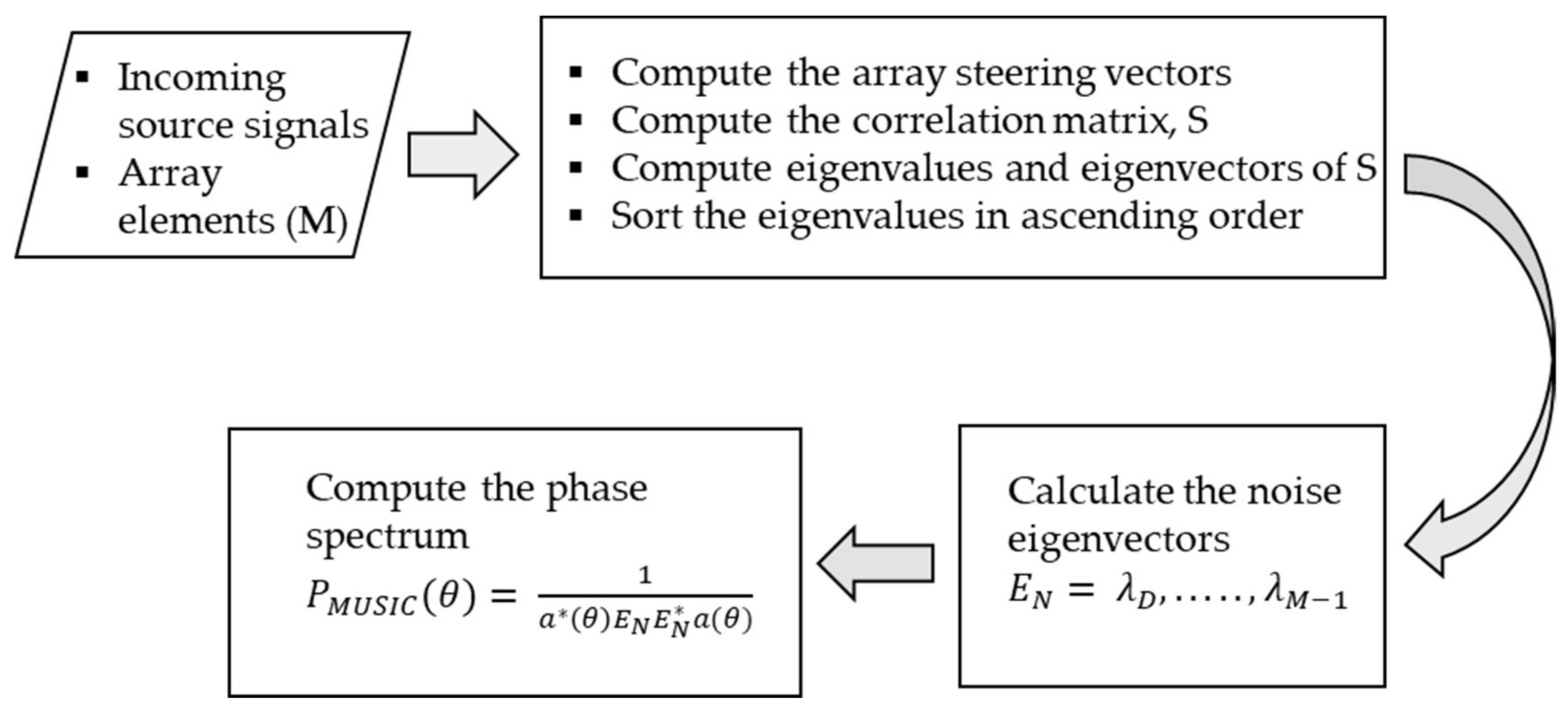
Figure 3.
Multiple source DOA estimation using the ESPRIT algorithm.

Figure 4.
Illustration of the ADTFD algorithm with the DOA estimation stage.

Figure 5.
SNR vs. MSE plot of the MUSIC, ESPRIT, and Eigenvalue Decomposition algorithms without the ADTFD preprocessing algorithm.
Figure 5.
SNR vs. MSE plot of the MUSIC, ESPRIT, and Eigenvalue Decomposition algorithms without the ADTFD preprocessing algorithm.

Figure 6.
SNR vs. MSE plot of the MUSIC, ESPRIT, and EVD algorithms using the ADTFD.

Figure 7.
SNR vs. MSE plot of the MUSIC algorithm with and without ADTFD (solid line and the dashed line represents the cases without ADTFT and with ADTFD, respectively).
Figure 7.
SNR vs. MSE plot of the MUSIC algorithm with and without ADTFD (solid line and the dashed line represents the cases without ADTFT and with ADTFD, respectively).
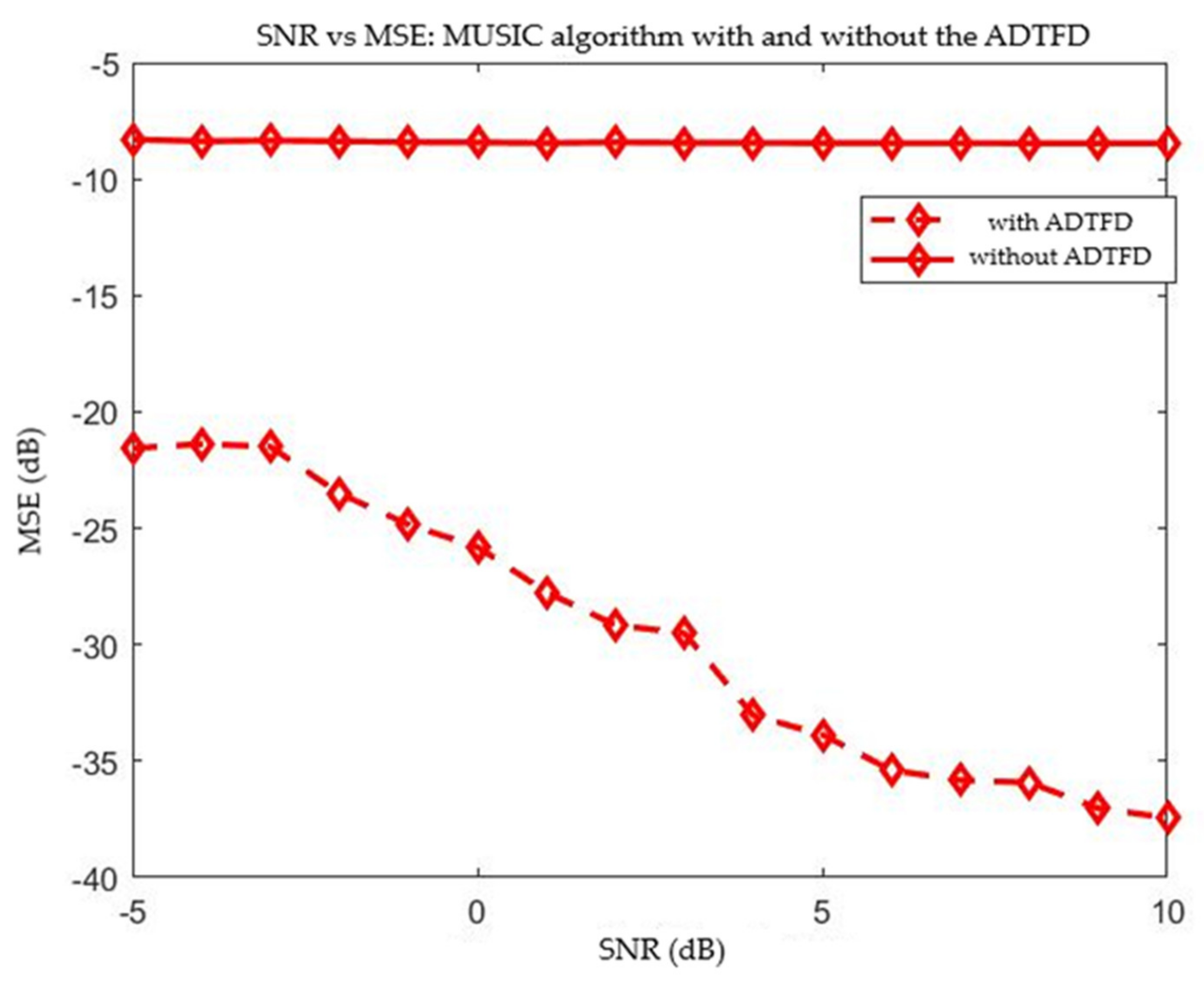
Figure 8.
SNR vs. MSE plot of the ESPRIT algorithm with and without ADTFD (solid line and the dashed line represents the cases without ADTFT and with ADTFD, respectively).
Figure 8.
SNR vs. MSE plot of the ESPRIT algorithm with and without ADTFD (solid line and the dashed line represents the cases without ADTFT and with ADTFD, respectively).

Figure 9.
SNR vs. MSE plot of the EVD algorithm with and without ADTFD (solid line and the dashed line represent the cases without ADTFT and ADTFD, respectively).
Figure 9.
SNR vs. MSE plot of the EVD algorithm with and without ADTFD (solid line and the dashed line represent the cases without ADTFT and ADTFD, respectively).

Table 1.
DOA estimation results without using the ADTFD algorithm.
| DOA Estimation without ADTFD Algorithm | ||||||||||||
|---|---|---|---|---|---|---|---|---|---|---|---|---|
| SNR (dB) | MUSIC | ESPRIT | EVD | |||||||||
| T1 | T2 | T3 | T4 | T1 | T2 | T3 | T4 | T1 | T2 | T3 | T4 | |
| −5 dB | 35 | 35 | 35 | 35 | 0 | 2 | 74 | 0 | 13 | 32 | 40 | 67 |
| 0 dB | 36 | 36 | 36 | 36 | 0 | 9 | 58 | 0 | 18 | 22 | 43 | 58 |
| 5 dB | 37 | 37 | 37 | 37 | 0 | 14 | 49 | 0 | 6 | 31 | 39 | 79 |
| 10 dB | 37 | 37 | 37 | 37 | 0 | 14 | 49 | 0 | 12 | 45 | 45 | 83 |
Table 2.
DOA estimation results using the ADTFD algorithm.
| DOA Estimation with ADTFD Algorithm | ||||||||||||
|---|---|---|---|---|---|---|---|---|---|---|---|---|
| SNR (dB) | MUSIC | ESPRIT | EVD | |||||||||
| T1 | T2 | T3 | T4 | T1 | T2 | T3 | T4 | T1 | T2 | T3 | T4 | |
| −5 dB | 18 | 30 | 50 | 58 | 0 | 8 | 59 | 0 | 15 | 39 | 41 | 62 |
| 0 dB | 16 | 34 | 43 | 57 | 0 | 10 | 56 | 0 | 17 | 32 | 49 | 66 |
| 5 dB | 16 | 29 | 42 | 59 | 0 | 18 | 44 | 0 | 19 | 54 | 31 | 41 |
| 10 dB | 16 | 30 | 44 | 61 | 0 | 9 | 57 | 0 | 3 | 28 | 32 | 48 |
Table 3.
Computation time for the DOA estimation algorithms.
| Method | Without ADTFD | With ADTFD |
|---|---|---|
| MUSIC | 0.30 s | 1.83 s |
| ESPRIT | 0.10 s | 1.54 s |
| Eigenvalue decomposition | 0.21 s | 1.66 s |
Publisher’s Note: MDPI stays neutral with regard to jurisdictional claims in published maps and institutional affiliations. |
© 2022 by the authors. Licensee MDPI, Basel, Switzerland. This article is an open access article distributed under the terms and conditions of the Creative Commons Attribution (CC BY) license (https://creativecommons.org/licenses/by/4.0/).
Share and Cite
MDPI and ACS Style
Eranti, P.K.; Barkana, B.D. An Overview of Direction-of-Arrival Estimation Methods Using Adaptive Directional Time-Frequency Distributions. Electronics 2022, 11, 1321. https://doi.org/10.3390/electronics11091321
AMA Style
Eranti PK, Barkana BD. An Overview of Direction-of-Arrival Estimation Methods Using Adaptive Directional Time-Frequency Distributions. Electronics. 2022; 11(9):1321. https://doi.org/10.3390/electronics11091321
Chicago/Turabian StyleEranti, Pranav Kumar, and Buket D. Barkana. 2022. "An Overview of Direction-of-Arrival Estimation Methods Using Adaptive Directional Time-Frequency Distributions" Electronics 11, no. 9: 1321. https://doi.org/10.3390/electronics11091321
Note that from the first issue of 2016, this journal uses article numbers instead of page numbers. See further details here.