Article

Transfer Learning-Based Automatic Hurricane Damage Detection Using Satellite Images

1
Chitkara University Institute of Engineering and Technology, Chitkara University, Punjab 140401, India
2
Department of Electronics and Communication Engineering, University Institute of Technology, Himachal Pradesh University, Shimla 171005, India
3
Faculty of Computer Science, Ho Chi Minh City Open University, Ho Chi Minh City 70000, Vietnam
4
College of Computer Science and Information Systems, Najran University, Najran 61441, Saudi Arabia
*
Author to whom correspondence should be addressed.
Electronics 2022, 11(9), 1448; https://doi.org/10.3390/electronics11091448
Submission received: 4 April 2022 / Revised: 28 April 2022 / Accepted: 28 April 2022 / Published: 30 April 2022
(This article belongs to the Section Computer Science & Engineering)

Abstract

:
After the occurrence of a hurricane, assessing damage is extremely important for the emergency managers so that relief aid could be provided to afflicted people. One method of assessing the damage is to determine the damaged and the undamaged buildings post-hurricane. Normally, damage assessment is performed by conducting ground surveys, which are time-consuming and involve immense effort. In this paper, transfer learning techniques have been used for determining damaged and undamaged buildings in post-hurricane satellite images. Four different transfer learning techniques, which include VGG16, MobileNetV2, InceptionV3 and DenseNet121, have been applied to 23,000 Hurricane Harvey satellite images, which occurred in the Texas region. A comparative analysis of these models has been performed on the basis of the number of epochs and the optimizers used. The performance of the VGG16 pre-trained model was better than the other models and achieved an accuracy of 0.75, precision of 0.74, recall of 0.95 and F1-score of 0.83 when the Adam optimizer was used. When the comparison of the best performing models was performed in terms of various optimizers, VGG16 produced the best accuracy of 0.78 for the RMSprop optimizer.

1. Introduction

There has been a steady increase in the occurrence of natural disasters since 1980 globally. The number of people that are prone to disasters is also increasing [1]. Amongst natural disasters, the most catastrophic disaster includes hurricanes that occur in areas with warm seawaters that are in tropical and subtropical areas. The sun heats seawater, leading to the formation of enormous clouds, which cause excessive rainfall, floods and very fast-moving winds [2]. Damage of approximately USD 265 billion was estimated in the US in the year 2017 due to three major hurricanes (Harvey, Maria and Irma). These hurricanes affected thousands of people and caused many fatalities. During such difficult times, the affected people required assistance. Hence, it is very essential assess the destruction brought about due to hurricanes [1].
Satellite images have been used to determine whether there has been damage inflicted by the hurricane or not. Satellite images have been gaining immense popularity for monitoring hurricanes. Ground surveys are time-consuming and also labor-intensive [3].
In artificial intelligence, transfer learning is a technique that involves reusing an already trained model on a different but related problem. This technique is now being popularly used in deep learning when the dataset is not large. This technique helps in the reduction in resources and the labeled data required for training newer models. It helps reduce training times [4].
A convolutional neural network consists of feature extraction as the first stage and classification as the final stage. In transfer learning, the classification stage is altered. The initialization of the network has been performed with weights from the ImageNet dataset [4]. The convolutional layers and the max-pooling layers are frozen so that no modification of weights takes place. Only the dense or the fully connected layers are left free to be altered. After this, the retraining of the model is performed. The advantage of the feature extraction stage is taken, and only the final classifier is tuned, which works better with smaller datasets. This is the reason for why it is called transfer learning, as the advantage of the knowledge of one problem can solve the second problem [5].
This paper involves the study of hurricane damage detection using satellite images. The estimation of the intensity of hurricanes was performed by using deep convolutional neural networks. Infrared images were used for estimation and were obtained from the satellite source. The adopted method is known as Deep Phurie, and it produced a very low root mean square (RMS) value in comparison with the method adopted earlier, which is known as Phurie. Deep Phurie is completely automatic, but this paper does not evaluate the damage post-disaster [2]. Furthermore, deep convolutional neural networks were used to estimate of the intensity of the tropical cyclones or hurricanes that took place over a period from 1998 to 2012. Regularization techniques were used along with many convolutional and dense layers. This technique helped in extracting features from hurricane images effectively. A low RMS value and an improved accuracy were obtained [6]. However, these data were noisy and not of good quality.
A multilayer perceptron was proposed for the determination of the connection between the appearance of hurricanes and the high-energy particles that flow out from the sun. A multilayer perceptron is an artificial neural network accompanied by backpropagation. It was found that hurricane appearances could take place a few days before the breakout of a solar wind [7].
As a deep learning method, a single-shot multibox detector (SSD) was employed for the calculate of the destruction inflicted on buildings due to hurricane Sandy, which occurred in the year 2012. The Vgg16 model and the SSD model were used, and improvements of 72% and 20% in mAp and mF1, respectively, were observed [8]. The CNN model was used to determine areas that were severely affected by Hurricane Harvey. Satellite images were used for the extraction of man-made features such as roads and buildings before and after the occurrence of the disaster. An F1 score of 81.2% was achieved [9].
Damage assessment after a hurricane is of utmost importance. In this paper, the author created a benchmark dataset for the property that became damaged by Hurricane Harvey. The dataset consisted of both undamaged and impaired building images, and they were obtained from satellite imagery. FEMA and TOMNOD were the sources of this dataset [10].
The destruction brought about because of hurricane Dorian has been determined using satellite imagery and artificial intelligence. The austerity of the destruction caused due to the hurricanes has been determined, and an accuracy of 61% was achieved [11].
Earlier studies focused on finding the intensity of hurricanes and providing a benchmark dataset for damage detection. Fewer studies have focused on classifying hurricane images into damaged and undamaged classes. In this paper, a comparative analysis of the four transfer learning models that include DenseNet121 [12], VGG16 [13], MobileNetV2 [14] and InceptionV3 [15] has been performed with respect to confusion matrix parameters. These models have also been used for determining the destruction brought about on buildings because of Hurricane Harvey.
The objectives of this study include the following:
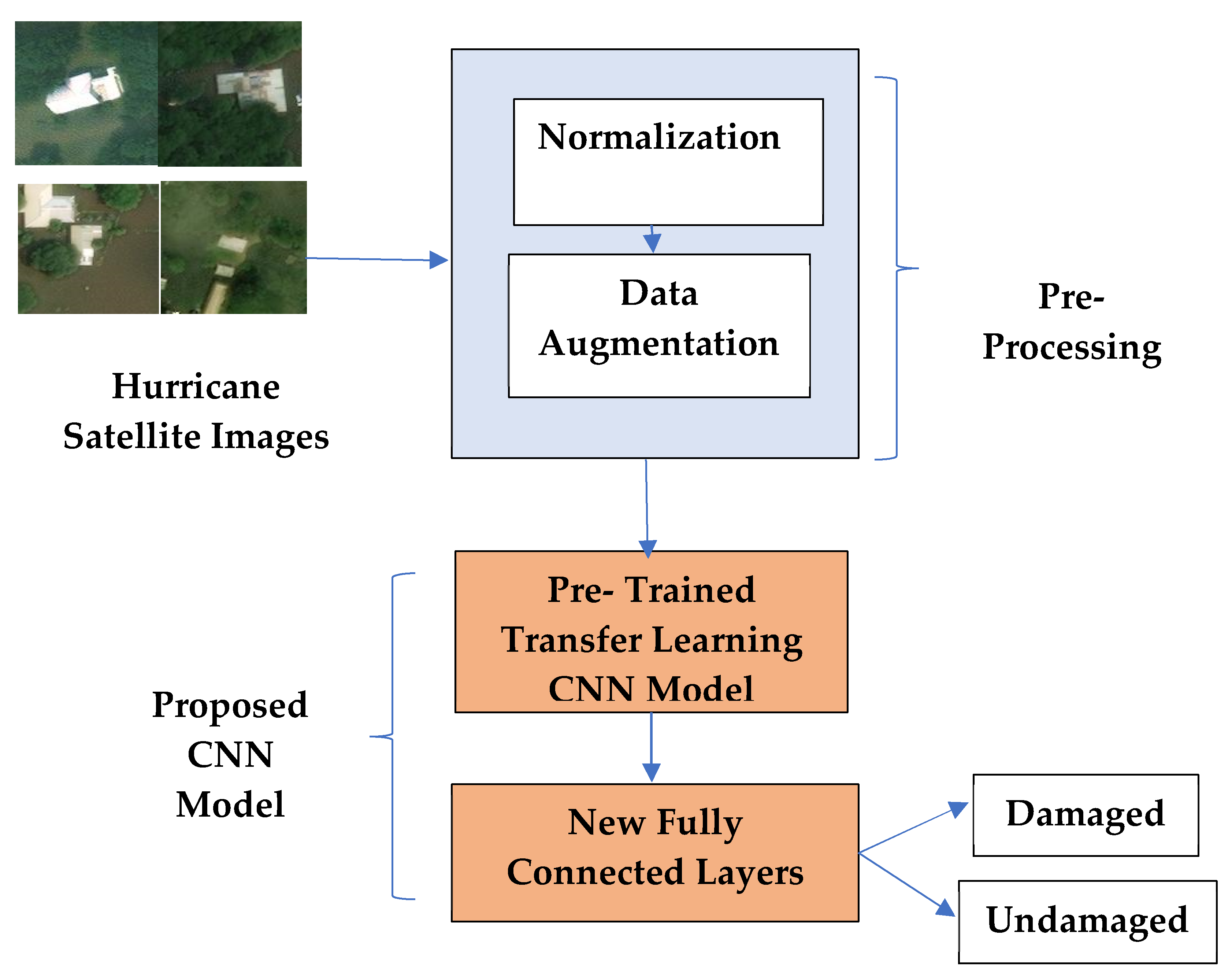
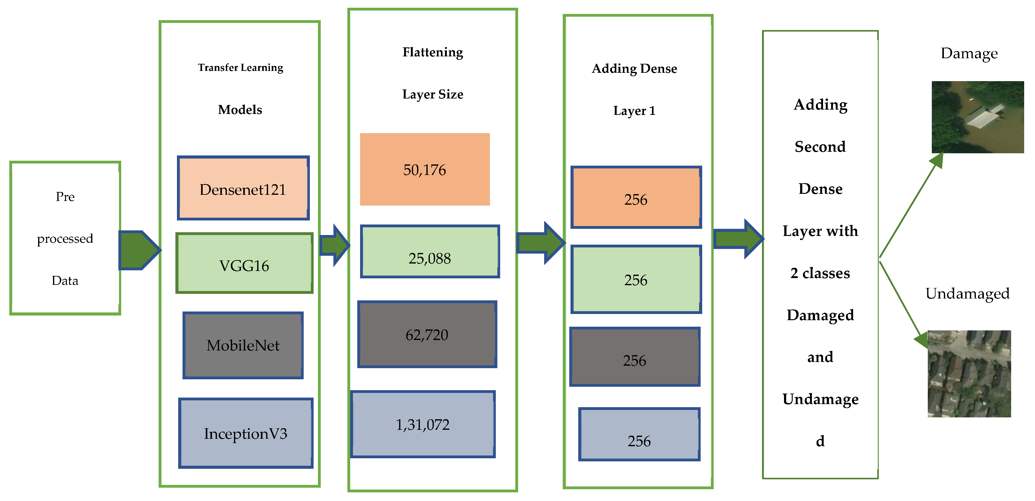
  • Addition of a newer set of layers to the pre-trained models for classification of the satellite images of hurricanes into damaged and undamaged categories;
  • To generalize the model by applying data augmentation techniques to images;
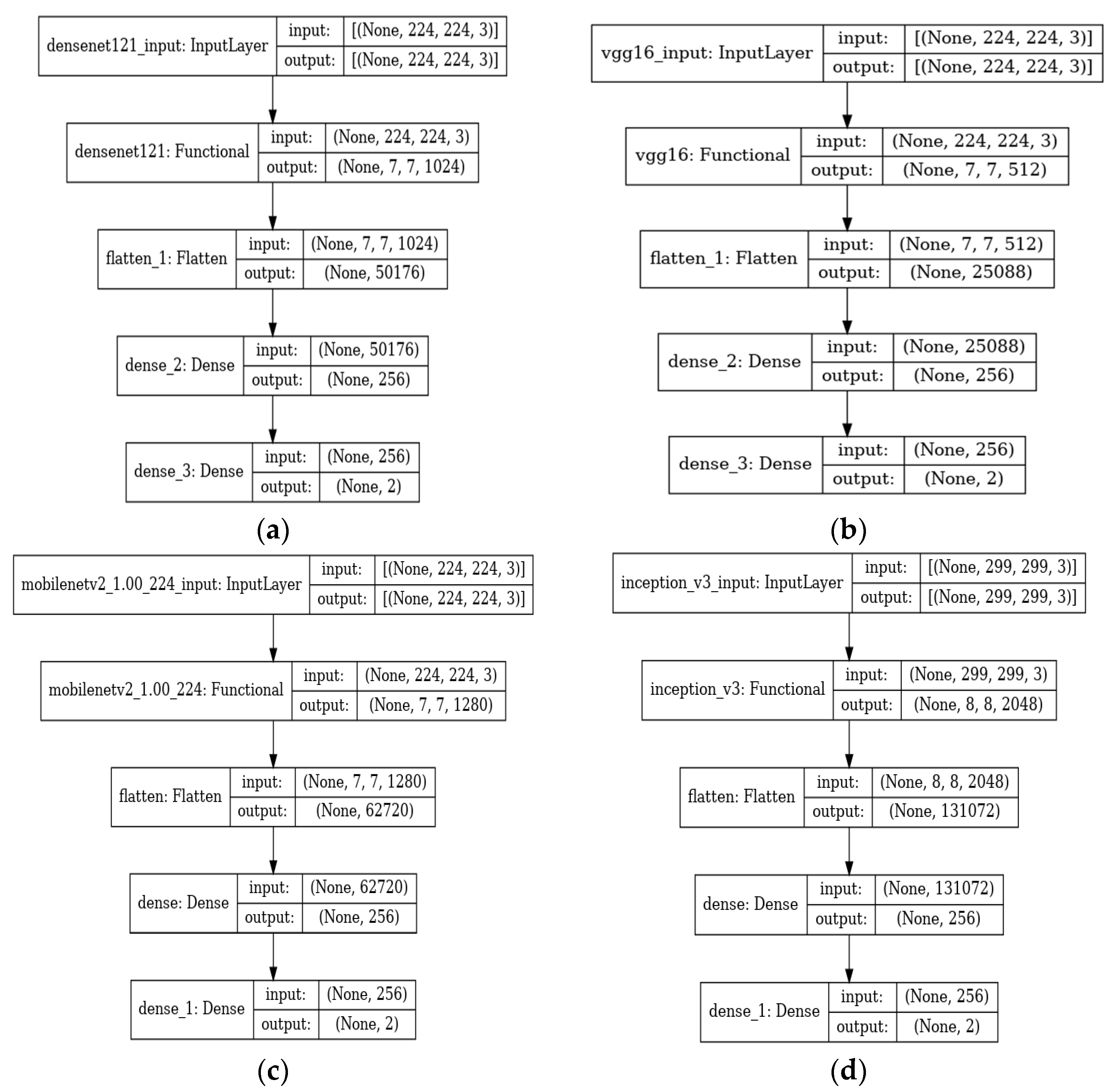
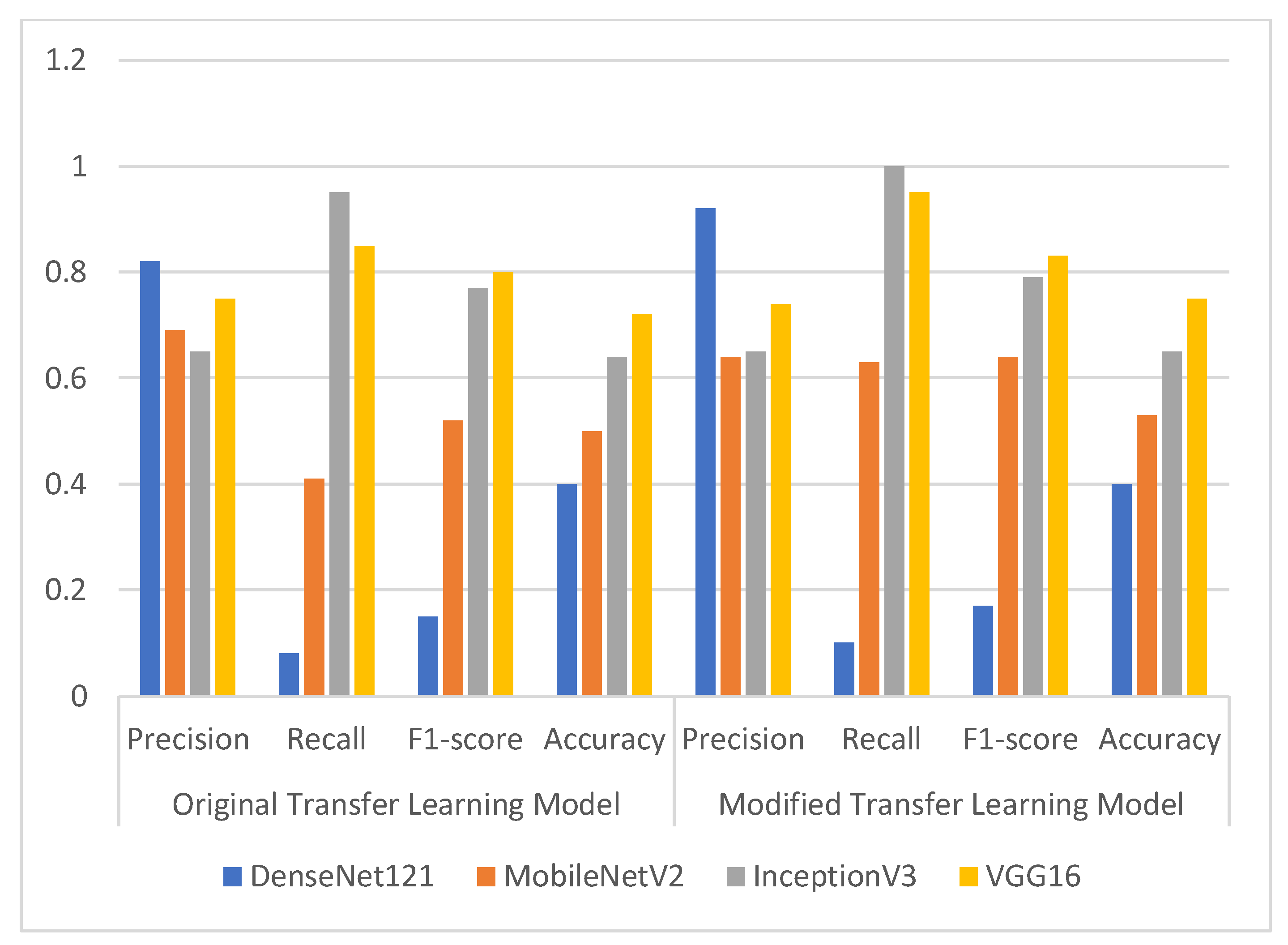
  • To perform a comparative study based on accuracy, precision, recall and F1-score for the four pre-trained models, which include VGG16, MobileNetV2, InceptionV3 and DenseNet121, at a learning rate of 0.0001 and 40 epochs.
  • To compare the best performing models for various optimizers, which include SGD, Adadelta, Adam and RMSprop.
The rest of the paper is organized as follows: proposed methodology in Section 2; results and discussion in Section 3; conclusion and future scopes in Section 4.

2. Proposed Methodology

The model that has been presented for automatic damage detection due to hurricanes is shown in Figure 1. The platform used to create and run the algorithm is Kaggle. The model classifies satellite images into damaged and undamaged categories. The methodology comprises two main steps: The first is preprocessing [16,17], which is further divided into normalization and data augmentation, and the second is classification using the pre-trained CNN models. Each stage has been described below.

2.1. Preprocessing

The satellite images of the Houston region used in this study were captured by optical sensors. The images could be covered with clouds either partially or fully. This implies that the images obtained from the satellites have been corrupted by noise. The nature of the noise is unknown, meaning that it could be a result of fluctuations in light, the sensor of the camera or artifacts. Improving the quality of the images so that good results can be obtained is imperative. For this purpose, a denoising operation needs to be performed, which could be based on wavelets [18] or can be acquired from a compressive sensing method [19].
For the suppression of unwanted distortions or enhancement of some of the features of the images, pre-processing steps such as resizing were used. The original size of the satellite images of hurricanes is 128 × 128. The resizing of the satellite images of the hurricane was performed. The resizing of the images was performed at 224 × 224 when Vgg16, MobileNetV2 and DenseNet121 transfer learning techniques were applied. The images were resized to 299 × 299 on the application of the InceptionV3 technique.
The two main steps of the preprocessing stage, which include normalization and data augmentation, have also been explained in this section.

2.1.1. Normalization

Normalization is a very important step for maintaining numerical stability in a model. Normalization helps in learning faster and brings about stability in gradient descents. The input image pixels have, thus, been normalized in the values between 0 and 1. Normalization is brought about by multiplying pixel values by 1/255.

2.1.2. Data Augmentation

The augmentation of data is a technique utilized to generalize the model by applying random transformations with respect to input images [20,21]. It increases the variability and robustness of the model as the model becomes new and modified versions of the input data. An image data generator is utilized for augmenting the data, which is an on-the-fly data augmentation method because augmentation is performed during training time. The image data generator returns only the randomly modified images and not the original images. Data augmentation has been applied only to training images and not to testing images.
The techniques adopted for data augmentation in this study are rotation, width shifting, height shifting, horizontal flipping and zoom operation.

2.2. Hurricane Damage Detection Using Pre-Trained CNN Models

In this paper, four pre-trained models, which include VGG16 [22], MobileNetV2 [23], InceptionV3 [24] and DenseNet121 [25], have been used for classifying satellite images into damaged and undamaged classes.
Transfer learning models are models trained on very large datasets that include millions of images. As the models have been trained on such a large dataset, a generalization of the model takes place. The features that have been learned from the larger datasets help in solving a different problem consisting of lesser data or a smaller dataset. This helps eliminate the need to train a model from scratch.
The description of the architectures of these models is shown in Table 1.
The VGG16 model comprises 16 layers that have weights and has approximately 138 million parameters. There are 13 convolutional layers and 3 fully connected layers. The VGG16 model is widely used because of its ease of implementation [22]. MobileNetV2 consists of 53 layers and 3.4 million parameters. It has been derived from the MobileNetV1 model, which utilizes depth-wise convolution as the building block of the model. However, the additional feature from the previous models is that it has an additional inverted residual layer [23]. This model is used because it is smaller in size and also cost-effective. There are nineteen bottleneck layers that were residual. There are 42 layers in the InceptionV3 model and 24 million parameters. InceptionV3 is an advanced version of InceptionV2. It reduces the amount of computations as it uses factorization methods [24]. For InceptionV3, the input image size is (299, 299, 3). Densenet121 consists of 121 layers with trainable weights. DenseNet121 has 8 million parameters. In this model, the network proceeds deeper as each layer is connected to all the other layers; for example, the first layer is connected to the second, third, fourth and so on layers. This leads to a improved maximum flow of information amongst the layers [25].

2.3. Tuning the Hyper-Parameters

The training of the four models has been performed for 40 epochs and a batch size of 100. The total epochs refer to how often the learning algorithm will be working through the complete dataset. Batch size refers to the number of training examples that would be utilized in a single iteration [26]. A batch size of 100 implies that 100 samples from the training dataset would be used for the estimation of the error gradient before the weights of the models are updated. The learning rate (LR) is another important hyperparameter that should not be either too big or too small [27]. It is used for finding the learning speed of the proposed models. The model would take a lot more time to reach the minimum loss if the LR is too small and if the LR is too high due to the fact that overshooting the low loss areas can take place. A learning rate of 0.0001 has been chosen in this paper. The batch size, number of epochs [28] and the learning rate have all been decided empirically.
Furthermore, the activation function [29] used is a rectified linear unit (ReLU) [30]. The fully connected head, used along with all the four pre-trained models, is shown in Figure 2. The pre-trained block is followed by a flattening layer and two dense layers. The flattening layer size of the DenseNet121 model is 50,176; for VGG16, the size is 25,088. For the MobileNetV2 model, the flattening layer size is 62,720; for InceptionV3, the size is 131,072. After the flattening layer, a dense layer of size 256 is applied. Finally, a dense layer with two classes that is damaged and undamaged is used.
The block diagram of the four pre-trained models, which include DenseNet121, VGG16, MobileNetV2 and InceptionV3, is displayed in Figure 3.
The block diagram of DenseNet121 is shown in Figure 3a. The input is of 224 × 224 × 3 sizes. This is applied to the DenseNet121 model, and the output obtained is of 7 × 7 × 1024 size. This is then applied to the new fully connected head, which comprises the flattening and dense layers. The output of the flattening layer is of 50,176 in size. The output of the first dense layer is 256, and the last dense layer classifies the images into two classes, which include damaged and undamaged classes.
The block diagram of the VGG16 model is demonstrated in Figure 3b. An input size of 224 × 224 × 3 was applied to the model, and an output of 7 × 7 × 512 was obtained. The output of the flattening layer is 25,088, and the outputs of the dense layers are 256 and 2 in size.
The block diagram of MobileNetV2 has been demonstrated in Figure 3c, for which its input image size is 224 × 224 × 3. This is applied to the model and an output of 7 × 7 × 1280 is obtained. The output after the application of the flattening layer is 62,720, and the outputs of the two dense layers are 256 and 2, respectively.
Figure 3d presents the InceptionV3 model, for which its input image size is 299 × 299 × 3. The output when this input is applied to the model is 8 × 8 × 2048. The output obtained after the flattening layer is of size 131,072.

3. Results and Discussion

This section includes the results performed on the four pre-trained models that are DenseNet121, VGG16, MobileNetV2 and InceptionV3, considering various parameters and then comparing the results of all four models.

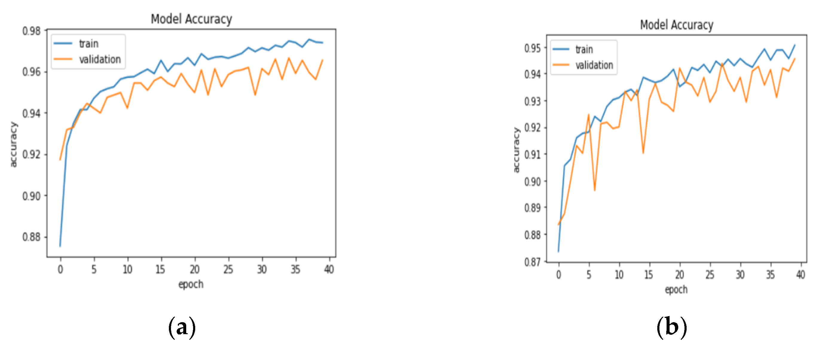
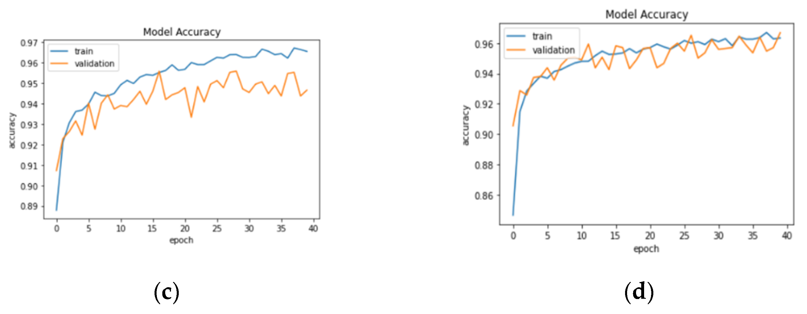
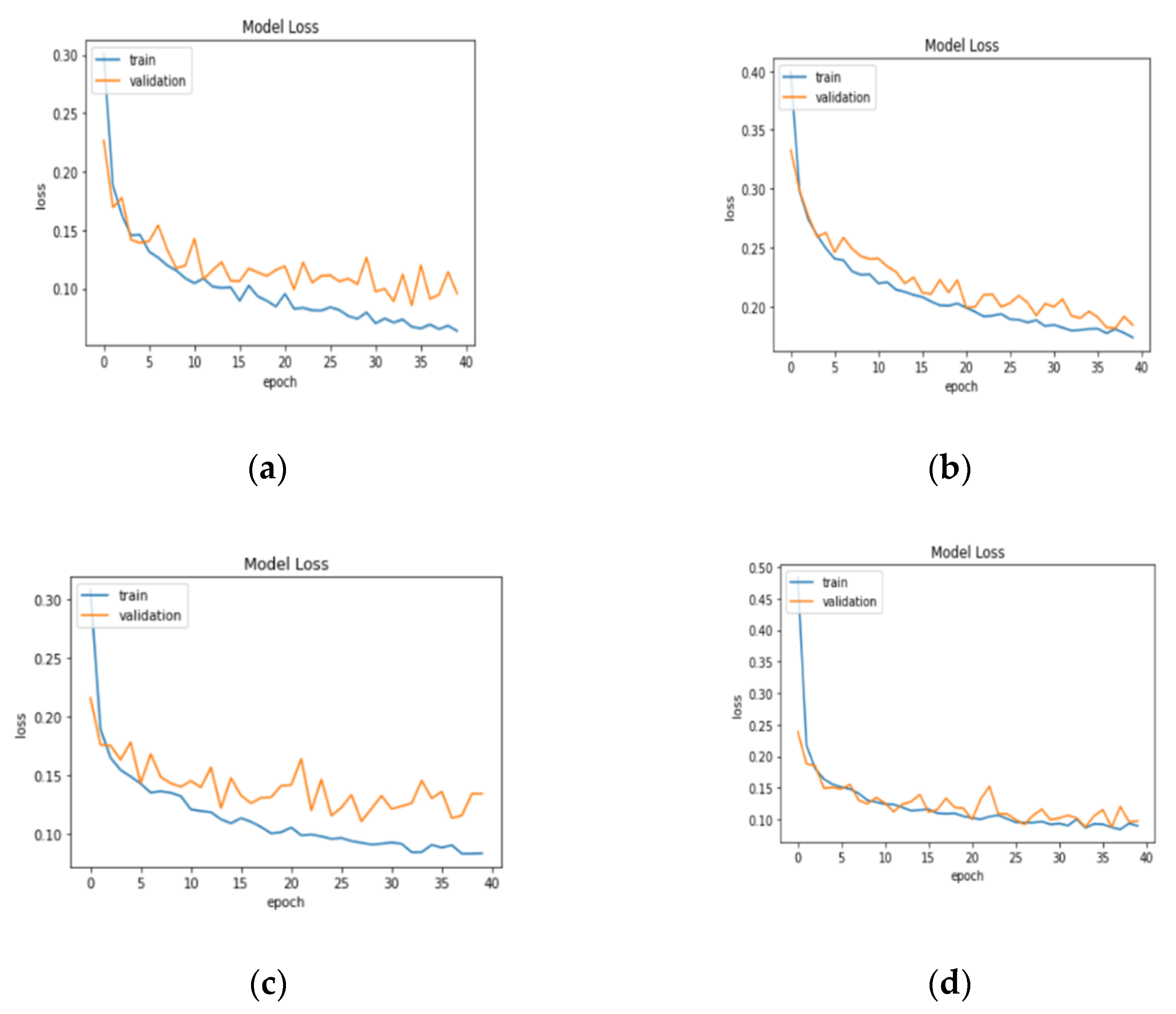
3.1. Result Analysis in Terms of Loss and Accuracy

The results of the four transfer learning models, which include DenseNet121, VGG16, MobileNetV2 and InceptionV3, in terms of training performance parameters are shown in Table 2. Training loss, training accuracy, training recall, validation loss, validation accuracy, and validation recall values for the models have been shown for various epochs in Table 2.
As per Table 2, the highest training accuracy of 0.9727 and training recall of 0.9735 were obtained by the DenseNet121model at the 40th epoch and learning rate of 0.0001. The highest validation accuracy of 0.9670 and validation recall of 0.9658 were obtained by the InceptionV3 model at the 40th epoch. The lowest training loss of 0.0666 and validation loss of 0.0956 has been obtained by the DenseNet121 model at the 40th epoch.
The training and validation accuracies for all the proposed models are demonstrated in Figure 4. The model accuracy for the DenseNet121 model has been displayed in Figure 4a. The model accuracy for the VGG16 model has been shown in Figure 4b; Figure 4c demonstrates the model’s accuracy for the MobileNetV2 model, and Figure 4d demonstrates the model accuracy for the InceptionV3 model.
Figure 5 demonstrates the training and validation loss for all four models. Figure 5a shows the model loss for DenseNet121, Figure 5b shows the model loss for the VGG16 model, Figure 5c shows the model loss for the MobileNetV2 model and Figure 5d displays the model loss for InceptionV3.

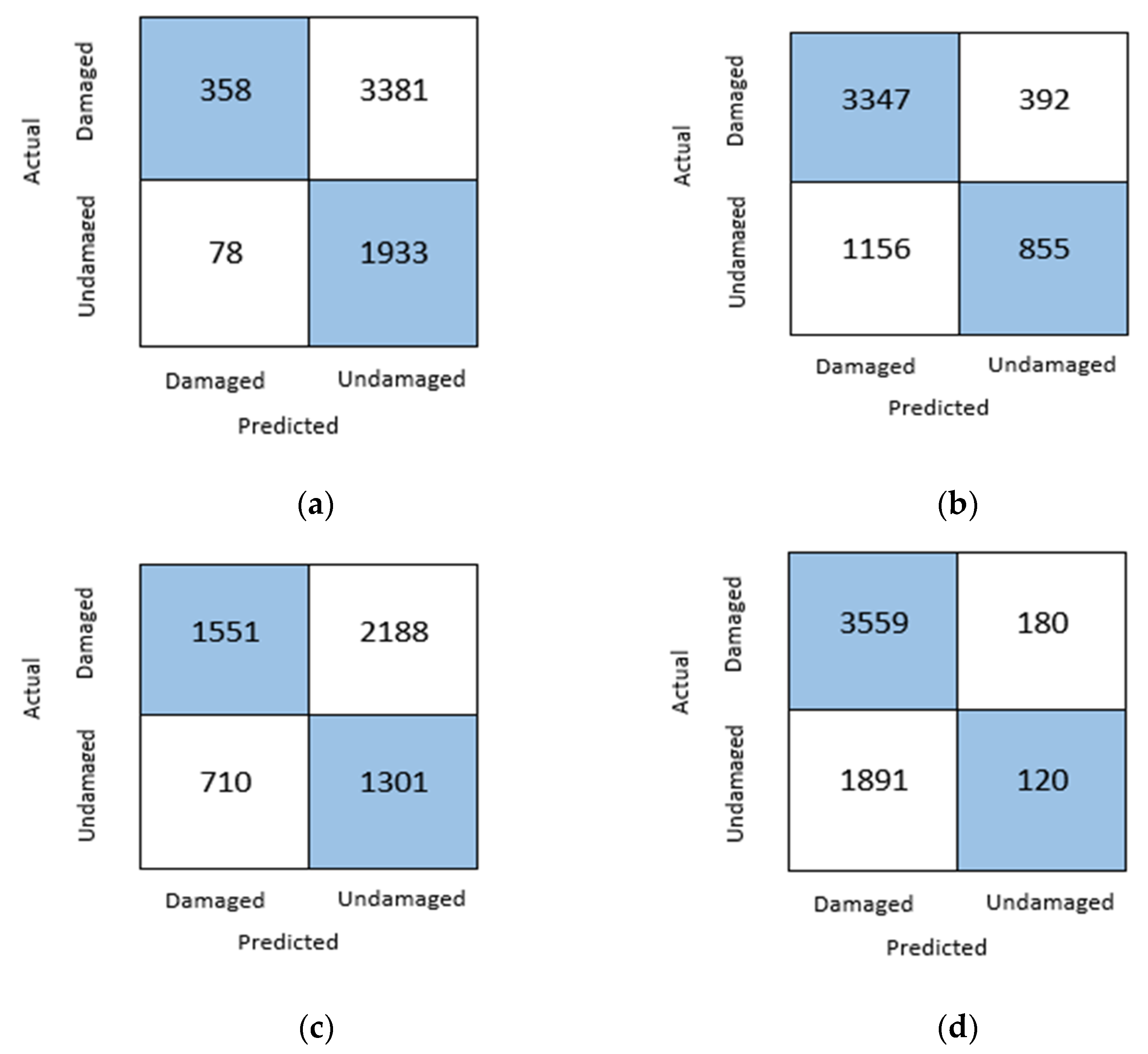
3.2. Confusion Matrix Parameter Result Analysis

Figure 6 shows the confusion matrix for all four models, which include DenseNet121, VGG16, MobileNetV2 and InceptionV3. The confusion matrix parameters are accuracy, precision, recall and F1-score [31,32], and they can be calculated with the help of the confusion matrix.
The results of the classification report or the confusion matrix parameters of the four original and modified models in terms of precision, recall, F1-score and accuracy have been displayed in Table 3. From Table 3, it is concluded that the best precision of 0.92 is obtained by the modified DenseNet121 model as compared to the 0.82 precision obtained by the original DenseNet121 model. The best recall of 1.00 is obtained by the modified InceptionV3 model. The best F1-score of 0.83 and accuracy of 0.75 are obtained by the modified VGG16 model. An improvement in the recall is 0.95, and it is obtained by the modified VGG16 model as compared to the recall of 0.85 obtained by the original VGG16 model.
Figure 7 compares the original and modified models in terms of the classification report parameters, which include precision, recall, F1-score and accuracy. The best accuracy of 0.75 is obtained by the VGG16 model followed by an accuracy of 0.65 obtained by the InceptionV3 model. The highest F1 score of 0.83 is obtained by the VGG16 model. The highest recall of 1.00 was obtained from the InceptionV3 model followed by a recall of 0.95 in the VGG16 model.

3.3. Comparison of Results of Various Optimizers

Different optimizers, which include SGD [33], Adadelta [34], Adam [35] and RMSprop [36], have been compared for the two best performing models, which include VGG16 and InceptionV3, as shown in Table 4 and Table 5 and Figure 8 and Figure 9.

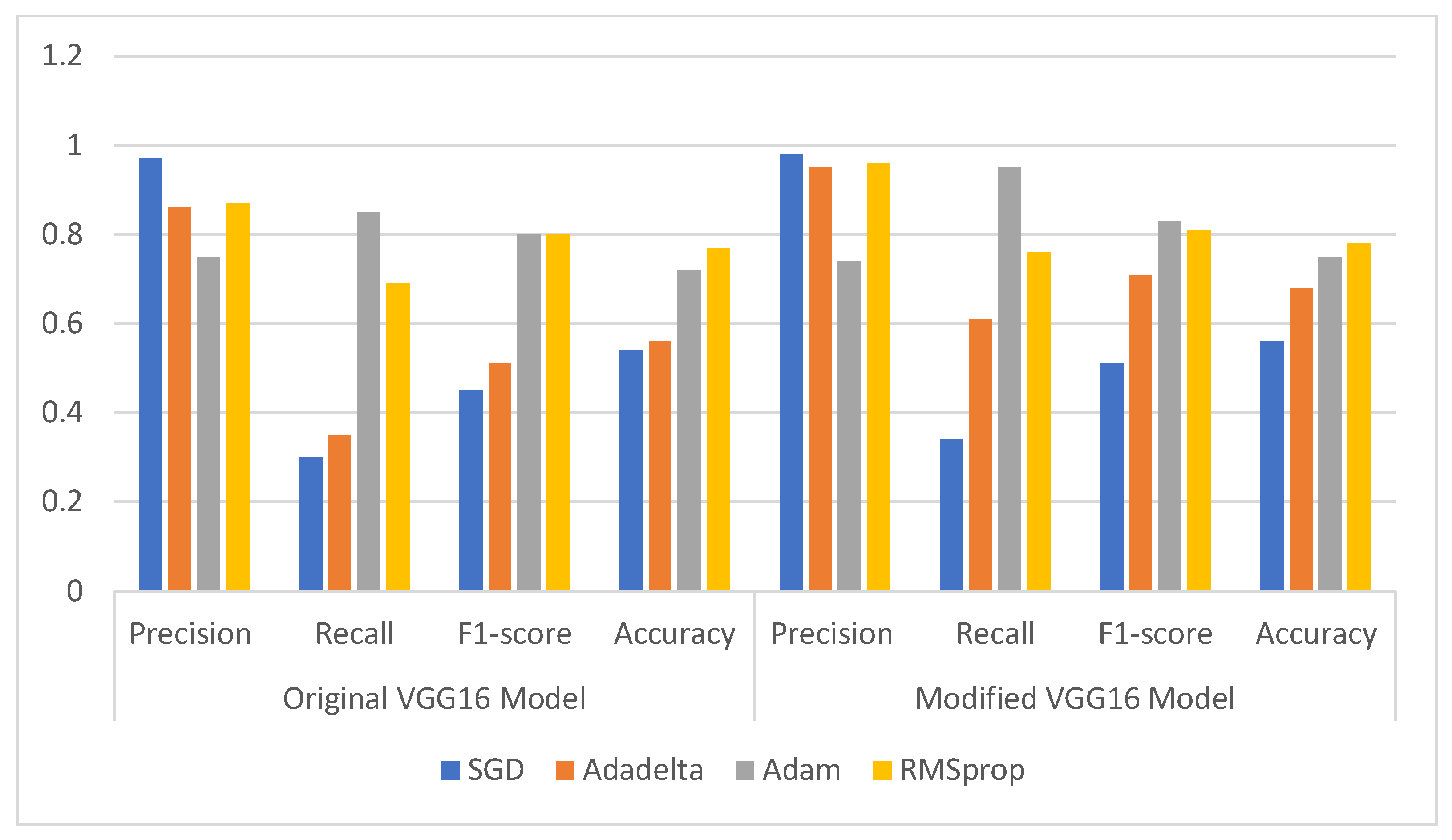
3.3.1. Comparison of Original and Modified VGG16 Model

Table 4 shows the comparison of the original and modified VGG16 model for the four optimizers, which include SGD, Adadelta, Adam and RMSprop. The highest precision of 0.98 is obtained for the modified VGG16 model for the SGD optimizer. The highest recall of 0.95 is obtained by the modified model for the Adam optimizer. An improved F1-score of 0.83 is obtained for the Adam optimizer. The highest accuracy of 0.78 is obtained by the RMSprop optimizer.
Figure 8 displays the comparison of the original and modified VGG16 model. There is an improvement in accuracy from 0.77 for the original model to 0.78 for the modified model. An improved F1-score of 0.83 is obtained by the modified VGG16 model. The highest recall of 0.95 and precision of 0.98 were obtained by the modified model.

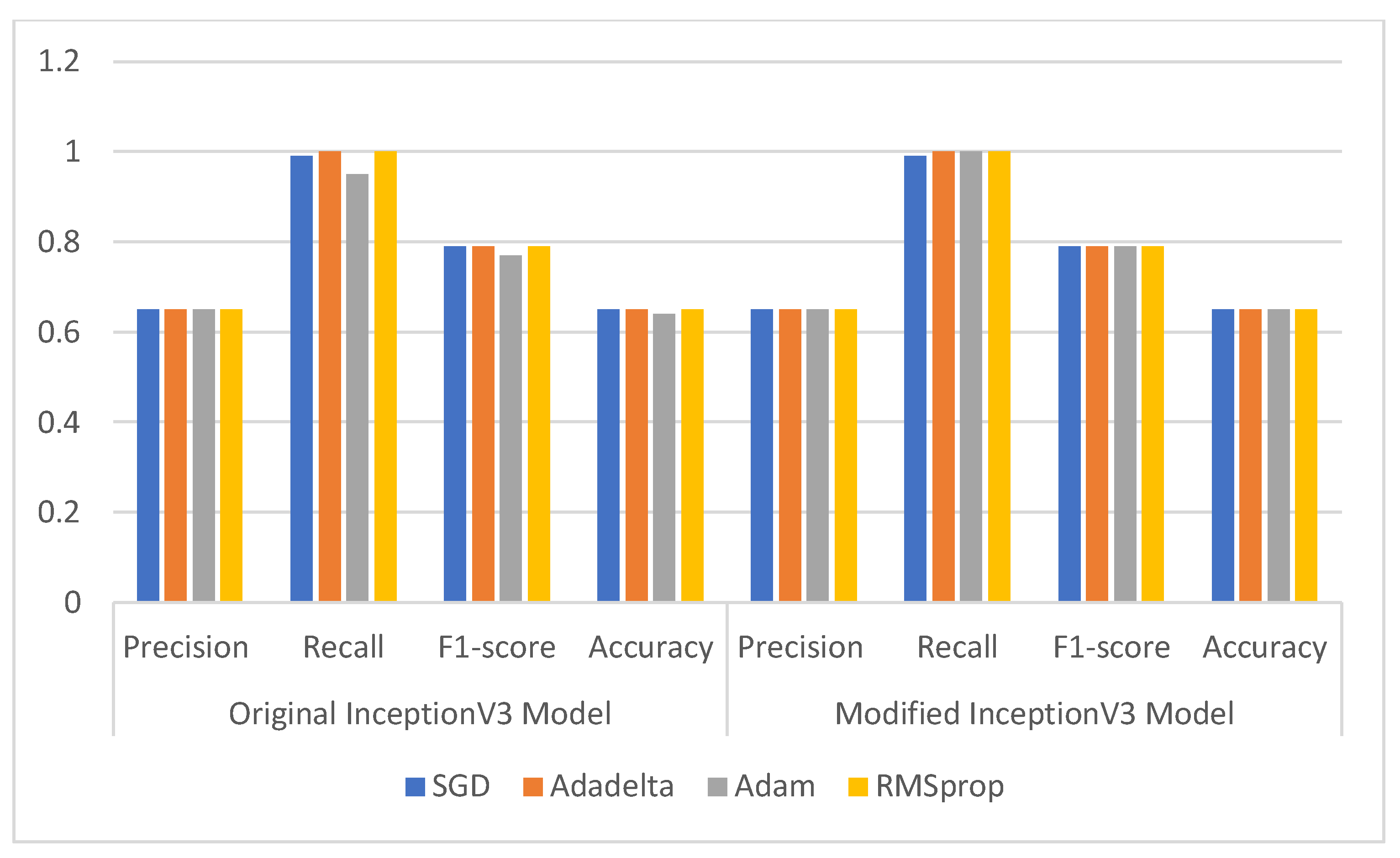
3.3.2. Comparison of Original and Modified InceptionV3 Model

Table 5 presents the comparison of the original and modified InceptionV3 model for four optimizers. It can be inferred from the table that, in the case of the InceptionV3 model, all optimizers produced almost the same results in terms of precision, F1-score and accuracy. For the modified model, an equal precision of 0.65, F1-score of 0.79 and accuracy of 0.65 were obtained for all four optimizers.
Figure 9 compares the results of the original and the modified InceptionV3 model, and it was observed that almost the same results were obtained for the model for all four optimizers.

3.4. Classification and Misclassification Results

Figure 10 shows the classification and misclassification results for the VGG16 model. Figure 10a shows that the actual class is undamaged and the predicted class is also undamaged. Figure 10b shows that the actual class is damaged and the predicted class is also damaged.
Figure 10c,d display the misclassification results. For Figure 10c, the actual class is undamaged and the predicted class is damaged. For Figure 10d, the actual class is damaged and the predicted class is undamaged.

3.5. Comparison with Present State-of-Art Deep Learning Models

Table 6 presents the comparison of the best Transfer learning model (VGG 16) obtained in this paper with the state-of-the-art deep learning models. The study was performed on 23,000 satellite images of the hurricane. VGG16 obtained an accuracy of 78%, which is more than the other deep learning models presented in Table 6. In reference number [37], work was performed on 1128 hurricane images using a VGG16 model and an accuracy of 64.61% was obtained. A stacked CNN model was used in reference number [11], and an accuracy of 61% was obtained. Work on 61,000 hurricane images was performed in reference [38] using a VGG16 model, and an accuracy of 74% was achieved. Accuracy at 77.85% was obtained by the CNN model comprising five convolutional layers in reference [6]. The hurricane images used were 48,828 in number.

3.6. Comparison with Present State-of-Art Machine Learning Models

This section compares the best Transfer learning model (VGG16) obtained in this paper with commonly used machine learning algorithms. VGG16 achieved an accuracy of 78%, and the best accuracy was achieved with the RMSProp optimizer and 23,000 satellite images. The hurricanes are accompanied by floods. Most authors have worked on floods using machine learning algorithms. Naive Bayes achieved an accuracy of 78.51% and Support Vector Machine achieved an accuracy of 91% when applied to 7500 images [39]. Random forest attained an accuracy of 82% when applied to 201 images [40]. Random forest attained an accuracy of 92% on 255 flood images [41]. The machine learning results are better since the analysis has been conducted on lower numbers of images, whereas the deep learning transfer learning models proposed in this paper have worked on a greater number of images, which involved 23,000 images.

4. Conclusions and Future Scope

In this paper, four pre-trained models, includingDenseNet121, VGG16, MobileNetV2 and InceptionV3, based on transfer learning have been put forward for the detection of destruction inflicted on buildings due to Hurricane Harvey, which took place in the Greater Houston region in the year 2017. The comparison of the four models has been performed based on training accuracy, training recall, training loss, validation accuracy, validation recall and validation loss. The highest training accuracy of 0.9727 and training recall of 0.9735 was obtained by the DenseNet121model at the 40th epoch and learning rate of 0.0001. The highest validation accuracy of 0.9670 and validation recall of 0.9658 was obtained by the InceptionV3 model at the 40th epoch. The lowest training loss of 0.0666 and validation loss of 0.0956 was obtained by the DenseNet121 model at the 40th epoch.
A comparison was also performed in terms of the classification report’s parameters, and it was found that VGG16 outperformed other models by obtaining an accuracy of 0.75, an F1 score of 0.83 and a recall of 0.95.
When the comparison was performed for the best-performing models for various optimizers in terms of the classification report parameters, it was found that VGG16 performed better by obtaining an accuracy of 0.78 for the RMSprop optimizer.
Furthermore, an improvement could be brought in with values of the confusion matrix parameters. Moreover, the model could be made more generalizable by including images of other hurricanes.

Author Contributions

Conceptualization and methodology, S.K., S.G. and S.S.; formal analysis, V.T.H., S.A., T.A. and A.S.; software, validation and writing—original draft, S.K., S.G. and S.S.; writing—review and editing and data curation, V.T.H., S.A., T.A. and A.S.; supervision and funding acquisition, S.S., A.S. and T.A. All authors have read and agreed to the published version of the manuscript.

Funding

The authors are thankful to the Deanship of Scientific Research at Najran University for funding this work under the Research Collaboration Funding program grant code NU/RC/SERC/11/8.

Data Availability Statement

Conflicts of Interest

The authors declare no conflict of interest.

References

  1. Pi, Y.; Nath, N.D.; Behzadan, A.H. Convolutional neural networks for object detection in aerial imagery for disaster response and recovery. Adv. Eng. Inform. 2020, 43, 101009. [Google Scholar] [CrossRef]
  2. Dawood, M.; Asif, A. Deep-PHURIE: Deep learning-based hurricane intensity estimation from infrared satellite imagery. Neural Comput. Appl. 2019, 32, 1–9. [Google Scholar] [CrossRef]
  3. Dotel, S.; Shrestha, A.; Bhusal, A.; Pathak, R.; Shakya, A.; Panday, S.P. Disaster Assessment from Satellite Imagery by Analysing Topographical Features Using Deep Learning. In Proceedings of the 2020 2nd International Conference on Image, Video and Signal Processing, Singapore, 20–22 March 2020; pp. 86–92. [Google Scholar]
  4. Ng, H.W.; Nguyen, V.D.; Vonikakis, V.; Winkler, S. Deep learning for emotion recognition on small datasets using transfer learning. In Proceedings of the 2015 ACM on international conference on multimodal interaction, Seattle, WA, USA, 9–13 November 2015; pp. 443–449. [Google Scholar]
  5. Weiss, K.; Khoshgoftaar, T.M.; Wang, D. A survey of transfer learning. J. Big Data 2016, 3, 1–40. [Google Scholar] [CrossRef] [Green Version]
  6. Pradhan, R.; Aygun, R.S.; Maskey, M.; Ramachandran, R.; Cecil, D.J. Tropical cyclone intensity estimation using a deep convolutional neural network. IEEE Trans. Image Process. 2017, 27, 692–702. [Google Scholar] [CrossRef]
  7. Resch, B.; Usländer, F.; Havas, C. Combining machine-learning topic models and spatiotemporal analysis of social media data for disaster footprint and damage assessment. Cartogr. Geogr. Inf. Sci. 2018, 45, 362–376. [Google Scholar] [CrossRef] [Green Version]
  8. Li, Y.; Hu, W.; Dong, H.; Zhang, X. Building damage detection from post-event aerial imagery using single shot multibox detector. Appl. Sci. 2019, 9, 1128. [Google Scholar] [CrossRef] [Green Version]
  9. Doshi, J.; Basu, S.; Pang, G. From satellite imagery to disaster insights. arXiv 2018, arXiv:1812.07033. [Google Scholar]
  10. Chen, S.A.; Escay, A.; Haberland, C.; Schneider, T.; Staneva, V.; Choe, Y. Benchmark dataset for automatic damaged building detection from post-hurricane remotely sensed imagery. arXiv 2018, arXiv:1812.05581. [Google Scholar]
  11. Cheng, C.S.; Behzadan, A.H.; Noshadravan, A. Deep learning for post-hurricane aerial damage assessment of buildings. Comput. Aided Civ. Infrastruct. Eng. 2021, 36, 695–710. [Google Scholar] [CrossRef]
  12. Solano-Rojas, B.; Villalón-Fonseca, R.; Marín-Raventós, G. Alzheimer’s Disease Early Detection Using a Low Cost Three-Dimensional Densenet-121 Architecture. In International Conference on Smart Homes and Health Telematics; Springer: Cham, Switzerland, 2020; pp. 3–15. [Google Scholar]
  13. Bhalla, K.; Koundal, D.; Sharma, B.; Hu, Y.C.; Zaguia, A. A Fuzzy Convolutional Neural Network for Enhancing Multi-Focus Image Fusion. J. Vis. Commun. Image Represent. 2022, 84, 103485. [Google Scholar] [CrossRef]
  14. Sandler, M.; Howard, A.; Zhu, M.; Zhmoginov, A.; Chen, L.-C. MobileNetV2: Inverted residuals and linear bottlenecks. In Proceedings of the IEEE Conference on Computer Vision and Pattern Recognition, Salt Lake City, UT, USA, 18–23 June 2018; pp. 4510–4520. [Google Scholar]
  15. Wang, C.; Chen, D.; Hao, L.; Liu, X.; Zeng, Y.; Chen, J.; Zhang, G. Pulmonary image classification based on inception-v3 transfer learning model. IEEE Access 2019, 7, 146533–146541. [Google Scholar] [CrossRef]
  16. Scannell, C.M.; Veta, M.; Villa, A.D.; Sammut, E.C.; Lee, J.; Breeuwer, M.; Chiribiri, A. Deep-learning-based preprocessing for quantitative myocardial perfusion MRI. J. Magn. Reson. Imaging 2020, 51, 1689–1696. [Google Scholar] [CrossRef] [PubMed]
  17. Zheng, X.; Wang, M.; Ordieres-Meré, J. Comparison of data preprocessing approaches for applying deep learning to human activity recognition in the context of industry 4.0. Sensors 2018, 18, 2146. [Google Scholar] [CrossRef] [PubMed] [Green Version]
  18. Ouahabi, A. A review of wavelet denoising in medical imaging. In Proceedings of the IEEE 2013 8th International Workshop on Systems, Signal Processing and Their Applications (WoSSPA), Algiers, Algeria, 12–15 May 2013; pp. 19–26. [Google Scholar]
  19. Mahdaoui, A.E.; Ouahabi, A.; Moulay, M.S. Image Denoising Using a Compressive Sensing Approach Based on Regularization Constraints. Sensors 2022, 22, 2199. [Google Scholar] [CrossRef]
  20. Kaur, S.; Gupta, S.; Singh, S.; Koundal, D.; Zaguia, A. Convolutional Neural Network based Hurricane Damage Detection using Satellite Images. Soft Comput. 2022. [Google Scholar] [CrossRef]
  21. Shorten, C.; Khoshgoftaar, T.M. A survey on image data augmentation for deep learning. J. Big Data 2019, 6, 1–48. [Google Scholar] [CrossRef]
  22. Szegedy, C.; Liu, W.; Jia, Y.; Sermanet, P.; Reed, S.; Anguelov, D.; Erhan, D.; Vanhoucke, V.; Rabinovich, A. Going deeper with convolutions. In Proceedings of the IEEE Conference on Computer Vision and Pattern Recognition, Boston, MA, USA, 7–12 June 2015; pp. 1–9. [Google Scholar]
  23. Buiu, C.; Dănăilă, V.R.; Răduţă, C.N. MobileNetV2 ensemble for cervical precancerous lesions classification. Processes 2020, 8, 595. [Google Scholar] [CrossRef]
  24. Lin, C.; Li, L.; Luo, W.; Wang, K.C.; Guo, J. Transfer learning based traffic sign recognition using inception-v3 model. Period. Polytech. Transp. Eng. 2019, 47, 242–250. [Google Scholar] [CrossRef] [Green Version]
  25. Aral, R.A.; Keskin, Ş.R.; Kaya, M.; Hacıömeroğlu, M. Classification of trashnet dataset based on deep learning models. In Proceedings of the 2018 IEEE International Conference on Big Data (Big Data), Seattle, WA, USA, 10–13 December 2018; pp. 2058–2062. [Google Scholar]
  26. He, F.; Liu, T.; Tao, D. Control batch size and learning rate to generalize well: Theoretical and empirical evidence. Adv. Neural Inf. Process. Syst. 2019, 32, 1143–1152. [Google Scholar]
  27. Aftab, M.; Amin, R.; Koundal, D.; Aldabbas, H.; Alouffi, B.; Iqbal, Z. Classification of COVID-19 and Influenza Patients Using Deep Learning. Contrast Media Mol. Imaging 2022, 2022, 8549707. [Google Scholar] [CrossRef]
  28. Rawat, R.; Patel, J.K.; Manry, M.T. Minimizing validation error with respect to network size and number of training epochs. In Proceedings of the 2013 international joint conference on neural networks (IJCNN), Dallas, TX, USA, 4–9 August 2013; pp. 1–7. [Google Scholar]
  29. Ramachandran, P.; Zoph, B.; Le, Q.V. Searching for activation functions. arXiv 2017, arXiv:1710.05941. [Google Scholar]
  30. Bhalla, K.; Koundal, D.; Bhatia, S.; Khalid, M.; Rahmani, I.; Tahir, M. Fusion of infrared and visible images using fuzzy based siamese convolutional network. Comput. Mater. Con 2022, 70, 5503–5518. [Google Scholar] [CrossRef]
  31. Fürnkranz, J.; Flach, P.A. An analysis of rule evaluation metrics. In Proceedings of the 20th international conference on machine learning (ICML-03), Washington, DC, USA, 21–24 August 2003; pp. 202–209. [Google Scholar]
  32. Zhou, J.; Gandomi, A.H.; Chen, F.; Holzinger, A. Evaluating the quality of machine learning explanations: A survey on methods and metrics. Electronics 2021, 10, 593. [Google Scholar] [CrossRef]
  33. Duda, J. SGD momentum optimizer with step estimation by online parabola model. arXiv 2019, arXiv:1907.07063. [Google Scholar]
  34. Lydia, A.; Francis, S. Adagrad—An optimizer for stochastic gradient descent. Int. J. Inf. Comput. Sci. 2019, 6, 566–568. [Google Scholar]
  35. Kumar, A.; Sarkar, S.; Pradhan, C. Malaria disease detection using cnn technique with sgd, rmsprop and adam optimizers. In Deep Learning Techniques for Biomedical and Health Informatics; Springer: Cham, Switzerland, 2020; pp. 211–230. [Google Scholar]
  36. Wichrowska, O.; Maheswaranathan, N.; Hoffman, M.W.; Colmenarejo, S.G.; Denil, M.; Freitas, N.; Sohl-Dickstein, J. Learned optimizers that scale and generalize. In Proceedings of the International Conference on Machine Learning, Sydney, Australia, 6–11 August 2017; pp. 3751–3760. [Google Scholar]
  37. Robertson, B.W.; Johnson, M.; Murthy, D.; Smith, W.R.; Stephens, K.K. Using a combination of human insights and ‘deep learning’ for real-time disaster communication. Prog. Disaster Sci. 2019, 2, 100030. [Google Scholar] [CrossRef]
  38. Nguyen, D.T.; Ofli, F.; Imran, M.; Mitra, P. Damage assessment from social media imagery data during disasters. In Proceedings of the 2017 IEEE/ACM International Conference on Advances in Social Networks Analysis and Mining, Sydney, Australia, 31 July–3 August 2017; pp. 569–576. [Google Scholar]
  39. Pandey, N.; Natarajan, S. How social media can contribute during disaster events? Case study of Chennai floods 2015. In Proceedings of the 2016 International Conference on Advances in Computing, Communications and Informatics (ICACCI), Jaipur, India, 21–24 September 2016; pp. 1352–1356. [Google Scholar]
  40. Lamovec, P.; Velkanovski, T.; Mikos, M.; Osir, K. Detecting flooded areas with machine learning techniques: Case study of the Selška Sora river flash flood in September 2007. J. Appl. Remote Sens. 2013, 7, 073564. [Google Scholar] [CrossRef] [Green Version]
  41. Bahrepour, M.; Meratnia, N.; Poel, M.; Taghikhaki, Z.; Havinga, P.J. Distributed event detection in wireless sensor networks for disaster management. In Proceedings of the 2010 International Conference on Intelligent Networking and Collaborative Systems, Thessalonika, Greece, 24–26 November 2010; pp. 507–512. [Google Scholar]
Figure 1. Block diagram of the adopted methodology.
Electronics 11 01448 g001
Figure 2. Proposed new fully connected head.
Electronics 11 01448 g002
Figure 3. Block diagram of pre-trained models: (a) DenseNet121; (b) VGG16; (c) MobileNet; (d) InceptionV3.
Electronics 11 01448 g003
Figure 4. Training and validation accuracy: (a) DensNet121; (b) VGG16; (c) MobileNetV2; (d) InceptionV3.
Electronics 11 01448 g004aElectronics 11 01448 g004b
Figure 5. Training and validation loss: (a) DensNet121; (b) VGG16; (c) MobileNetV2; (d) InceptionV3.
Electronics 11 01448 g005
Figure 6. Confusion Matrix for different models: (a) DensNet121; (b) VGG16; (c) MobileNetV2; (d) InceptionV3.
Electronics 11 01448 g006
Figure 7. Comparison of confusion matrix parameters of original and modified pre-trained models.
Electronics 11 01448 g007
Figure 8. Comparison of original and modified VGG16 model.
Electronics 11 01448 g008
Figure 9. Comparison of original and modified InceptionV3 model.
Electronics 11 01448 g009
Figure 10. Classification and misclassification results. (a) True: undamaged predicted: undamaged; (b) True: damaged predicted: damaged; (c) True: undamaged predicted: damaged; (d) True: damaged predicted: undamaged.
Electronics 11 01448 g010
Table 1. Description of architecture of pre-trained CNN models.
Name of the ModelNo. of LayersParameters (Millions)Size of Input Layer
VGG 1616138(224, 224, 3)
MobileNetV2533.4(224, 224, 3)
InceptionV34224(299, 299, 3)
DenseNet1211218(224, 224, 3)
Table 2. Training Performance of the four pre-trained models.
Model NameEpochTraining LossTraining AccuracyTraining RecallValidation LossValidation AccuracyValidation Recall
DenseNet12110.42310.82590.82660.22660.91710.9130
390.06900.97360.97320.11410.95590.9588
400.06660.97270.97350.09560.96520.9635
VGG 1610.37260.83090.82690.26280.88350.8829
390.13350.94350.94290.15050.94090.9391
400.11910.94800.94800.13730.94550.9443
MobileNetV210.51430.84620.84160.21550.90720.8986
390.08380.96600.96620.13410.94380.9420
400.08010.96620.96590.13410.94670.9478
InceptionV311.01830.76760.75260.23880.90550.9090
390.09230.96340.96380.09620.95710.9594
400.08660.96480.96510.09720.96700.9658
Table 3. Comparison of confusion matrix parameters of the original and modified pre-trained models.
Model NameOriginal Transfer Learning ModelModified Transfer Learning Model
PrecisionRecallF1-ScoreAccuracyPrecisionRecallF1-ScoreAccuracy
DenseNet1210.820.080.150.400.920.100.170.40
MobileNetV20.690.410.520.500.640.630.640.53
InceptionV30.650.950.770.640.651.000.790.65
VGG160.750.850.800.720.740.950.830.75
Table 4. Comparison of the original and modified VGG16 model for the various optimizers.
OptimizerOriginal VGG16 ModelModified VGG16 Model
PrecisionRecallF1-ScoreAccuracyPrecisionRecallF1-ScoreAccuracy
SGD 0.970.300.450.540.980.340.510.56
Adadelta 0.860.350.510.560.950.610.710.68
Adam 0.750.850.800.720.740.950.830.75
RMSprop 0.870.690.800.770.960.760.810.78
Table 5. Comparison of the original and modified InceptionV3 model for the various optimizers.
OptimizerOriginal InceptionV3 ModelModified InceptionV3 Model
PrecisionRecallF1-ScoreAccuracyPrecisionRecallF1-ScoreAccuracy
SGD 0.65 0.99 0.79 0.65 0.65 0.99 0.79 0.65
Adadelta 0.65 1.00 0.79 0.65 0.65 1.00 0.79 0.65
Adam 0.65 0.95 0.77 0.64 0.65 1.00 0.79 0.65
RMSprop 0.65 1.00 0.79 0.65 0.65 1.00 0.79 0.65
Table 6. Comparison with present state-of-the-art deep learning models.
Reference/YearNumber of ImagesTechnique UsedAccuracy
[35]/20191128VGG1664.61%
[36]/2021-Stacked CNN61%
[37]/201761,000VGG1674%
[38]/201848,828CNN model with 5 Convolutional layers77.85%
Proposed Transfer Learning Model23,000VGG1678%
Publisher’s Note: MDPI stays neutral with regard to jurisdictional claims in published maps and institutional affiliations.

