
Modeling and Analysis of the Soil Vapor Extraction Equipment for Soil Remediation

1
School of Automation Science and Electrical Engineering, Beihang University, Beijing 100191, China
2
Center International Group Company Limited, Beijing 100176, China
3
Engineering Training Center, Beihang University, Beijing 102206, China
*
Author to whom correspondence should be addressed.
Electronics 2023, 12(1), 151; https://doi.org/10.3390/electronics12010151
Submission received: 17 November 2022
/
Revised: 22 December 2022
/
Accepted: 23 December 2022
/
Published: 29 December 2022
(This article belongs to the Special Issue Fault Diagnosis and Intelligent Control Applications in Fluid Power System)
Abstract
:Soil vapor extraction (SVE) is one of the most commonly used technologies for soil remediation of contaminated sites, and the use of models to accurately predict and evaluate the operational effectiveness of SVE is a necessary part of site contamination treatment projects. A pneumatic model-based equipment model is proposed to comprehensively describe the SVE operation process. Though the numerical simulation, the influence of fan frequency, air valve opening, pressure, and total flow was analyzed, and an optimal extraction strategy was validated. Then, field experiments were carried out to verify the validity of the model. The proposed model and experimental results can provide a theoretical basis for the design and duration evaluation of SVE.
1. Introduction
Soil is the most critical part of the material ecological circulation. However, with the rapid development and wide application of petroleum industry and petroleum products, the problem of volatile organic compound (VOC) pollution of soil is becoming more and more serious, which will pose a risk to human health. Soil remediation has gradually become a global problem [1,2,3]. Soil vapor extraction (SVE) technology is one of the widely used in situ soil remediation technology, which is an in situ remediation technology to remove VOCs and semivolatile organic compounds (SVOCs) [4]. As shown in Figure 1, the principle of SVE is that the fresh air is injected from the intake well into the soil contamination area; then, the air which flows through the pollution area is extracted back to the ground via the pumping well by the negative pressure produced by vacuum pumps or air ventilators. The extracted gas should be depurated before being discharged into the atmosphere or reinjected into the underground cycling.
The SVE device is relatively simple to operate, but the operation involves complex influencing factors. Due to the heterogeneity of soil permeability and uncertainty in the spatial distribution of soil properties [5], coupled with the external influence of the environment, SVE system designers cannot accurately predict the removal rate of VOCs, which is a great challenge for investment evaluation and dynamic adjustment during the operation of environmental projects [6]. Therefore, modeling evaluation of SVE remediation processes has become a hot research topic in the field of soil remediation. Efficient SVE requires field tests to determine the design and operating parameters that provide the database necessary for a comprehensive SVE system design. Traditional SVE modeling requires extensive small-scale and field testing to determine soil and process parameters, including soil air permeability [7], gas-phase extraction range radius [8], extraction gas concentration and composition [9], extraction flow rate and pressure [10,11], and vacuum pump efficiency [12], which are used to predict VOC removal rates and the time required to complete cleanup goals. However, traditional pilot experiments require a large number of trials of equipment that may be discarded later, which is time-consuming and costly [13]. In order to reduce the number and scale of experiments, the use of numerical simulations to analyze and predict the SVE process before formal testing has become an important way to develop SVE technology [14,15]. Numerical models can assist in the setting of soil parameters [16,17] and process flow design in SVE systems [18,19], as well as in the evaluation of the duration and effectiveness of SVE [20,21,22].
While soil parameters and process flow are important, the final evaluation also needs to consider the performance parameters of the equipment, which will affect whether the equipment performs fully or whether it can achieve the VOC removal rate and the time required to complete the cleanup target as assessed by theoretical calculations and pilot tests, which is important for government departments and project operators to evaluate before investing in the project [23]. Current studies have conducted limited modeling and parametric analysis of the equipment itself to accurately and comprehensively assess the performance of SVE. In addition, changes in the external environment and the presence of dragging effects pose significant challenges to project schedules. Accurate equipment modeling is the basis for efficient control of equipment and dynamic adjustment of operating strategies, which is necessary for project operators to complete the remediation work within the specified deadline and meet environmental regulatory requirements.
Therefore, in response to the lack of SVE equipment models for schedule evaluation and operation strategy adjustment, the contributions of this paper are as follows:
- (1)
- A mathematical model of key SVE power and control components is established, and the influence of parameters of key components is analyzed, laying the foundation for decontamination efficiency evaluation and efficient equipment control.
- (2)
- An SVE intermittent operation strategy is proposed, the effectiveness of the strategy is verified using simulations, and the effectiveness of the model and strategy is verified using 3 months of engineering experiments.
The organization of this paper is as follows: in Section 2, the models of SVE equipment are established. Furthermore, in Section 3, the proposed model and the extraction strategy are analyzed by numerical simulation. On the basis of the results of the simulation, field experiments are carried out to verify the models in Section 4. Lastly, some conclusions are drawn in Section 5.
2. Modeling of SVE Equipment
The SVE system includes injecting wells, pumping wells, vacuum pump/air ventilator, gas–liquid separation devices, collection pipes of extracted gas, gas depuration equipment, and auxiliary facilities. As shown in Figure 1, some parts need to establish a mathematical model, including air regular valves, droplet separators, and ventilators. The screw pump and the liquid absorption tower are in the liquid phase, which is relatively independent of the gas phase. The screw pump only needs switch control instead of precise control. The valve of soil gas is a switching valve, driven by a timing switch cycle. The heat exchanger after the ventilator does not affect the extraction before the ventilator, as the heat exchange function is independent.
2.1. Model of Valve
The air valve is used to reduce the concentration of pollutants in the pipeline by importing fresh air. It is an electrically controlled proportional control valve. The motor drives the lead screw to adjust the displacement of the spool, which implements the opening, closing, and adjustment of the valve.
The gas regular valve can be regarded as a thin-walled small hole, where and are the pressure before and behind the hole, and are the temperature in K before and behind the hole, and are the density of the gas before and behind the hole, is the hole area, is the effective flow area, and is the mass flow. A pressure flow equivalent model of thin-walled small holes can be established. The flow characteristics of the hole are used to represent the flow characteristics of the valve.
Because of the compressibility of the air, the flow characteristics of the airflow through the small hole are nonlinear. When the pressure at the inflow end of the small hole remains constant, the mass flow G through the small hole increases with the increase in the pressure difference between the upstream and downstream. However, when the pressure difference reaches a certain value, even if the pressure difference continues to increase, the flow G tends to be saturated. The flow in the saturated state is called sonic flow, and the flow in the unsaturated state is called subsonic flow.
The accurate expression of the mass flow rate of one-dimensional isentropic flow through a small hole is as follows [24]:
where
where k is heat capacity of air, ρ is the air density, R is the gas constant of the air, is the gas temperature of the inflow end, and is an effective flow area, slightly smaller than the actual area of the small hole. The calculation formula of subsonic flow is more complex and usually needs to be simplified. The approximate formula is as follows.
where is the in saturated sonic flow, whose formula is as follows:
2.2. Model of Droplet Separator
The gas extracted from the soil is mixed with a large number of droplets and water vapor, which will have a great impact on the ventilator and will greatly reduce the absorption of activated carbon; hence, it must be treated before the ventilator. When the droplet separator working, the water-containing gas enters from the side channel and passes through a screen-mesh structure, where the droplets are collected and dropped to the container for storage. The gas leaves through the upper pipe, and the liquid accumulated below is discharged from the lower pipe.
During the whole operation process, there is no obvious phase change in the equipment. It can be considered as a constant-temperature environment. Therefore, the model can be simplified as the problem of charging fixed volume in the fixed-volume constant-temperature cavity. The volume of cavity V is fixed, while the pressure P and the gas mass M are variable. is the mass flow rate into the gas, is the mass flow rate of the outflow gas, and is the total mass flow rate, where positive means inflow and negative means outflow. The equation of the state of the gas in the container is listed and differentiated [14]
Under constant-temperature conditions, , the above formula can be reduced.
2.3. Model of Motor and Fan
The ventilator is a centrifugal fan driven by an AC broadband motor, which is mainly used to generate negative pressure in the wells. The motor is controlled by variable-frequency speed control from 20 Hz to 60 Hz of the frequency input. According to the characteristic of a three-phase AC asynchronous motor, the relationship between its electrical frequency and rotation speed is as follows:
where n is the speed, f is the electrical frequency, s is the slip, which is used to describe the ratio between the motor speed and the synchronous speed, and p is the pair of poles. When the load is changed, the slip changes. If the frequency is changed continuously, the slip change will be very small, which can be approximately considered as fixed.
Considering that the pressure loss caused by leakage flow is proportional to the square of flow, the characteristic curve with flow loss can be modified to a quadratic function as follows:
According to the data in the technical manual of the ventilator, the pressure-flow function can be described as
where is the pressure difference between the two ends of the ventilator (in mbar), and Q is volume flow (in ). For centrifugal fan, the flow ratio is proportional to the speed ratio, and the pressure ratio is proportional to the square of the speed ratio. After the frequency–speed formula is simplified, the following equation is obtained:
where f is the electrical frequency of the inverter (in Hz).
3. Numerical Simulation of the SVE Equipment Model
3.1. Finite Element Simulation of Soil
Soil is a porous medium, which refers to a solid containing a large number of pores. The flow of fluid in the porous medium is referred to as a seepage. A porous medium is defined according to seepage; it requires one or more continuous channels from one side to another, and the pores and channels are uniformly distributed across the entire medium. Usually, the porosity n is used to indicate how many pores are contained by a porous medium, which is the ratio of the pore volume and the total volume of the porous medium.
Fluid seepage in the porous medium can be described by Darcy’s Law [25]. For the three-dimensional flow of a mean isotropic fluid, Darcy’s law can be written into differential forms.
where is a seepage velocity vector, is a pressure gradient, and K is the permeability (in ).
To analyze the relationship between multidimensional pressure and flow in soil, a finite element analysis was performed using multi-physical field simulation software COMSOL. An area 50 m long, 50 m wide, and 10 m deep was created, where a well was drilled with 8 m depth and 1 m diameter at the central point. The gas inlet was the upper surface, the gas outlet was the inner surface of the well, and other surfaces were set as no flow.
Darcy’s law was selected as the physical field, which was applied in the entity field. Air was used as the fluid gas. The gas density was set to 1.205 as air in the standard state, and the dynamic viscosity of air was set to . The inlet pressure was 100 kPa and the outlet pressure was 70 kPa. The porosity of soil was set to 0.325, and permeability was set to [26].
3.2. Simulation with MATLAB/Simulink
The input of the ventilator was the frequency, and the output was the pressure at the ventilator outlet. The outlet of the droplet separator was equivalent to a small hole. There was no obvious resistance of flow between the droplet separator and the extraction well; thus, it can be considered that the pressure in the cavity is equal to that in the extraction well. The pressure in the extraction well was input into the COMSOL model, which returned gas mass flow. On the other hand, the pressure in the cavity affected the flow of the fresh air valve, which can be equivalent to a small hole flow model. The sum of fresh air and soil extraction gas flow is the total flow, corresponding to the inflow flow of fan and container.
3.3. Pressure Distribution and Flow in Soil
In the COMSOL simulation, the pressure distribution in the soil after the 60 s is as shown in Figure 2, where Figure 2a is the longitudinal section along the well, and Figure 2b is the cross-section of the well. The pressure decays rapidly, being close to the atmospheric pressure beyond the radius of 4 m. According to Darcy’s law, the flow velocity in porous media is proportional to the pressure gradient. The distance between the pressure contours increases with the radius. A smaller corresponding flow velocity is more unfavorable for the extraction of pollutants.
The area with a large pressure gradient is concentrated within 1.5 m radius of the well. This is similar to Jin’s research results, which were carried out on multiwell overlapping effects of soil vapor extraction [27]. Considering that the extraction effect of a single well is very limited, the scheme of simultaneous extraction of multiple wells should be used in practice.
The mass flow rate can be obtained by integrating the gas outflow from the surface of the well, as shown in Figure 3a. The pressure can be obtained according to the simulation in Figure 3b. It shows that the maximum amount flow of extraction is at the beginning, before gradually decaying. The initial pressure in the soil is equal to the atmospheric pressure. When the simulation starts, the pressure in the well instantly reaches a low pressure. At this time, the pressure gradient is the largest; hence, the flow is the largest. The overall flow rate curve shows an attenuation trend. With the extraction, the pressure in the soil gradually decreases around the well, which causes the pressure gradient to gradually decrease. As a result, the flow velocity decreases, and the extraction amount decreases.
Lastly, flow velocity tends to be a stable value, as the pressure distribution in the soil tends to be in a balanced state. As can be seen from the curve, when continuously working, only the first part of the time is efficient. At other points in time, it consumes amounts of energy to maintain low pressure, which causes low efficiency. Therefore, an intermittent extraction method can be used to improve efficiency, which means that, after working for a while, extraction is stopped for the pressure to return to the atmosphere naturally. This method can effectively increase the proportion of efficient working hours and save energy.
3.4. Influence of Fan Frequency and Valve Opening Ratio
When the frequency of the fan is changed, the influence of the fan on the pressure in the extraction well is analyzed. When the frequency of the fan decreases, the pressure in the well also decreases obviously. When the frequency of the fan is set at 50 Hz, the pressure in the well is stable at about 57.6 kPa, whereas, when the frequency of the fan is reduced to 20 Hz, the pressure in the well is only about 95.4 kPa, which is very close to the atmospheric pressure. Under different frequencies, the relationship between well pressure and fan frequency after 10 s of pumping is shown in Figure 4.
When the air valve is fully opened, the simulation results are as shown in the left of Figure 5a. It can be found that after opening the air valve, the vacuum degree in the well decreases greatly due to the air flowing into the cavity, which results in the pressure in the cavity and well decreasing together. The total flow is increased but still not enough to cause the pressure change of the fan.
The influence of valve opening on the pressure in the extraction well is analyzed in Figure 5a. Compared with not opening the valve, the change trend of pressure in the well becomes gentle. Furthermore, with the increase in valve opening, the stable pressure in the extraction well decreases obviously. On the other hand, in a steady state, the relationship between valve opening and well pressure is approximately linear. When the valve is fully opened, the well pressure reaches −122 mbar, making it difficult to carry out effective extraction. Therefore, the fresh air valve greatly reduces pressure in the well and reduce the extraction efficiency.
The valve opening was changed, and its impact on the flow is analyze in Figure 5a. In the figure, the line with marker “+” indicates the total flow with fresh air valve opened, the dashed line with marker “+” indicates the total flow with fresh air valve closed, the line with marker “X” indicates the extraction flow, and the line with a marker “o” indicates the fresh airflow. When the air valve is closed, the airflow is 0, and the total flow is equal to the airflow extracted from the soil. It can be found that, in the initial stage, the flow increases rapidly. However, after 3 s, the flow decreases slowly. The reason is that, in the initial stage, the pressure in the well decreases rapidly from the atmosphere pressure, causing the pressure gradient in the soil to increase gradually, while the flow also increases. After some time, the pressure in the well tends to be stable, and the pressure distribution in the soil is gradually uniform, causing the flow to gradually decrease.
When the fresh air valve is opened, the total flow is greatly increased due to the inflow of fresh air, as shown in Figure 5b, but the total flow is still not enough to cause the pressure change of the fan. Furthermore, the extraction flow is noticeably decreased from 0.9 kg/s to 0.5 kg/s. Therefore, the fresh air valve greatly reduces pressure in the well and reduces the extraction efficiency. To ensure the efficiency, this valve should not be opened as much as possible.
3.5. Intermittent Extraction Strategy
During soil vapor extraction, the extraction flow rate stops increasing and even decreases as the extraction time increases, a phenomenon commonly referred to as the “tailing effect”. This phenomenon is generally referred to as the “dragging effect” [28], which causes the extraction well to remain at low pressure and the fan to continue to operate at high load, resulting in a large amount of wasted energy and a low extraction rate. On the basis of the previous simulation results, it can be deduced that the main reason for the trailing effect is that the pressure gradient between the air and soil extraction wells reaches an equilibrium state after a long extraction time, when the pressure distribution between the soil layers is more uniform than at the start-up, and there is a lack of an obvious pressure gradient, resulting in a decrease in the flow rate.
To solve this problem, an intermittent extraction strategy was designed [29]. This scheme is to stop the fan operation for a period of time after a period of extraction, let the negative pressure in the soil slowly and naturally return to the same level as the external atmospheric pressure, and then work again, which can produce a large concentration gradient, but also wait for the evaporation of organic pollutants in the soil, increasing the concentration of pollutants in the extracted vapor.
With intermittent control, it is necessary to know the time cost for the soil to return to a stable value. Therefore, as shown in Figure 6, we turned off the fan after 20 s of extraction, and then observed the pressure and flow changes after 20 s. It could be found that the well pressure is stable, and the extraction flow rate decreases slowly and uniformly after 10 s, which indicates that the extraction efficiency is starting to decrease. After 25 s, the extraction flow rate decreases to a very small value, while the pressure is still rising, indicating that it still takes time for the soil to recover pressure. After 35 s, the soil pressure changes little. At this time, the soil returns to its original state, which can initiate the next round of extraction. The simulation results are in line with those in [28], verifying the validity of the proposed model. It takes more time for pressure recovery to a steady state than for extraction. As a result, in practical engineering, the operation time should be shorter than the recovery time.
Assuming that the contaminant concentration of the extracted gas concentration is fixed, and the flow rate during continuous extraction is 0.8 kg/s at the time of fan shutdown in intermittent extraction mode, then approximately 31.2 kg of gas is extracted in one cycle in the continuous extraction and 19.1 kg is extracted in the intermittent mode, for a total of 19.1 kg of gas. The intermittent extractor fan works 50% of the time, i.e., consumes 50% of the energy and extracts 61% of the gas, which is a 23% improvement in energy efficiency. On the other hand, in the case of multiple sites requiring extraction, this solution increases both the negative pressure of a single well and the energy efficiency of the pumping system, compared to pumping two soils at the same time. This solution increases the negative pressure in a single well and increases the fan utilization. In practice, the efficiency improvement may not reach the theoretical expectation due to various reasons. Theoretical expectations were explored in further experiments.
4. Field Experiments and Results
4.1. Field Experiments
In this paper, the parameters of the equipment in the model were from the experimental prototype equipment. The experiment site was located in an abandoned oil mining area where some old plants have been demolished and the soil has been polluted by oil for a long time, thus containing a large amount of petroleum hydrocarbon pollutants. The normal-temperature soil vapor extraction method was used for remediation. There were two groups of equipment and 50 extraction wells. Each equipment was responsible for 25 extraction wells, which were arranged at an interval of 4 m in the grid.
The experimental program was divided into two parts, the first part was the equipment testing, which mainly consisted of experimental measurement of the relationship between the parameters of the operating state of the equipment in manual mode. The second part was to conduct a long-term site operation experiment to measure the changes in VOC concentration in the extracted gas after long-term operation.
4.2. Analysis of Equipment Testing Results
The pressure-flow curve when the fresh air valve was opened with a small gap is shown in Figure 7. Due to the limited working frequency range of the ventilator, the frequency was selected between 30 Hz and 50 Hz with an interval of 5 Hz in case of damaging the motor. The negative pressure at the inlet of a group of ventilators, the total flow through the fan, and the fresh air flow were measured during the device operation. Then, the airflow in the extraction well was calculated. For the same group of ventilators, there was a good linear relationship between flow and frequency. There was also a certain linear relationship between pressure and the square of the frequency, but this linearity was not as obvious as flow, which may have been caused by complex conditions such as pipeline resistance and backpressure at the ventilator outlet. At the same time, it can be observed that when the air valve had a small opening, there was a stable proportional relationship between the airflow and the extraction well flow.
When the fresh air valve was closed, the gas source was only the extraction well. In this case, the relationship between pressure and airflow in the extraction well was as shown in Figure 7. The dashed lines represent the situation of the fresh air valve closing, and the solid lines represent the situation of the fresh air valve opening. At the frequency of 30 Hz to 50 Hz, closing the fresh air valve resulted in the negative pressure increasing by about 30%, and the total gas flow decreased while the extraction amount of gas for the extraction well increased. Comparing the two groups of curves in Figure 7, the gas flow of the extraction well in the experimental group with the fresh air valve open was lower than expected at 50 Hz, due to the low negative pressure bringing the flow near to saturation.
To sum up, the experiment proved that the relationship between pressure and flow is linear within the working range, but rarely in the saturated flow area. It also proved that opening the fresh air valve would reduce the pressure and adversely affect the air extraction in the soil. The response speed of the system was consistent with the expectation and could reach a steady state within 60 s.
4.3. Analysis of Operation Experimental Results
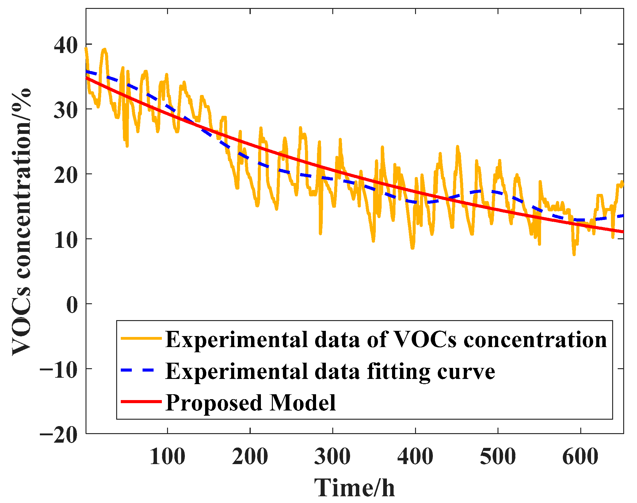
The SVE equipment was installed at the contaminated site for a period of time, with the set pressure maintained at 10 kPa and the air valve kept at a fixed opening. The experimental equipment was operated for 652 h from 11 March 2022 to 8 April 2022, and the extraction concentrations measured by the VOCs sensors in the pipeline at the extraction well outlet were measured during the operation period. As shown in Figure 8, the VOC concentration in the soil exhibited a decreasing trend from the initial 30–40% and eventually reached the 10–20% interval. Through field experiments, the variation of extraction concentration with time of operation of the equipment could be used to verify the effectiveness of the equipment in removing VOCs and remediating the soil, as well as the completion date. At the same time, the extraction concentrations calculated using the proposed model matched with the experimental data of the site, proving the validity of the model.
5. Conclusions
In this paper, a mathematical model was established for SVE equipment. The main influencing factors of the extraction process were analyzed through joint simulations of COMSOL and Simulink. It was shown that the fan speed was the main influencing factor for pressure and flow rate, demonstrating a linearly relationship; the opening of the fresh air valve led to a simultaneous and linear decrease in the extraction flow rate and in the well. An optimal operation strategy for intermittent extraction was developed using the proposed model to improve energy utilization efficiency by 23%. The ability of the SVE equipment to remove soil VOCs contaminants was demonstrated through simulations and field experiments, verifying the validity of the proposed model. Future work will be conducted on the SVE optimized operation strategy.
Author Contributions
Y.S. designed the study; S.Z. was a major contributor to writing the manuscriptl; Z.D. contributed to the creation of the experimental platform used in the work; Y.W. was in charge of the whole trial and substantively revised it; Y.Y. and Q.W. assisted with sampling, laboratory analyses, and equipment operation. All authors have read and agreed to the published version of the manuscript.
Funding
The research work presented in this paper was supported by the Youth Fund of the National Natural Science Foundation of China (grant numbers 52105044 and 52105046) and the Center International Group Company Limited.
Data Availability Statement
The data are not publicly available due to privacy. The data presented in this study are available on request from the corresponding author.
Conflicts of Interest
The authors declare no conflict of interest.
References
- Ye, S.; Zeng, G.; Wu, H.; Zhang, C.; Liang, J.; Dai, J.; Liu, Z.; Xiong, W.; Wan, J.; Wan, J.; et al. Co-occurrence and interactions of pollutants, and their impacts on soil remediation—A review. Crit. Rev. Environ. Sci. Technol. 2017, 47, 1528–1553. [Google Scholar] [CrossRef]
- Ossai, I.C.; Ahmed, A.; Hassan, A.; Hamid, F.S. Remediation of soil and water contaminated with petroleum hydrocarbon: A review. Environ. Technol. Innov. 2020, 17, 100526. [Google Scholar] [CrossRef]
- Wei, K.H.; Ma, J.; Xi, B.D.; Yu, M.D.; Cui, J.; Chen, B.L.; Li, Y.; Gu, Q.-B.; He, X.-S. Recent progress on in-situ chemical oxidation for the remediation of petroleum contaminated soil and groundwater. J. Hazard. Mater. 2022, 432, 128738. [Google Scholar] [CrossRef] [PubMed]
- Cao, W.; Zhang, L.; Miao, Y.; Qiu, L. Research progress in the enhancement technology of soil vapor extraction of volatile petroleum hydrocarbon pollutants. Environ. Sci. Process. Impacts 2021, 23, 1650–1662. [Google Scholar] [CrossRef] [PubMed]
- Qin, C.Y.; Zhao, Y.S.; Zheng, W.; Li, Y.S. Study on influencing factors on removal of chlorobenzene from unsaturated zone by soil vapor extraction. J. Hazard. Mater. 2010, 176, 294–299. [Google Scholar] [CrossRef]
- Brusseau, M.L.; Rohay, V.; Truex, M.J. Analysis of soil vapor extraction data to evaluate mass-transfer constraints and estimate source-zone mass flux. Groundw. Monit. Remediat. 2010, 30, 57–64. [Google Scholar] [CrossRef] [PubMed] [Green Version]
- Farhan, S.; Holsen, T.M.; Budiman, J. Interaction of soil air permeability and soil vapor extraction. J. Environ. Eng. 2001, 127, 32–37. [Google Scholar] [CrossRef]
- Yu, Y.; Liu, L.; Yang, C.; Kang, W.; Yan, Z.; Zhu, Y.; Wang, J.; Zhang, H. Removal kinetics of petroleum hydrocarbons from low-permeable soil by sand mixing and thermal enhancement of soil vapor extraction. Chemosphere 2019, 236, 124319. [Google Scholar] [CrossRef]
- Yasumoto, K.; Kawabata, J. Evaluation of in-situ air permeability test for designing of soil vapor extraction. In Groundwater Updates; Springer: Tokyo, Japan, 2000; pp. 393–397. [Google Scholar]
- Høier, C.K.; Sonnenborg, T.O.; Jensen, K.H.; Kortegaard, C.; Nasser, M.M. Experimental investigation of pneumatic soil vapor extraction. J. Contam. Hydrol. 2007, 89, 29–47. [Google Scholar] [CrossRef] [PubMed]
- Albergaria JT, Maria da Conceição M, and Delerue-Matos C, Soil vapor extraction in sandy soils: Influence of airflow rate. Chemosphere 2008, 73, 1557–1561. [CrossRef]
- Sun, M.; Ouyang, X.; Mattila, J.; Yang, H.; Hou, G. One Novel Hydraulic Actuating System for the Lower-Body Exoskeleton. Chin. J. Mech. Eng. 2021, 34, 31. [Google Scholar] [CrossRef]
- Labianca, C.; De Gisi, S.; Picardi, F.; Todaro, F.; Notarnicola, M. Remediation of a petroleum hydrocarbon-contaminated site by soil vapor extraction: A full-scale case study. Appl. Sci. 2020, 10, 4261. [Google Scholar] [CrossRef]
- Yoon, H.; Oostrom, M.; Wietsma, T.W.; Werth, C.J.; Valocchi, A.J. Numerical and experimental investigation of DNAPL removal mechanisms in a layered porous medium by means of soil vapor extraction. J. Contam. Hydrol. 2009, 109, 1–13. [Google Scholar] [CrossRef] [PubMed]
- Ouoba, S.; Bénet, J.C. Numerical modeling and simulation of water transfer in soil with low water contents. Int. J. Environ. Sci. Technol. 2022, 1–12. [Google Scholar] [CrossRef]
- Ding, Y.; Zhang, Y.; Deng, Z.; Song, H.; Wang, J.; Guo, H. An innovative method for soil vapor extraction to improve extraction and tail gas treatment efficiency. Sci. Rep. 2022, 12, 6495. [Google Scholar] [CrossRef]
- Fen, C.S.; Chan, C.; Cheng, H.C. Assessing a response surface-based optimization approach for soil vapor extraction system design. J. Water Resour. Plan. Manag. 2009, 135, 198. [Google Scholar] [CrossRef]
- Kacem, M. Models for soil vapor extraction and multiphase extraction design and monitoring. In Diagnostic Techniques in Industrial Engineering; Springer: Cham, Switzerland, 2018; pp. 171–190. [Google Scholar]
- Zhao, L.; Zytner, R.G. Three-dimensional numerical model for soil vapor extraction. J. Contam. Hydrol. 2013, 147, 82–95. [Google Scholar]
- Carroll, K.C.; Oostrom, M.; Truex, M.J.; Rohay, V.J.; Brusseau, M.L. Assessing performance and closure for soil vapor extraction: Integrating vapor discharge and impact to groundwater quality. J. Contam. Hydrol. 2012, 128, 71–82. [Google Scholar] [CrossRef]
- Shi, H.; Li, J.; Guo, L.; Mei, X. Control Performance Evaluation of Serial Urology Manipulator by Virtual Prototyping. Chin. J. Mech. Eng. 2021, 34, 25. [Google Scholar] [CrossRef]
- Esslimani, K.; Kacem, M.; Boudouch, O.; Elkacmi, R.; Benadda, B. Influence of the presence of clay and water on the efficiency of soil vapor extraction in sand laboratory columns. Remediat. J. 2022, 33, 63–76. [Google Scholar] [CrossRef]
- Johnson, C.D.; Byrnes, M.E. Hanford 200-PW-1 Operable Unit Soil Vapor Extraction Endpoint Evaluation. Remplex Semin. Present. Jan. 2021, 26, 2021. [Google Scholar]
- Zhang, Y.; Li, K.; Xu, M.; Liu, J.; Yue, H. Medical Grabbing Servo System with Friction Compensation Based on the Differential Evolution Algorithm. Chin. J. Mech. Eng. 2021, 34, 107. [Google Scholar] [CrossRef]
- Wang, N.; Liu, Q.; Shi, Y.; Wang, S.; Zhang, X.; Han, C.; Wang, Y.; Cai, M. Modeling and Simulation of an Invasive Mild Hypothermic Blood Cooling System. Chin. J. Mech. Eng. 2021, 34, 23. [Google Scholar] [CrossRef]
- Shi, Y.; Rui, S.; Xu, S.; Wang, N.; Wang, Y. COMSOL Modeling of Heat Transfer in SVE Process. Environments 2022, 9, 58. [Google Scholar] [CrossRef]
- Jin, Z. Numerical Simulation Study on Multi-well Overlapping Effect of Soil Vapor Extraction. Master’s Thesis, Guangdong University of Technology, Guangzhou, China, 2017. [Google Scholar]
- Barnes, D.L. Estimation of operation time for soil vapor extraction systems. J. Environ. Eng. 2003, 129, 873–878. [Google Scholar] [CrossRef]
- Modeling the Rebounding of Contaminant Concentrations in Subsurface Gaseous Phase during Intermittent Soil Vapor Extraction Operation. J. Chin. Inst. Environ. Eng. 2007, 17, 11–19.
Figure 1.
Flow direction of normal-temperature SVE process.

Figure 2.
Pressure in soil distribution: (a) longitudinal section; (b) cross-section.
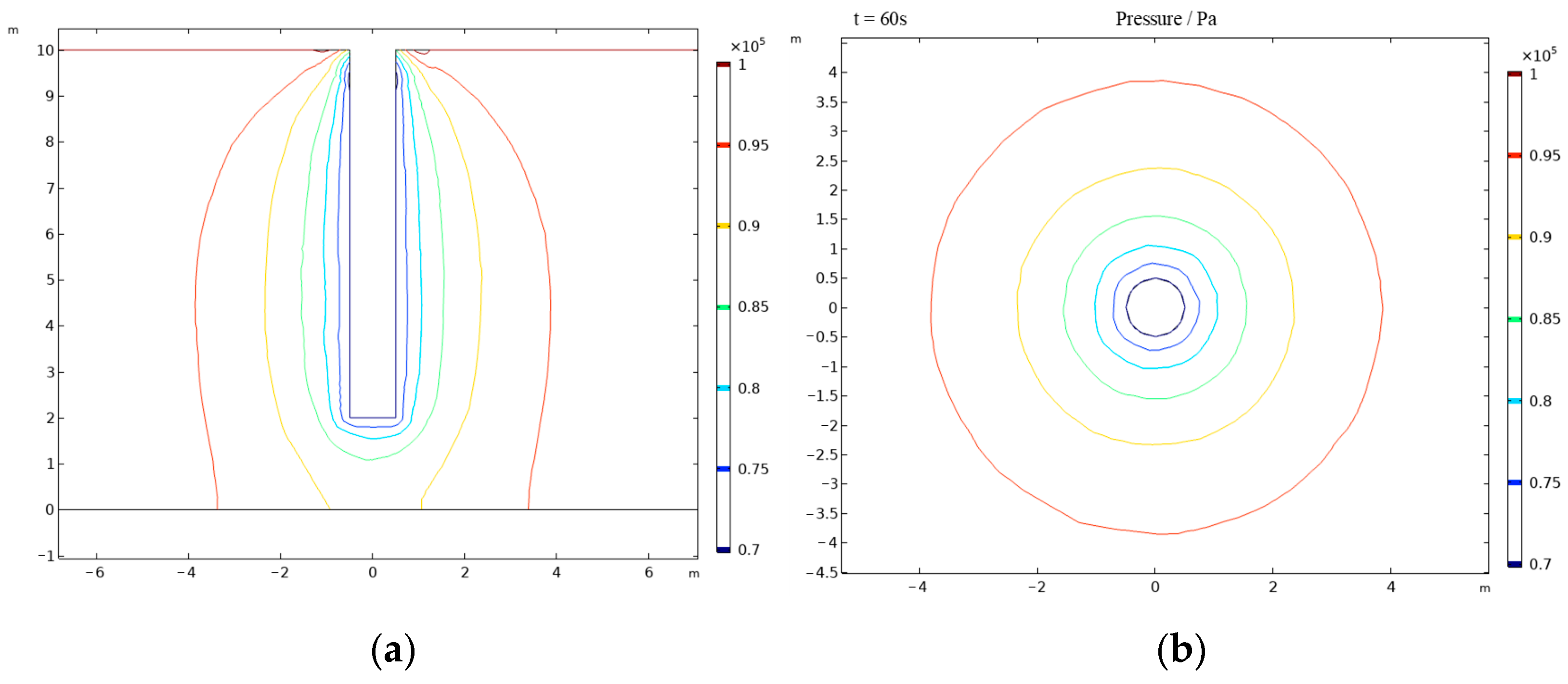
Figure 3.
The response curve of (a) extraction flow and (b) pressure.
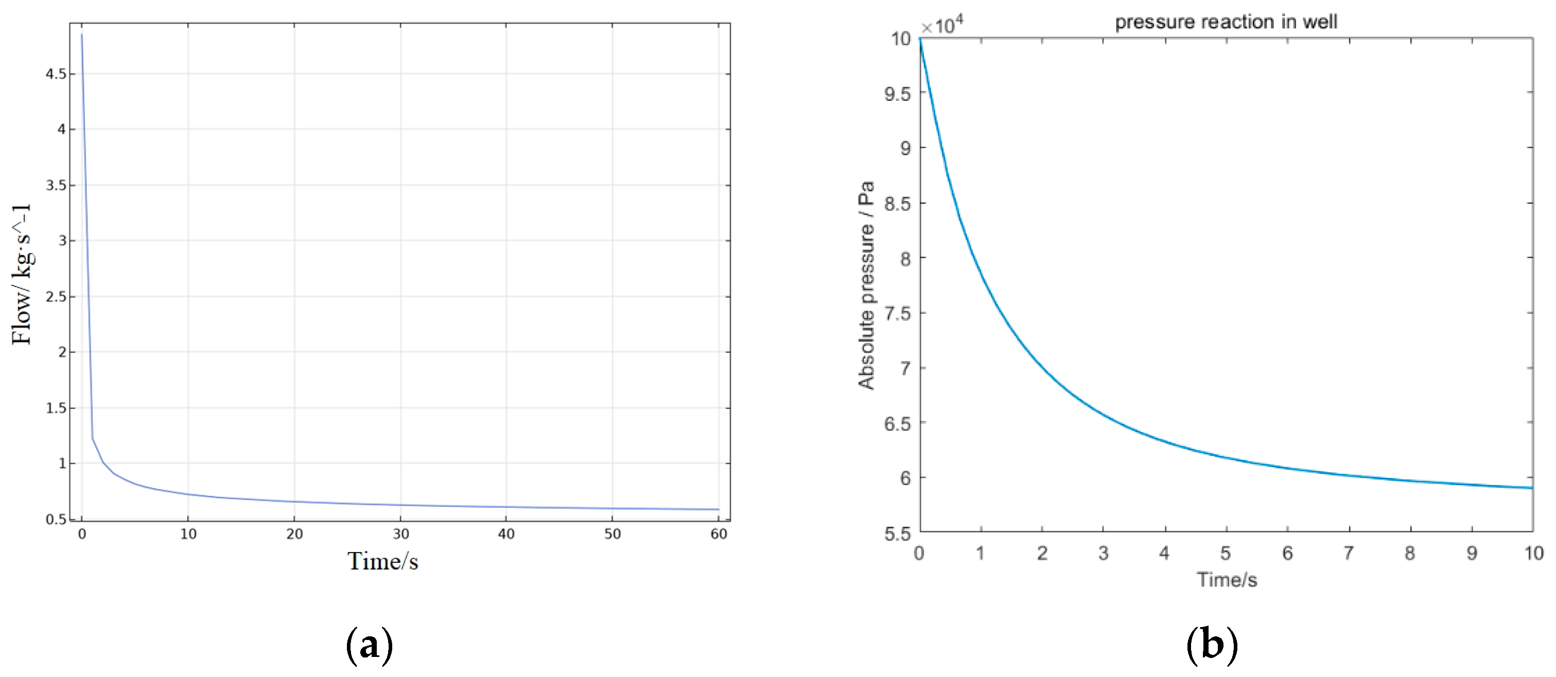
Figure 4.
Relationship between the pressure in the well and frequency of the fan.

Figure 5.
The response curve of flow with (a) the fresh air valve opened and closed; (b) the relationship of flow and pressure in different opening.
Figure 5.
The response curve of flow with (a) the fresh air valve opened and closed; (b) the relationship of flow and pressure in different opening.

Figure 6.
The dynamic curve of (a) pressure in well; (b) flow of the extraction.
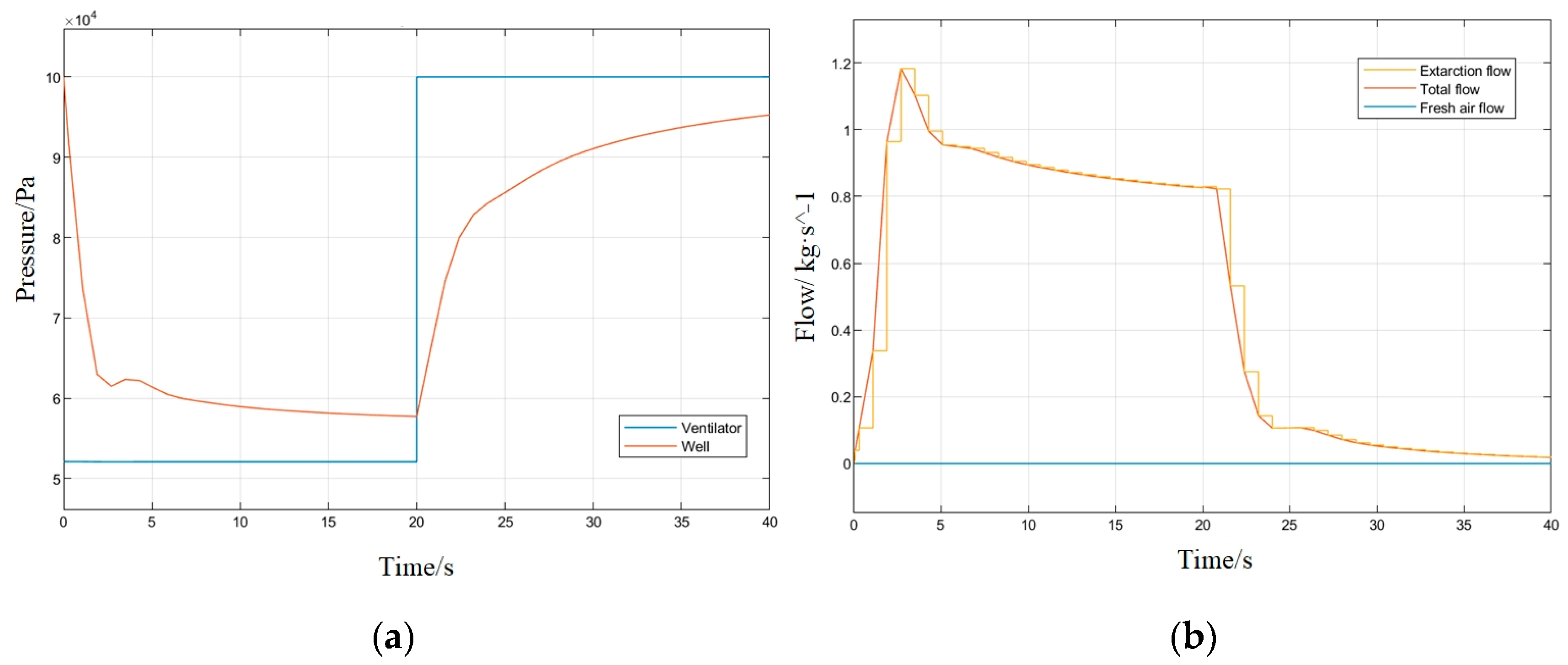
Figure 7.
The influence of closing the fresh air valve on the flow of extraction and pressure at the inlet of a ventilator at different frequencies.
Figure 7.
The influence of closing the fresh air valve on the flow of extraction and pressure at the inlet of a ventilator at different frequencies.
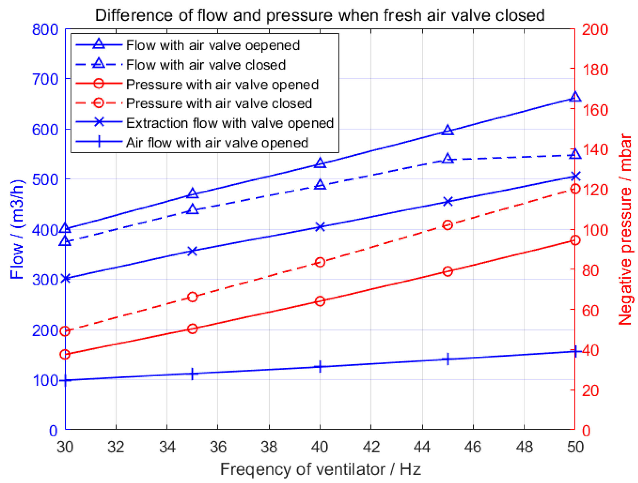
Figure 8.
VOC concentration in the extraction pipeline in the field experiments.
Disclaimer/Publisher’s Note: The statements, opinions and data contained in all publications are solely those of the individual author(s) and contributor(s) and not of MDPI and/or the editor(s). MDPI and/or the editor(s) disclaim responsibility for any injury to people or property resulting from any ideas, methods, instructions or products referred to in the content. |
© 2022 by the authors. Licensee MDPI, Basel, Switzerland. This article is an open access article distributed under the terms and conditions of the Creative Commons Attribution (CC BY) license (https://creativecommons.org/licenses/by/4.0/).
Share and Cite
MDPI and ACS Style
Shi, Y.; Zhao, S.; Diao, Z.; Ye, Y.; Wang, Q.; Wang, Y. Modeling and Analysis of the Soil Vapor Extraction Equipment for Soil Remediation. Electronics 2023, 12, 151. https://doi.org/10.3390/electronics12010151
AMA Style
Shi Y, Zhao S, Diao Z, Ye Y, Wang Q, Wang Y. Modeling and Analysis of the Soil Vapor Extraction Equipment for Soil Remediation. Electronics. 2023; 12(1):151. https://doi.org/10.3390/electronics12010151
Chicago/Turabian StyleShi, Yan, Shijian Zhao, Zhuo Diao, Yuan Ye, Qiansuo Wang, and Yixuan Wang. 2023. "Modeling and Analysis of the Soil Vapor Extraction Equipment for Soil Remediation" Electronics 12, no. 1: 151. https://doi.org/10.3390/electronics12010151
Note that from the first issue of 2016, this journal uses article numbers instead of page numbers. See further details here.