Coordination Control of a Hybrid AC/DC Smart Microgrid with Online Fault Detection, Diagnostics, and Localization Using Artificial Neural Networks

Abstract

In this paper, a solar and wind renewable energies-based hybrid AC/DC microgrid (MG) is proposed for minimizing the number of DC/AC/DC power conversion processes. High penetration rates of renewable energy increase MG instability. This instability can be mitigated by maintaining a balance between consumption demand and production levels. Coordination control is proposed in this study to address coordinated electricity flowing through both AC and DC links and to achieve system stability under variability of generation, load, and fault conditions. The MG adopts a bidirectional main converter that is controlled using a digital proportional resonant (PR) current controller in a synchronous reference frame. The PR controller plays a role as a digital filter with infinite impulse response (IIR) characteristics by virtue of its high gain at the resonant frequency, thereby reducing harmonics. Moreover, the applied PR controller quickly follows the reference signal, can adapt to changes in grid frequency, is easy to set up, and has no steady-state error. Moreover, the solar photovoltaic (PV)-based distribution generation (DG) is supported by a maximum power point tracker (MPPT)-setup boost converter to extract maximum power. Due to the usage of converter-connected DG units in MGs, power electronic converters may experience excessive current during short circuit faults. Fault detection is critical for MG control and operation since it empowers the system to quickly isolate and recover from faults. This paper proposed an intelligent online fault detection, diagnostic, and localization information system for hybrid low voltage AC/DC MGs using an artificial neural network (ANN) due to its accuracy, robustness, and quickness. The proposed scheme enables rapid detection of faults on the AC bus, resulting in a more reliable MG. To ensure the neural network’s validity, it was trained on various short circuit faults. The performance of the MG was evaluated using MATLAB software. The simulation findings indicate that the suggested control strategy maintains the dynamic stability of the MG, meets the load demand, and achieves energy balance as well as properly predicts faults.

1. Introduction

Environmental pollution and a slew of other issues have gained prominence in recent years as a result of widespread reliance on fossil fuels that may run out by the end of the century. To address this dilemma, environmentally friendly renewable energy is harnessed and converted into electrical energy, which not only diversifies energy consumption but also reduces reliance on fossil fuels for power generation. This energy is generated through a variety of long-term sources, including solar, wind, and other renewable sources, all of which are increasingly being used to power MGs. Among other characteristics, a conventional power system is one in which individual grids are interconnected to form a larger, centralized network. In comparison to a traditional power system, an MG system is more compact, independent, and decentralized. Distribution energy resources (DERs) are utilized to connect various types of power technologies to loads by transmitting electricity through transmission/distribution subsystems in a short amount of time. MGs respond to specific consumer demands; increase local reliability; preserve local frequency and voltage; and so on [1,2,3]. The term “DERs” refers to smaller, geographically scattered generating resources, such as solar and wind, that are connected to the local distribution grid. Depending on their capacity and arrangement, DERs can either fully or partially meet consumer demand for electricity or replenish the distribution system with any extra energy. Certain DERs, such as electric storage systems, are entirely controlled, which enables the resolution of operational restrictions on transmission and distribution networks [4]. If the DERs are linked to the grid, they may be divided into two categories: nondispatchable ones, such as solar units or wind turbines, and dispatchable ones, such as fuel cells and microturbines as well as energy storage units. While nondispatchable DERs must generate electricity at full capacity, dispatchable DERs must be regulated in cooperation to meet the intended power demand planned by a high-level strategy aimed at lowering the cost while maintaining full capacity [5,6,7]. Moreover, a hybrid system that contains solar and energy storage system (ESS) units may have the least energy exchange with the grid due to the size of the PV system and ESS. One of the main issues with such systems is the need to separate the PV system and loads from the utility grid. This will disrupt the system’s energy supply [8]. Bilateral hybrid inverters are used in hybrid systems. When the distribution network is unplugged, the inverters should disconnect from the grid and reconnect to the PV systems and loads [9,10]. Numerous control techniques, such as dead-beat (DB) controllers, hysteresis, proportional integral (PI) controllers, and PR controllers, can be used to integrate power systems and inverter-based DGs. While hysteresis control is simple and responsive, the output current has large ripples, resulting in poor current quality and complicating output filter design [11]. The use of DB predictive control is common because it works well with current-controlled DGs. It is, however, extremely complex and highly reliant on system settings [12]. The digital PR control technique in a synchronous reference frame is popular for reducing steady-state error, correcting many harmonics behind sinusoidal signals and regulating them whereas PI controllers provide more steady-state error and are coherent with the parameter setting problem [4]. It is essential to use optimization algorithms and artificial intelligence to select PI controller parameters optimally, but this will increase the control method’s complexity. Consequently, it is essential to compute the control parameters in a system with minimal complexity. Using a PR controller, grid frequency and resonant filter frequency must be equal for optimal performance [13]. The reference [14] proposes modeling a PR controller for a grid-connected inverter and observing its performance under load fluctuation conditions. There are a number of references in the literature for grid-connected inverters (GCIs) that use PR controllers. There have been only a few studies that describe the approach to design a PR controller [15,16].

Other challenges include issues related to the faults in MGs that can arise as a result of a variety of factors, including feeder line short circuits, joint failures of overhead lines and cables, the failure of one or more phases of a circuit breaker, and the melting of fuses or conductors, among others. Traditional fault detection schemes become ineffective in MGs as a result of the widespread use of inverter-interfaced distributed generation, which is affected by large fault currents. Intelligent fault detection schemes are intended to quickly pinpoint the location and type of faults so MGs can be protected and services can be restored. They are also intended to provide fast fault location [17]. In this context, the researchers in [18] presented a fault detection approach for MGs. A new fault detection method and fault criteria are proposed based on the phase differences between bus voltages’ positive-sequence fault components and current feeders’ positive-sequence fault components. The reference [19] provided a method for detecting faults based on the phase change of negative-sequence currents. In [20], a voltage-independent way to find faults was presented. It examines the current fault component phase data from a minimum of three feeders that connect to the bus bar to figure out which way the fault is coming from. In most cases, fault location in AC grids can be accomplished using a traveling-wave algorithm or another algorithm based on injection [21,22]. However, the algorithms of traveling waves have issues with detecting and discriminating reflected waves, and some of them require data to be synchronized across communication connections. None of them evidenced fault localization capability on islanded MGs or networks with loop/ring topologies. Meanwhile, algorithms based on injection are only applicable to phase-to-ground faults and are limited to radial networks [23,24]. Numerous fault diagnosis models are being considered for the classification of MG faults [25,26,27,28]. The reference [29] described a method for declaring a fault type by transforming the output of distributed generators (DGs) from abc to dq. There are many other techniques used in fault investigation, such as frequency and/or time-based methods, including the time-domain reflectometer (TDR), frequency-domain reflectometer (FDR), and frequency- and time-based methods, such as the time–frequency domain reflectometer (TFDRs) method. A TDR has the following drawbacks [30]: (i) It cannot pinpoint the exact location and only provides an approximation of the fault location distance. (ii) High-resistance ground faults are typically not detectable using a TDR. (iii) The TDR signal is distorted by the ambient electrical noise. The FDR method and other frequency-based methods are more precise than the TDR method due to the use of power signals as incident signals and the application of the Fourier transform to locate wire faults. The TDR method requires more calculations and processing time, so identifying wire faults is difficult [31]. The complexity of frequency-based methods means they are rarely used effectively today. In addition to being more precise and requiring less processing time for the classification and localization of faulty signals, the advancement of machine learning techniques is attracting more interest in fault analysis [32]. Some algorithms [33,34,35,36] can be used for extracting signal features for fault detection and classification in distributions lines and MGs, including the mentioned frequency-based methods, the fast Fourier transform (FFT), discrete Fourier transform (DWT), and other statistical techniques, which are then applied to an ML algorithm. All of the methods mentioned in [30,31,32,33,34,35,36] required significantly more computations and processing time. Because of this, a fast processor with a high sampling frequency is required for implementation. Due to the high upfront cost of implementing phasor measurement units (PMUs), determining the optimum number of PMUs to be deployed is regarded as a crucial necessity in the design of contemporary power systems, which in turn increases the method’s complexity [37]. The machine learning in references [38,39,40] and the shallow architecture used by neural network-based methods hinder an MG’s ability to learn from its complex nonlinear features. Due to the absence of hidden layers, these strategies are unable to combine the advantages of multiple features with perfection.

The research literature contains a significant number of references to GCI in combination with PR controllers. Few studies describe PR controller design in the digital domain. Most research illustrates PR controller applications without a systematic method for establishing control parameters while other research focuses on continuous-time modeling. The reader must digitally use the PR controller with a systematic design method. In this work, the main converter of a hybrid DC/AC MG has been controlled with a PR current controller in a coordinated manner in order to minimize multiple uses of power electronic conversions. Moreover, another research gap in the progression of MG fault detection systems persists. Certain existing studies lack information about the type of fault and thus cannot be properly applied to the single-phase tripping paradigm (see [41,42]). Additionally, the majority of research focuses exclusively on the fault issues in DC MGs. Moreover, other research focuses on offline fault detection. Moreover, there is a dearth of research devoted to simultaneously detecting, diagnosing, and locating faults. The following summarizes the main contributions of this work:

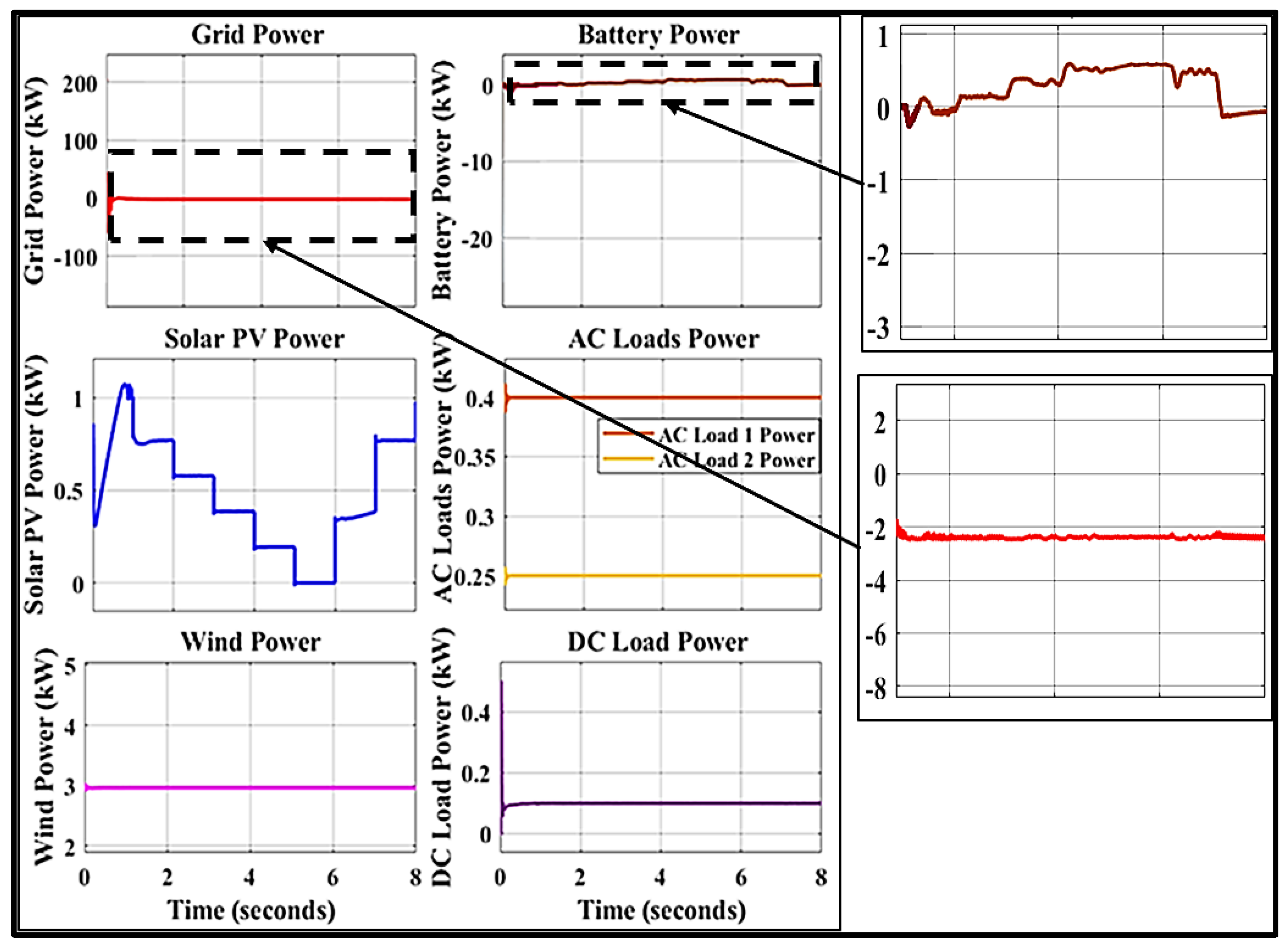
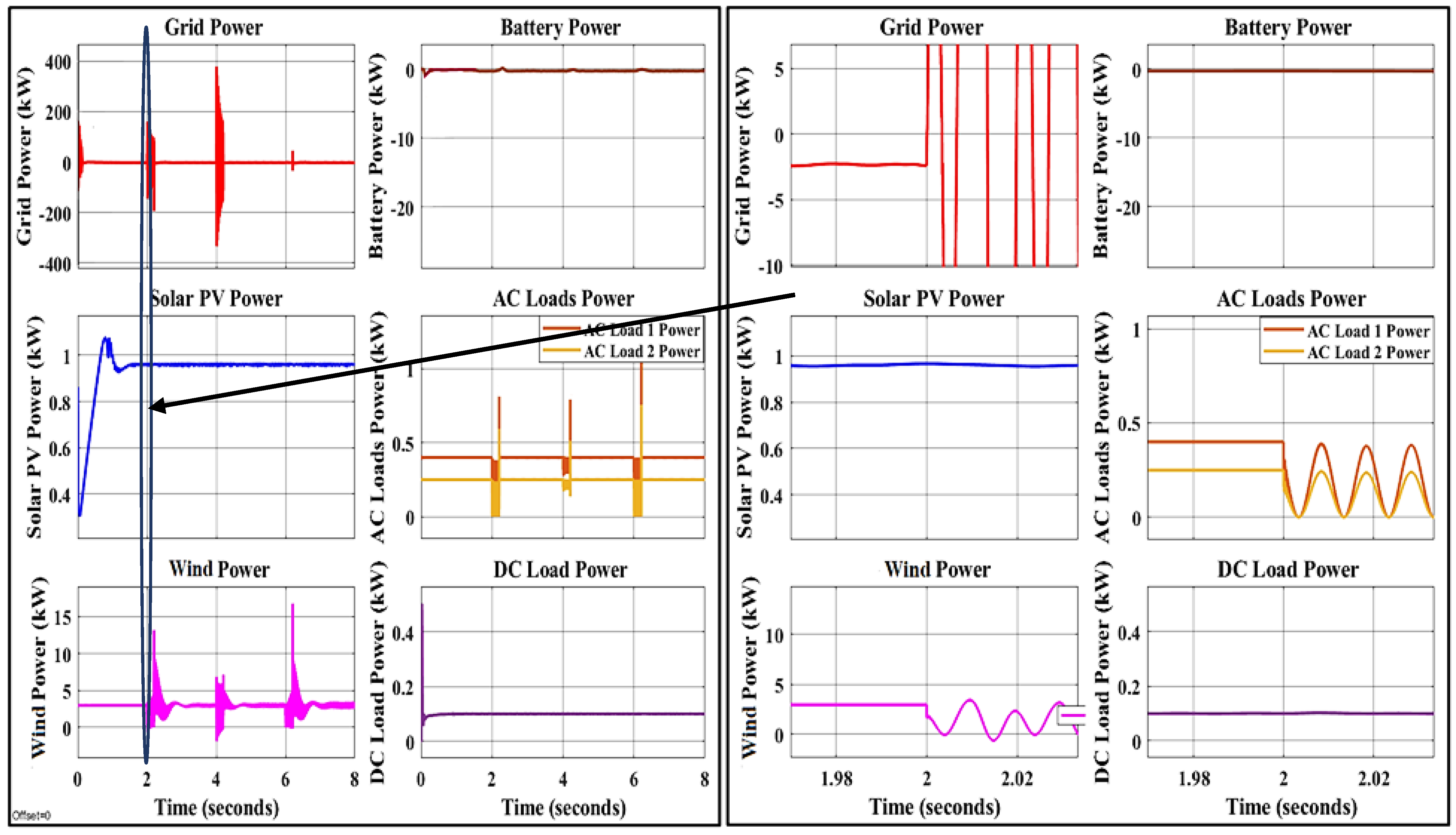
• As a means of reducing DC/AC/DC power electronic conversions, this paper proposes a hybrid AC/DC grid-connected MG with renewable and storage energies. The proposed work addresses the coordination of power flow between the AC bus and DC bus in order to maintain an energy balance between demand and supply and to achieve system stability under a variety of load and generation conditions.
• This paper discusses the design process for an inverter-integrated digital current PR controller in a synchronous reference frame. The resonant and proportional gains as well as resonance path coefficients are all calculated step by step. One of its most important contributions is to make the work of researchers to create digitally controlled inverters easier. This paper will also include a digital PR controller’s frequency-domain analysis. This study used a fictitious w-domain. Digital PR power and current controllers designed using the proposed procedure were used in the case study to demonstrate the inverter’s efficacy.
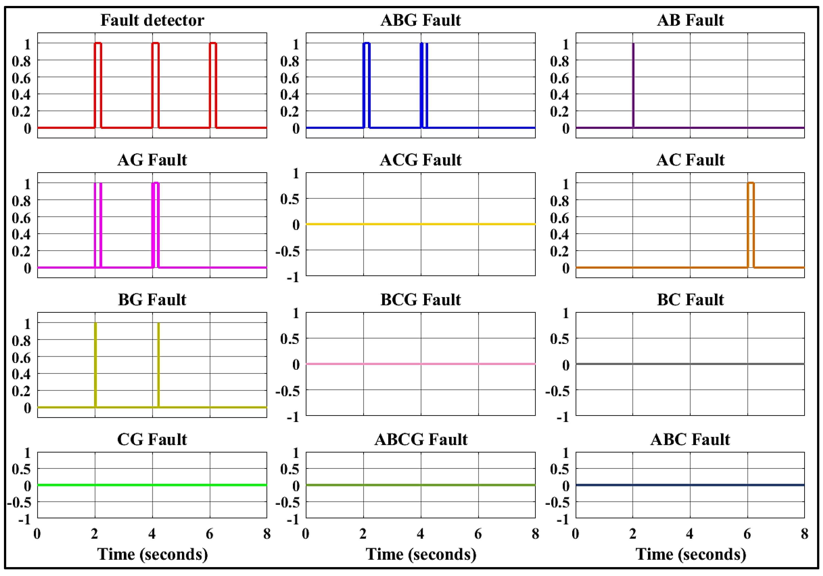
• This paper proposed three ANN-based intelligent fault detection, diagnostic, and location schemes for the adopted AC/DC MGs. The proposed system allows for the rapid online detection, classification, and localization of faults on the AC bus, resulting in a more reliable MG. A proposed fault detection mechanism is capable of providing precise and timely details about the type, phase, and location of faults.

The following is the format for the remainder of this paper: System configuration, operations, and modeling are described in Section 2. System resources modeling is discussed in Section 3. Coordination converter control is presented in Section 4. Section 5 details the ANN methodology. The ANN-based fault detection, diagnosis, and localization are presented in Section 6. The proposed ANN process is discussed in Section 7. We evaluate the performance of the proposed controller through extensive simulation studies in Section 8. This paper’s conclusion can be found in Section 9.

2. System Configuration, Operation, and Modeling

2.1. System Configuration

The proposed AC/DC MG structure is depicted in Figure 1, which consists primarily of wind energy, solar photovoltaic generation, storage systems, AC loads, DC load, and an AC main grid connection. To simulate system operation and control, the proposed MG was modeled using Simulink in a MATLAB environment. To simulate DC sources, the 1 kW PV panel was linked to the DC bus via a boost converter. A capacitor C_PV was adopted to reduce the PV voltage’s high-frequency ripples. A 3 kW wind turbine with a doubly fed induction generator (DFIG) was hooked up to an AC bus to make it look like an AC source. To store energy, a bidirectional buck-boost converter linked a 400 Ah battery to the DC bus. The (0.1 kW) DC load and (0.25 kW and 0.40 kW) AC loads were connected to the DC bus and AC bus, respectively. For DC and AC buses, the rated voltages were 470 V and 400 V, respectively. Through an isolation transformer, the DC bus and AC bus were linked by a three-phase bidirectional DC/AC main converter equipped with an RLC power filter. The additional parameters of the MG are shown in

Table 1. The MG parameters.

Parameter Name	Acronym	Value
Input booster capacitor	$C_{PV}$	0.00875 f
Output booster capacitor	$C_d$	500 μf
Boost inductance	$L_1$	0.0105 H
Inverter filter resistor	$R_f$	0.05 Ω
Inverter filter inductance	$L_f$	10 mH
Inverter filter inductance	$C_f$	100 μF
AC side voltage	$V_{AC}$	400 V
DC side voltage	$V_{DC}$	470 V
Input buck-boost capacitor	$C_{in}$	500 μF
Output buck-boost capacitor	$C_{out}$	500 μF
Buck-boost inductance	$L$	0.0105 H
Battery nominal voltage	$V_{Bat}$	400 V
Initial state of charge	SOC	71%
3Ph PI section line length	$D$	10 km
Main grid voltage	$V$	34.5 kV
Main grid power	$P$	154 MW
System frequency	$F$	50 Hz

.

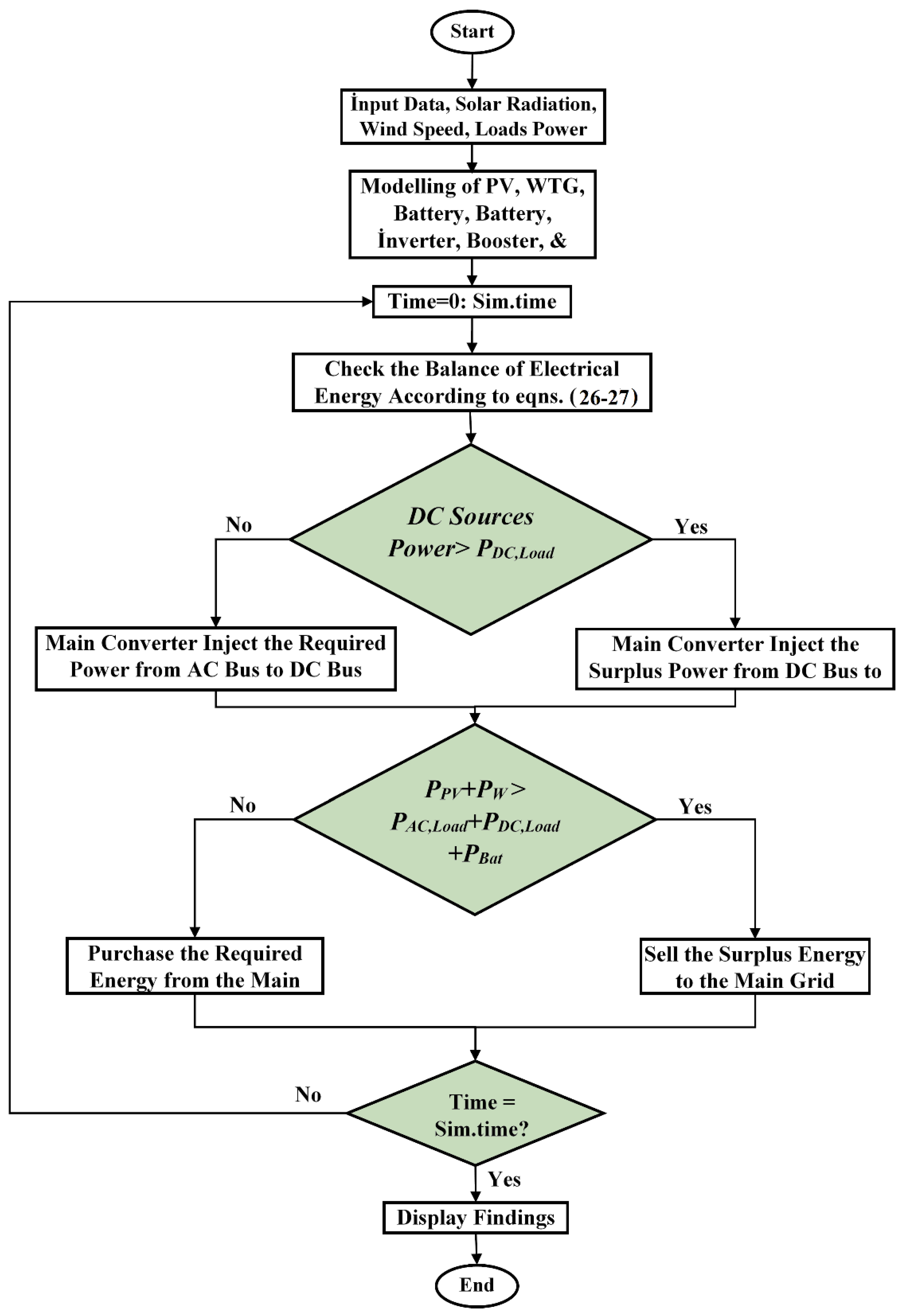
2.2. System Operation

The MG is capable of operating in two modes of operation. The primary converter’s function in grid-tied mode is to maintain stable voltage on the DC bus and to swap power between the AC bus and DC bus. The boost converter is controlled to deliver the maximum amount of power possible from solar PV. When the output power of the DC sources exceeds the input power of the DC loads, the power converter represents an inverter, injecting power from the DC bus to the AC side and vice versa. When the total power generation in the hybrid grid exceeds the total load, the utility grid obtains more power. Otherwise, the hybrid grid will be supplied with electricity by the utility grid. Figure 2 illustrates the system’s operating strategy.

When operating in grid-tied mode, the battery converter is not as crucial because the power grid handles load balancing. The battery is critical in autonomous mode for power balance and voltage stability. The energy management system (EMS) regulates various converters by assigning control objectives. Boost and battery converters are used in stabilizing the DC bus voltage under various operating conditions. The main converter is controlled by two digital PR current controllers in a synchronous reference frame to ensure the stability and quality of the AC bus voltage. Solar PV systems can operate in MPPT or off-MPPT modes depending on the system’s operational requirements. The wind turbine and PV panel are subjected to wind speeds and solar irradiance, respectively, to predict the power variation of AC and DC resources and to validate the MPPT control algorithm.

3. System-Generation Resources Modeling

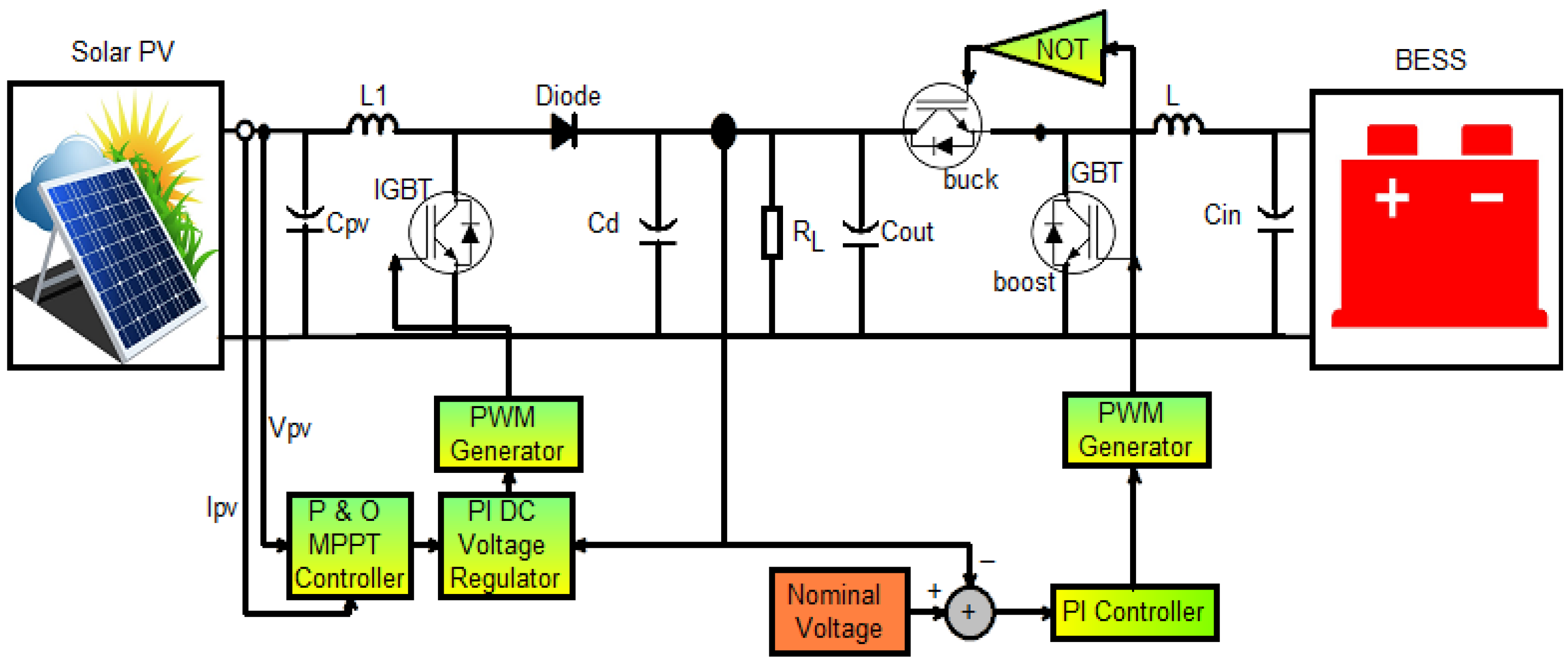
3.1. Solar Photovoltaic

The equation that defines the I-V behavior of the PV cell circuit model with one diode and two resistors is given in Equation (1) [43].

$$I=I_{PV}-I_O\left\{\mathit{exp}\left(\frac{V+I{R}_s}{\alpha V_T}\right)-1\right\}-\frac{V+I{R}_s}{R_{sh}}$$

(1)

where $I_{PV}$ represents the photocurrent, $R_s$ means the series resistor, $I_O$ is the diode reverse saturation current, α is the ideality factor that explains how far the diodes deviate from their ideal state,$R_{sh}$ is the shunt resistor that accounts for current leakage through highly conductive shunts across the p–n junction, and $V_T$ is the thermal voltage of the diode and is influenced by the electron charge ($q$), the number of series connected cells ($n$), the Boltzmann constant ($k$), and the temperature ($T$) of the diode.

$$V_T=n\frac{kT}{q}$$

(2)

The amount of solar irradiation that hits the module and the temperature of the PV cells together determines the photocurrent ($I_{PV}$), as shown in the following equation.

$$I_{PV}=\frac{(I_{PHO,n}+k_i\Delta T)G}{G_{ref}}$$

(3)

where $\Delta T$ is the deviation in temperature between the PV cell’s reference temperature and the actual one, $G_{ref}$ acts the nominal irradiance, and $I_{PHO,n}$ means the photocurrent predicted at the nominal condition (typically 25 °C and 1000 Watt/m² irradiance). Solar irradiance ($G$) and temperature coefficient ($k_i$) are both expressed in watts per square meter.

Equation (4) shows how temperature affects the open circuit voltage $V_{o.c}$:

$$V_{o.c}=V_{oc,n}+k_v\Delta T$$

(4)

where $k_v$ represents the open-circuit voltage temperature coefficient, and $V_{oc,n}$ is the $V_{o.c}$ at normal temperature. By solving for it, the saturation current of this diode, $I_o$, can be determined.

$$I_o=\frac{I_{S,N}+k_i\Delta T}{e^{\left(\frac{V_{oc,n}+k_v\Delta T}{\alpha V_T}\right)}-1}$$

(5)

where $I_{S,N}$ stands for the short circuit current under standard circumstances.

3.2. Wind Turbine Generator (WTG)

A WTG’s power output is determined by Equation (6) [44].

$$P_W=0.5A\rho C_p\left(\gamma ,\beta \right)V_w^3$$

(6)

where $\rho$ denotes the air density, $A$ denotes the rotor swept area, $V_w$ denotes the wind speed, and $C_p$ denotes the power coefficient, which is a function of the pitch angle $\beta$ and tip speed ratio $\gamma$.

A DFIG’s mathematical models are critical components of its control system. Here are the equations for the voltage produced by a rotating $dq$-coordinate system in an induction motor [44]:

$$\left[\begin{array}{c}{v}_{ds}\\ v_{qs}\\ \begin{array}{c}{v}_{dr}\\ v_{qr}\end{array}\end{array}\right]=\left[\begin{array}{c}\begin{array}{ccc}-R_s& 0& \begin{array}{cc}0& 0\end{array}\end{array}\\ \begin{array}{ccc}0& -R_s& \begin{array}{cc}0& 0\end{array}\end{array}\\ \begin{array}{c}\begin{array}{ccc}0& 0& \begin{array}{cc}{R}_r& 0\end{array}\end{array}\\ \begin{array}{ccc}0& 0& \begin{array}{cc}0& R_r\end{array}\end{array}\end{array}\end{array}\right]\left[\begin{array}{c}{i}_{ds}\\ i_{qs}\\ \begin{array}{c}{i}_{dr}\\ i_{qr}\end{array}\end{array}\right]+p\left[\begin{array}{c}{\lambda }_{ds}\\ {\lambda }_{qs}\\ \begin{array}{c}{\lambda }_{dr}\\ {\lambda }_{qr}\end{array}\end{array}\right]+\left[\begin{array}{c}-{\omega }_1{\lambda }_{ds}\\ {\omega }_1{\lambda }_{qs}\\ \begin{array}{c}-{\omega }_2{\lambda }_{dr}\\ {\omega }_2{\lambda }_{qr}\end{array}\end{array}\right]$$

(7)

$$\left[\begin{array}{c}{\lambda }_{ds}\\ {\lambda }_{qs}\\ \begin{array}{c}{\lambda }_{dr}\\ {\lambda }_{qr}\end{array}\end{array}\right]=\left[\begin{array}{c}\begin{array}{ccc}-L_s& 0& \begin{array}{cc}{L}_m& 0\end{array}\end{array}\\ \begin{array}{ccc}0& -L_s& \begin{array}{cc}0& L_m\end{array}\end{array}\\ \begin{array}{c}\begin{array}{ccc}-L_m& 0& \begin{array}{cc}{L}_r& 0\end{array}\end{array}\\ \begin{array}{ccc}0& -L_m& \begin{array}{cc}0& L_r\end{array}\end{array}\end{array}\end{array}\right]\left[\begin{array}{c}{i}_{ds}\\ i_{qs}\\ \begin{array}{c}{i}_{dr}\\ i_{qr}\end{array}\end{array}\right]$$

(8)

The DFIG’s dynamic equation:

$$\frac{J}{n_p}\frac{d{\omega }_r}{dt}=T_m-T_{em}=T_m-n_p{L}_m\left(i_{qs}{i}_{dr}-i_{qr}{i}_{ds}\right)$$

(9)

where the subscripts $d$, $q$, $s$, and $r$ denote the $d$-axis, $q$-axis, stator, and rotor, respectively; $L$ denotes the inductance; $\lambda$ denotes the flux linkage; $v$ stands for voltage; $i$ stands for current; ${\omega }_1$ and ${\omega }_2$ denote the angular synchronous and slip speeds, respectively, and ${\omega }_2$ = ${\omega }_1-{\omega }_r$; $T_m$ denotes the mechanical torque; $R_s$ and $L_s$ are the stator resistance and stator inductance, respectively; $L_r$ and $R_r$ are the rotor inductance and resistance, respectively; $n_p$ denotes the number of poles; $L_m$ denotes the mutual inductance; and $J$ is the rotor inertia constant.

Specifically, if the synchronously rotating $dq$-reference is directed by the stator voltage vector, then the $d$-axis will be aligned with the stator voltage vector and the $q$-axis will be aligned with the stator flux reference frame. As a result, ${\lambda }_{ds}=0$ and ${\lambda }_{qs}={\lambda }_s$. In the stator voltage-oriented reference frame, the following equations can be found [44]:

$$i_{ds}=-\frac{L_m}{L_s}{i}_{dr},T_{em}=n_p\frac{L_m}{L_s}{\lambda }_s{i}_{dr}$$

(10)

$$\sigma =\frac{L_s{L}_r-L_m{}^2}{L_s{L}_r}$$

(11)

$$v_{dr}=R_r{i}_{dr}+\sigma L_r\frac{d{i}_{dr}}{dt}-\left({\omega }_1-{\omega }_r\right)\left(L_m{i}_{qs}+L_r{i}_{qr}\right)$$

(12)

$$v_{qr}=R_r{i}_{qr}+\sigma L_r\frac{d{i}_{qr}}{dt}+\left({\omega }_1-{\omega }_r\right)\left(L_m{i}_{ds}+L_r{i}_{dr}\right)$$

(13)

3.3. Battery Energy Storage System (BESS)

Two critical features for representing the BESS state are the terminal voltage and SOC, which are shown as follows [45]:

$$V_o=V_b+R_b{i}_b-K\frac{Q}{Q+{\displaystyle \int }{i}_{b}dt}+A.e^{B{\displaystyle \int }{i}_{b}dt}$$

(14)

$$SOC=100\left(1+\frac{{\displaystyle \int }{i}_{b}dt}{Q}\right)$$

(15)

where $R_b$ is the battery’s internal resistance, $V_o$ is its open circuit voltage, $i_b$ represents charging current, $K$ acts as the polarization voltage, $Q$ is capacity, $A$ denotes exponential voltage, and $B$ represents total storage capacity.

3.4. Boost Converter

In the boost converter, the output voltage and current equations are described as follows:

$$V_{PV}+V_t=L_1\frac{d{i}_1}{dt}+R_1{i}_1$$

(16)

$$I_{PV}+i_1=C_{pv}.\frac{d{V}_{PV}}{dt}$$

(17)

$$V_T=V_d\left(1-D_1\right)$$

(18)

$$i_1\left(1-D_1\right)-C_d\frac{d{V}_{PV}}{dt}-\frac{V_d}{R_L}-i_b-i_{AC}$$

(19)

where $V_{PV}$ is the solar panel output voltage, $V_t$ is the terminal voltage across boost controllable switch, $L_1$ is the main inductor of the boost converter, $V_d$ is the dc bus voltage, $D_1$ is the switch S’s duty ratio, $C_{pv}$ and $C_p$ denote the input and output capacitors, and $i_1$, $i_b$, and $i_{AC}$ are the boost inductor current, battery current, and AC bus current, respectively.

3.5. Buck-Boost Converter

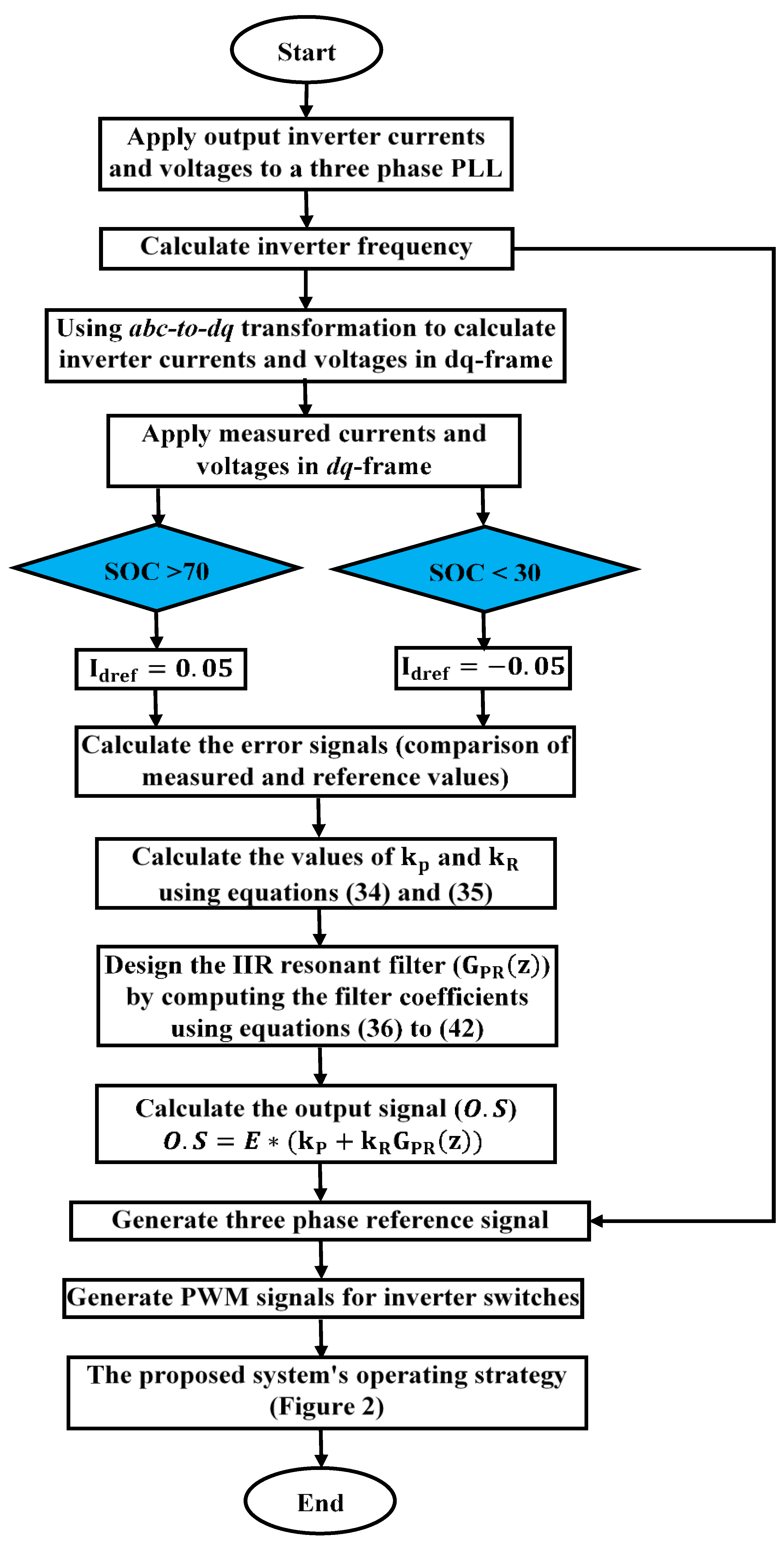
The mathematical modeling of the battery converter is described as follows:

$$V_D+V_{Bat}=L_3\frac{d{i}_{bat}}{dt}+R_3{i}_{bat}$$

(20)

$$V_D=V_d{D}_3$$

(21)

$$i_1\left(1-D_1\right)-i_b{D}_3-i_{AC}-i_{DC}=i_c=C_d\frac{d{V}_d}{dt}$$

(22)

where $D_3$ and $1-D_3$ denote the duty ratios of the converter switches, $V_D$ is the voltage of the center tap of the converter switches to ground, $L_3$ and $R_3$ are the converter’s main inductor and resistor, $i_{DC}$ is the DC bus current, and $V_{Bat}$ is the battery voltage.

3.6. DC/AC Inverter

The main converter’s AC side current equations are represented as follows in $dq$ coordinates:

$$C_2\frac{d}{dt}\left[\begin{array}{c}{V}_{sd}\\ V_{sq}\end{array}\right]=\left[\begin{array}{c}{I}_d\\ I_q\end{array}\right]+\left[\begin{array}{cc}0& \omega \\ -\omega & 0\end{array}\right]\left[\begin{array}{c}{v}_{sd}\\ v_{sq}\end{array}\right]-\left[\begin{array}{c}{i}_{od}\\ i_{oq}\end{array}\right]$$

(23)

The AC side voltage equations of the main inverter are shown in $abc$ and $dq$ coordinates, respectively, in Equations (24) and (25):

$$L_f\frac{d}{dt}\left[\begin{array}{c}{i}_a\\ i_b\\ i_c\end{array}\right]+R_f\left[\begin{array}{c}{i}_a\\ i_b\\ i_c\end{array}\right]=\left[\begin{array}{c}{v}_{Ca}\\ v_{Cb}\\ v_{Cc}\end{array}\right]-\left[\begin{array}{c}{v}_{C_{f}a}\\ v_{C_{f}b}\\ v_{C_{f}c}\end{array}\right]$$

(24)

$$L_f\frac{d}{dt}\left[\begin{array}{c}{I}_d\\ I_q\end{array}\right]=\left[\begin{array}{cc}-R_f& \omega L_f\\ -\omega L_f& -R_f\end{array}\right]\left[\begin{array}{c}{I}_d\\ I_q\end{array}\right]+\left[\begin{array}{c}{v}_{cd}\\ v_{cq}\end{array}\right]-\left[\begin{array}{c}{v}_{sd}\\ v_{sq}\end{array}\right]$$

(25)

where $i_{od}$ and $i_{oq}$ are the converter and transformer side $dq$-currents, respectively, $C_2$ is the inverter’s power filter capacitor, $R_f \mathrm{and} L_f$ are the inverter power filter resistor and inductor, $v_{Ca}, v_{Cb}, \mathrm{and} v_{Cc}$ are the voltages of AC side of inverter, $v_{C_{f}a}, v_{C_{f}b}, \mathrm{and} v_{C_{f}c}$ are the voltages across the capacitors of the three-phase power filter; I_d and I_q, $v_{cd} \mathrm{and} v_{cq}$, and $v_{sd} \mathrm{and} v_{sq}$ are the $dq$ coordinate variables that correspond to them.

4. The Converter Coordination Control

The hybrid MG employs distinct types of power converters. It is necessary to coordinate these converters with the utility grid in order to provide high-efficiency, uninterrupted, and high-quality power to the AC and DC loads. The boost converter’s control objective is to maintain the MPPT of the photovoltaic array by controlling its terminal voltage. The DFIG’s back-to-back AC/DC/AC converter has been controlled to obtain available power and synchronize with the AC grid. The hybrid grid’s excess energy can be sold to the utility grid. The battery’s primary purpose is to prevent frequent power transfer between both the DC and AC links. Using the technique in [46], the battery’s converter can be used as an energy buffer. The main converter is bidirectional in operation to take advantage of the complementary characteristics of wind and solar energy [47,48]. The main converter’s control objectives are to maintain a constant DC-link voltage for a DC load and to maintain synchronization with the utility system and the AC link.

As shown in Figure 1, the booster and main converter equivalent circuit models have been combined. The fundamental concepts and descriptions presented in the boosters and inverters sections in [49,50], respectively, served as the basis for this model. The following are the power flow equations for the DC and AC links:

$$P_{PV}+P_W=P_s+P_{AC,Load}+P_{DC,Load}+P_{Bat}$$

(26)

$$P_{AC}=P_W-P_s-P_{AC,Load}$$

(27)

where $P_{PV}$ and $P_W$ represent the real power generated by solar PV and WTG, respectively, $P_{AC,Load}$ and $P_{DC, Load}$ represent the active load powers of the AC bus and DC bus, $P_{AC}$ represents the power flow between the AC bus and DC bus, $P_{Bat}$ represents power injection to the battery, and $P_s$ represents power injection from the MG to the utility grid.

To maintain the hybrid MG running smoothly under different supply and demand scenarios, a coordination control algorithm is proposed for boost and main converters. This algorithm derives from the fundamental control algorithms of the grid-interactive inverter. The booster circuit’s control block diagram is shown in Figure 3. The basic P and O algorithm takes into account solar irradiance and temperature to establish a reference value for the terminal voltage $V_{PV}$ used by solar panels [51,52]. The PV system makes use of this control scheme so that the MPPT algorithm can maintain the optimum terminal voltage at the solar panels. The voltage loop based on the PI controller with proportional gain $k_p$ = 2 and integral gain $k_i$ = 0.2 is capable of ensuring tracking of the voltage reference with a zero error in steady state.

The battery’s energy constraints are determined by its $SOC$ limits, which are calculated as SOC_min < SOC ≤ SOC_max. It should be noted that while $SOC$ cannot be directly measured, it can be estimated using some of the methods described in [53,54]. The charging and discharging rates are constrained by $P_{Bat}\le P_{Bat,max}$. In the absence of the main grid, for cases of an idle battery or maximum power injection into the battery, either the PV system, the WTG, or both must operate in the off-MPPT mode; otherwise, either the PV system or the WTG must operate in the on-MPPT mode. For various situations, the battery buck-boost converter may operate in the discharging, charging, or idle mode by adopting the PI controller with proportional gain $k_p$ = 2 and integral gain $k_i$ = 0.2, as shown in Figure 3. If $P_w-P_{AC,Load}$ is negative, the inverter mode operation is the mode of operation of the main converter; if $P_w-P_{AC,Load}$ is positive, the converter mode operation is the operation mode of the main converter. When the battery has a low SOC and the electricity supply is lower than the demand, load shedding is required to keep the power grid stable.

To allow for a seamless exchange of power between DC and AC buses and the injection/withdrawal of a predetermined amount of power to/from the AC link (utility grid), a PR control is used to implement a current-controlled voltage source for the main converter. Two digital PR controllers are proposed for active and reactive power regulation, as shown in Figure 4. PR regulation regulates the DC bus voltage to keep it constant regardless of changes in load capacities or resource conditions. The PR controller is configured to serve as the instantaneous active current reference whereas the reactive power compensation command determines the instantaneous reactive current reference. As can be seen in Figure 4, the main inverter is controlled based on the SOC of the battery. In the case where the SOC is greater than 70%, the reference current along the d-axis is set to 0.5, and it is set to −0.5 for a SOC below 30%. The reference current along the q-axis set to 0. The measured values of the dq-frame currents and voltages are then applied to the current control block via two PR controllers to generate reference dq-frame voltages. All of the PR controller’s parameters can be calculated systematically. Equations (34)–(35) can be used to compute the controller gains, and the coefficients of the designed IIR filter can be calculated using Equations (35)–(42). The PR current controller output is converted from dq to abc frame using phase locked loop (PLL) frequency measurement. The final abc reference voltage is adopted to generate pulse width modulation (PWM) signals for inverter switches. This control method maintains system stability and allows the achievement of the power management strategy shown in Figure 2. The flowchart of the proposed control strategy is shown in Figure 5. When the DC load drops quickly and the DC side has more power than it needs, the main converter is turned on to move power from the DC side to the AC side. The capacitor’s active power consumption $C_d$ causes the DC-link voltage $V_d$ to rise. Through the PR control, the negative error ($V_d^{ref}-V_d$) caused by an increase in $V_d$ results in a higher active current reference $i_d^{ref}$. Both the active current $i_d$ and the reference $i_d^{ref}$ are positive. A higher positive reference current $i_d^{ref}$ forces an increase in active current $i_d$. As a result, the DC grid’s surplus power can be converted to the AC side. Similarly, the DC grid experiences a power outage and a drop in $V_d$ when the DC load suddenly increases. The principal converter is set up to provide electricity from the AC side to the DC side. The positive voltage error ($V_d^{ref}-V_d$) caused by $V_d$ drop increases the magnitude of $i_d^{ref}$ via the PR control. Due to the fact that $i_d$ and $i_d^{ref}$ are both negative, the magnitude of i_d increases. As a result, AC side-to-DC side power transfer occurs. The ideal PR controller’s transfer function is given as follows [55]:

$$G_{PRv}\left(s\right)=k_P+k_R\frac{s}{s^2+{\omega }_o^2}$$

(28)

where $k_P$ is the controller’s proportional gain, $k_R$ is the resonant gain of the controller, and ${\omega }_o$ is the resonant frequency, which is really the grid frequency.

Because it functions as an infinite quality factor system, the ideal PR controller is difficult to implement. As a result, the following is a nonideal PR controller transfer function [55]:

$$G_{PRv}\left(s\right)=k_P+k_R\frac{2{\omega }_{c}s}{s^2+2\zeta {\omega }_{c}s+{\omega }_o^2}$$

(29)

where ${\omega }_c$ denotes the bandwidth centers around the AC frequency ${\omega }_o$, and $\zeta$ denotes the damping factor.

Tustin’s method can be used to investigate analog controller discretization [56]. According to Equation (29), each S-domain component in analog controllers is replaced by a Z-domain (30).

$$s=\frac{z-1}{\frac{T}{2}\left(z+1\right)}$$

(30)

where T is the sampling period.

$$G_{PRv}\left(\frac{z-1}{\frac{T}{2}\left(z+1\right)}\right)=k_P+k_R\frac{2{\omega }_c\left(\frac{z-1}{\frac{T}{2}\left(z+1\right)}\right)}{{\left(\frac{z-1}{\frac{T}{2}\left(z+1\right)}\right)}^2+2\zeta {\omega }_c\left(\frac{z-1}{\frac{T}{2}\left(z+1\right)}\right)+{\omega }_o^2}=k_P+k_R{G}_{PR}\left(z\right)$$

(31)

The resonant path is defined by the Z-domain, which is cohesive with the gain $k_R$ and the resonant filter function $G_{PR}\left(z\right)$ given in Equation (32) [57,58].

$$G_{PR}\left(z\right)=\frac{b_0+b_1{z}^{-1}+b_2{z}^{-2}}{a_0+a_1{z}^{-1}+a_2{z}^{-2}}$$

(32)

where $b_0, b_1, b_2$ denote the feedback route parameters, and $a_0, a_1, a_2$ denote the feedforward route parameters of the filter. In Equation (32), the value of $a_0$ is deliberately set to 1 so that the difference equation can be written as follows:

$$y\left(n\right)=-a_{1}y\left(n-1\right)-a_{2}y\left(n-2\right)+b_{0}u\left(n\right)+b_{1}u\left(n-1\right)+b_{2}u\left(n-2\right)$$

(33)

where the resonance filter output is represented by $y\left(n\right)$, and the resonance filter input is represented by $u\left(n\right)$.

This is one of this work’s most significant contributions. The controller can use the resonant frequency to determine the frequency at which it should operate in order to obtain zero error in the steady state. When only the preferred filter frequency response in the S-domain is known, the designer can use it to compute the resonant filter coefficients using Tustin’s method, or the resonant gain, proportional gain, and filter coefficients can be determined using the Equations (34)–(42) [57].

$$k_p=\frac{\left(\sqrt{2\zeta +1}\right)(2\zeta +1){\omega }_r{L}_o-R_o}{V_{dc}}\frac{1}{H_i}$$

(34)

$$k_R=\frac{\left[{\left(2\zeta +1\right)}^2-1\right]{\omega }_r{}^2{L}_o}{2V_{dc}}\frac{1}{H_i}$$

(35)

where $H_i$ denotes the measured signal gain, $R_o$ and $L_o$ are the line resistor and inductor, respectively, and $V_{dc}$ is the DC input voltage of the inverter.

$$b_0=k_r{B}_r{T}_a$$

(36)

$$b_1=T_a\left[-k_r{B}_r{e}^{-0.5B_r{T}_a}\mathit{cos}\left(T_a\sqrt{{\omega }_r^2-\frac{1}{4}{B}_r^2}\right)-C\right]$$

(37)

where $C$ is a constant with the following definition:

$$C=\frac{0.5k_r{B}_r^2}{\sqrt{{\omega }_r^2-\frac{1}{4}{B}_r^2}}{e}^{-0.5B_r{T}_a}\mathit{cos}\left(T_a\sqrt{{\omega }_r^2-\frac{1}{4}{B}_r^2}\right)$$

(38)

$$b_2=0$$

(39)

$$a_0=1$$

(40)

$$a_1=-2e^{-0.5B_r{T}_a}\mathit{cos}\left(T_a\sqrt{{\omega }_r^2-\frac{1}{4}{B}_r^2}\right)$$

(41)

$$a_2=e^{-B_r{T}_a}$$

(42)

where ${\omega }_r$ denotes the angular frequency of the resonance, bandwidth $B_r$ is the angular resonant frequency, $T_a$ denotes the sampling time, and $k_r$ denotes the resonance gain.

The control parameters for the inverters used are listed in

Table 2. The control parameters of the main converters.

Parameter Name	Acronym	Value
bandwidth revolves around AC frequency ${\omega }_o$	${\omega }_c$	$2\left(3\right)\pi$
AC nominal frequency	${\omega }_r={\omega }_o$	$2\left(50\right)\pi$
Proportional gain PR current $dq$ compensator	$k_P$	0.3
Integral gain PR current $dq$ compensator	$k_R$	77
Damping coefficient PR current and power compensators	$\zeta$	0.95
Measured signal gain for DG1 and DG2	$H_i$	0.05
bandwidth revolves around AC frequency ${\omega }_o$	${\omega }_c$	$2\left(3\right)\pi$
AC nominal frequency	${\omega }_r={\omega }_o$	$2\left(50\right)\pi$

.

Table 3. The current loop PR resonant filter coefficients.

Coefficient	Value
$b_0$	8.682115835420001 × 10−6
$b_1$	0
$b_2$	−8.682115835420001 × 10−6
$a_0$	1
$a_1$	−1.999976025486589
$a_2$	0.999976124181453

contains the coefficients for the resonant filter portion of both PR controllers for two $dq$-axes current loops. Figure 6a illustrates the magnitude response of the designed resonant filter that was adopted in this study in the frequency domain. The only gain at a frequency of 50 Hz is equal to zero, demonstrating the effectiveness of the resonant filter. It is only necessary to multiply by one so the component of the error occurs at 50 Hz only. The power of all other error components has been significantly reduced. In addition, Figure 6a illustrates the phase response of the resonant filter, which is depicted at the bottom of Figure 6a. At resonance, the phase shift is 180 degrees due to the fact that both poles of the transfer function are in phase with one another. Figure 6b depicts the magnitude response of the PR controller that was designed. The frequency at which the greatest amount of amplification appears is 50 Hz. The phase response of the PR controller that was designed is depicted in the same figure. When low and high frequencies are being used, they have a phase that is as close as possible to zero.

Different control schemes for DFIGs, such as direct torque control (DTC) and direct power control (DPC), have been proposed in the literature [59,60]. In this paper, the DTC scheme is chosen as the rotor side converter’s control method. The rotational speed is determined by the wind turbine’s power and speed [61]. The electromagnetic torque is calculated using the rotational speed and mechanical power. It is possible to estimate the stator flux and use that information to compute the reference current for the $\mathrm{d}$-axis rotor side. By trying to adjust the corresponding current with proper feed-forward voltage compensation, the rotor side dq-voltages are kept stable.

5. Methodology of the ANNs

As indicated in [62,63], an ANN-based approach is among the most effective ones for detecting and localizing faults of AC grids and HVDC systems due to its accuracy, robustness, and quickness. The proposed control system used three ANN-based methods to detect, classify and localize faults in MGs, as shown in Figure 7. ANNs are information processing systems made up of linked neurons. These networks adapt their structure to forecast linear or nonlinear patterns in an external source (dataset).

A multilayer perceptron (MLP) network was employed in this investigation for the purposes of learning. The MLP network that has been constructed here employs a feed-forward strategy based on a supervised learning procedure to achieve its results. Unlike traditional networks where information is processed in both directions, a feed-forward network processes all information in just one direction, preventing feedback loops. Following processing by a layer of activation function, backpropagation is the way through which connection weights change in order to provide outputs for the following layer. According to the mean square error (MSE) value, this adjustment in the weights of the network is mathematically subjected to Equation (43) [64,65]:

$$MSE=\frac{0.5}{n}{\displaystyle \sum }_i^2{E}_i^2$$

(43)

where $n$ represents the total date number specified in a batch (epoch), and $E_i^2$ denotes the error value associated with the $i$-th data.

A supervised learning procedure was used to feed known input and desired values into the MLP network in order to anticipate the network’s outputs. Output and hidden layers contain activation functions (sigmoid and linear, respectively) that were used to generate/predict the dataset’s trend. The hidden layer’s activation function is a hyperbolic tan-sigmoid function defined across the range [−1, 1]. The output layer’s activation function is a linear function that enables linear mapping of the hidden layer results to the output of the network without defining restrictions. A linear function’s equation is the same as a straight line’s equation. As shown in Equation (44), a hyperbolic tangent equals a hyperbolic sine divided by a hyperbolic cosine [65].

$$f\left(x\right)=\frac{\mathit{sinh}(x)}{\mathit{cosh}(x)}=\frac{e^x-e^{-x}}{e^x+e^{-x}}$$

(44)

The MLP network was trained using the Levenberg–Marquardt (LM) method. The LM algorithm approach is considered superior to other algorithms in terms of performance because the changing learning rate can achieve optimal weights and low MSE [65,66]. The LM algorithm can be stated mathematically as:

$$\Delta w_m=\frac{d_m}{d_m^s+e^{\lambda }}$$

(45)

where $d_m$ is the error’s first derivative, $d_m^s$ is the error’s second derivative, and $\lambda$ is the damping factor.

The LM algorithm takes a combined Newtonian and gradient descent approach. The main goal is to minimize the total error by eliminating all gradients (first derivatives) [65].

The mathematical formulation for each neuron output in terms of updating the network’s weights ($w_i$) and bias ($b$) values are as follows:

$$S={\displaystyle \sum }_{i-1}^n\left(w_i\ast x_i\right)+b$$

(46)

The number of variables is denoted by $n$, and the weight given to each input value is indicated by $w_i$; $b$ stands for bias. Each batch of training data is used to fine-tune the weights and biases of the network until the MSE error rate is minimized. The training phase of the neural network is finished after that.

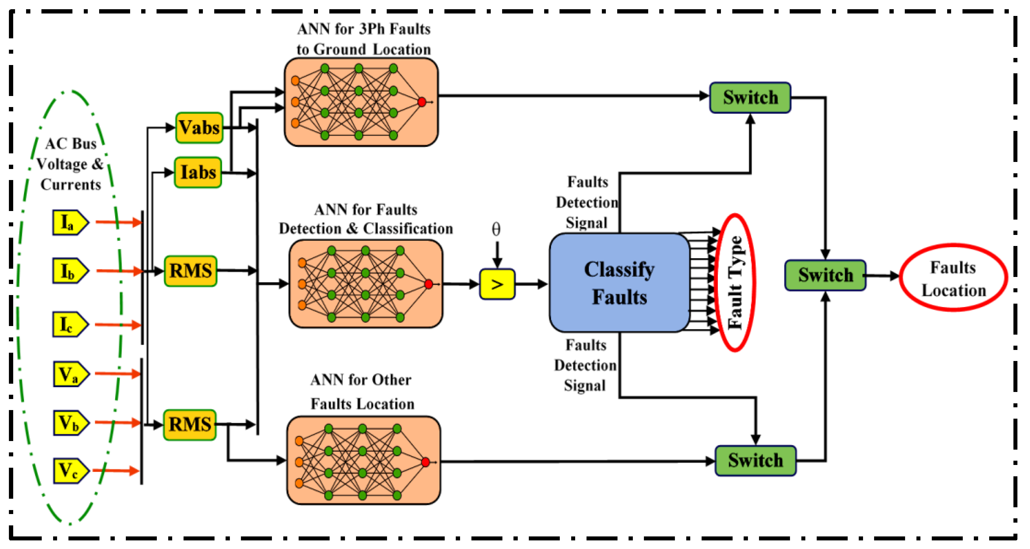
6. ANN-Based Fault Detection, Diagnostic, and Location

In the first step to apply neural networks in the adopted MG, useful statistical features are found in one cycle of postfault current and voltage signals from the sending end of the MG. It then normalizes the features and feeds them to the neural network as inputs. The MATLAB/Simulink program was used to run the simulation of the proposed technique under various loads and fault scenarios. In this study, using the neural network in an extreme learning machine, Figure 7 was generated in the MATLAB environment, allowing for fault detection, classification, and localization based on the following parameters: 70% (360 samples) values of the data were selected at random for real network training, 15% (54 samples) for data validation, and the remaining 15% (54 samples) for data testing.

The final ANN constructed for fault detection and classification has eight inputs, a single hidden layer containing 10 neurons, and five outputs. The eight inputs to the fault detection ANN are the three-phase root-mean-square values of the AC bus voltage and current and the magnitude of the sequence components specified. According to the three phase lines and ground line, the outputs consist of four nodes. The expected output for each line is “1” if a fault occurred and “0” otherwise. After creating the network architecture and sorting the raw data into the three categories below, ANN training began. Once the training phase was over and the resulting outputs were produced, they were compared to a threshold value and then classified logically using logic gates to determine the fault type.

The fault location was performed using two ANNs. The first one was used to locate the single line, double line, and triple line to ground faults. It had zero sequence current and voltage components as inputs and one output that indicates the distance. For all other faults, only the root mean square voltage of a three-phase AC bus served as adequate inputs to determine the location of these faults using another ANN.

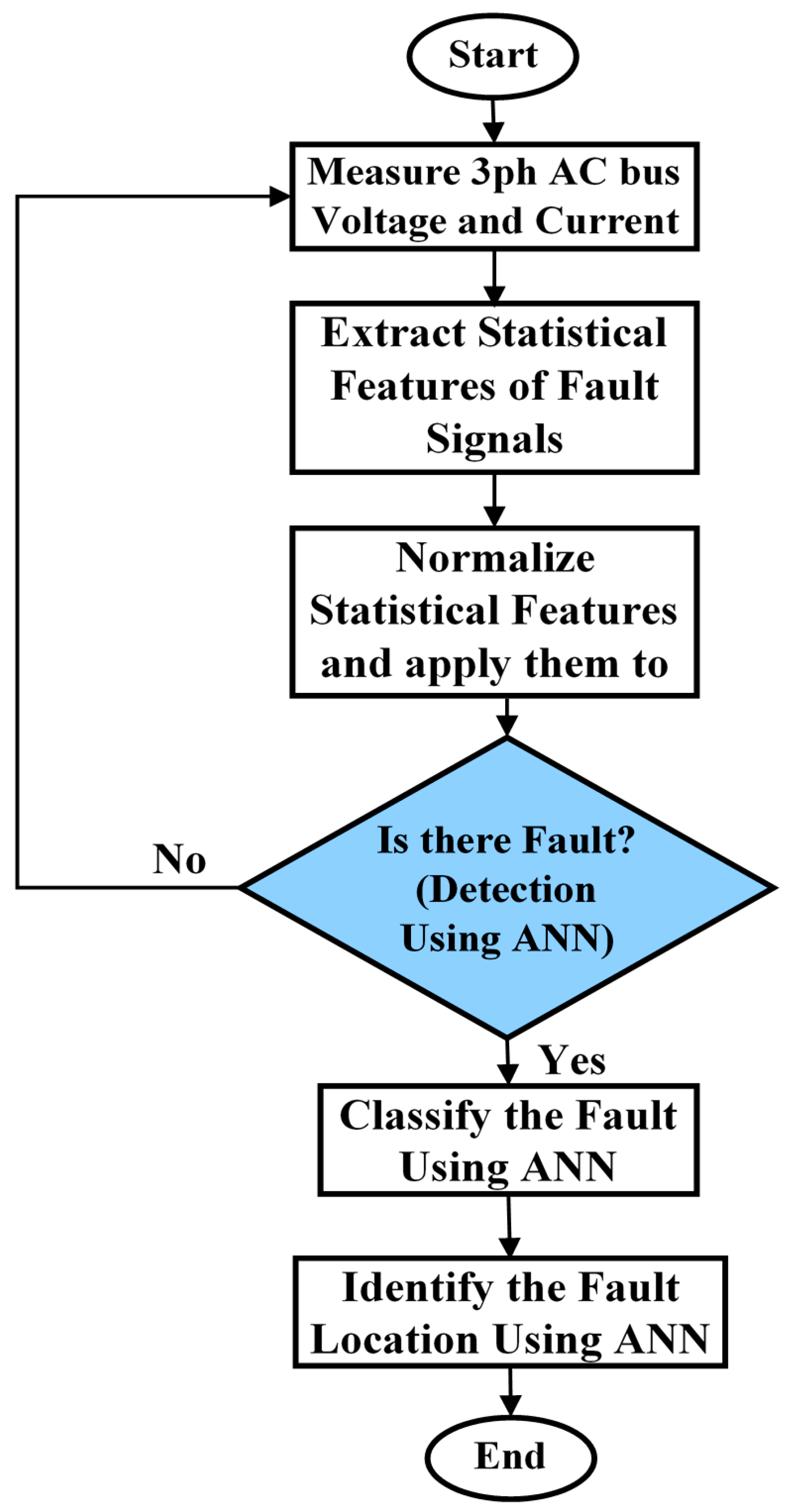
7. The Proposed ANN Process

The adopted inputs were applied to the designed ANN’s detection, classification, and location algorithm, which continuously monitors input status until a fault occurs. The AC bus generated output voltage and current waveforms, and these sine waves, which were then collected, constituted our raw data. This raw data underwent two significant data analysis steps: preprocessing and feature extraction. The raw fault data was cleansed, smoothed, and normalized during the data preprocessing phase to guarantee precise or meaningful analysis. The training data were then generated by extracting high-level features or attributes from the data. The model-building process then started with offline training and suitable tuning. For fault detection and classification-based ANNs, the training data passes through a feed-forward network consisting of an input layer, a hidden layer, and an output layer with 8-10-4 nodes configuration, respectively, and for three-phase faults to ground and other faults location-based ANNs, a 2-10-1 node configuration and 3-10-1 node configuration, respectively. The nodes determine the weight value of their incoming signal and output the weighted sum along with the result of the activation function. The outcome at the output node is the result of an open loop. The error, which is the difference between the desired outputs and the actual output, is backpropagated until it arrives at the hidden layer, at which point the weights are modified to reduce the error. This entire process is iterated for all training data until the error reaches a tolerable level, as rehiring the model using the same data typically improves the model. Back propagation-based ANN training uses the output to calculate weight changes. Backpropagation eliminates the constraint that related inputs lead to similar outputs in two-layer ANNs. Starting from the last step, each iteration and point’s error is calculated backward. Randomly choose weights for the neural network’s back-error-propagation algorithm, feedback them to an input pair, and obtain the result. After each step, the weights are updated, and the process is repeated for all inputs–outputs combinations in the developer’s training data set. This process continues until the network converges for the predefined target values and error tolerance. The proposed algorithm calculates each iteration’s error using MSE. The flow chart in Figure 8 illustrates the procedures for detecting, classifying, and localizing MG faults. The proposed ANN procedures can be divided into the following six steps:

• Three-phase current and voltage measurements on the AC side: One cycle of postfault current and voltage signals is taken for each phase at the line’s sending end of the MG.
• Extraction of statistical features: Statistical measures are applied to each voltage and current signal to extract statistical features, such as energy and root mean square values.
• The preceding two steps are repeated for various fault locations, fault types, and fault resistance values. Sufficient data must be generated in order for machine learning to be successful.
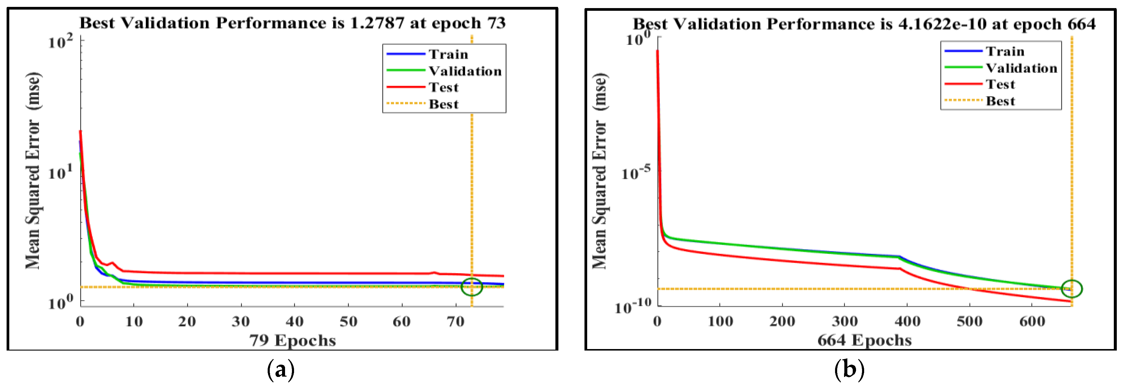
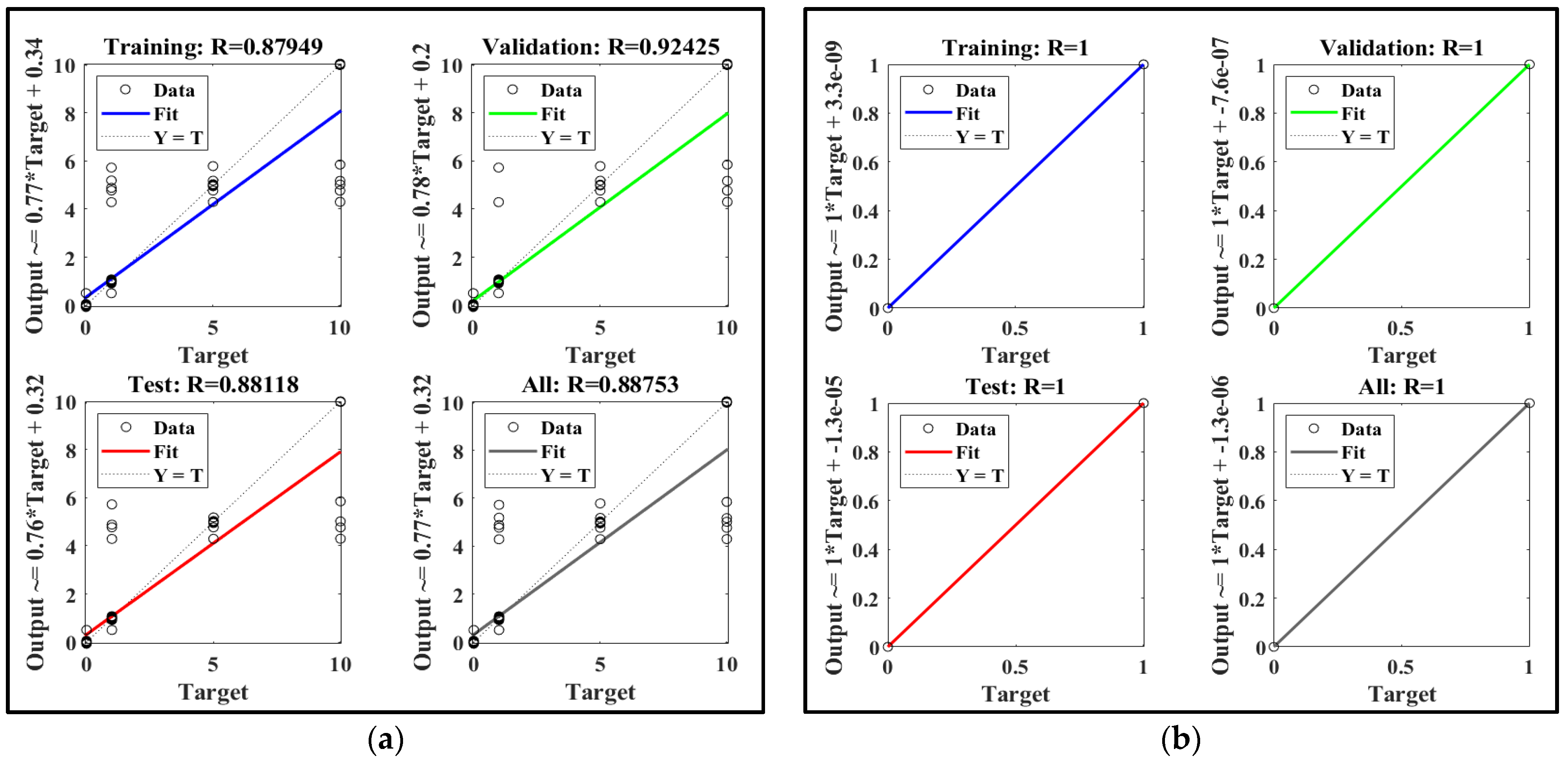
• Machine learning: The data generated is then used to train artificial neural networks for fault detection, classification, and localization purposes. The MLP network based on LM trained method is used for both detection and classification while the other two MLPs are used separately for fault location.
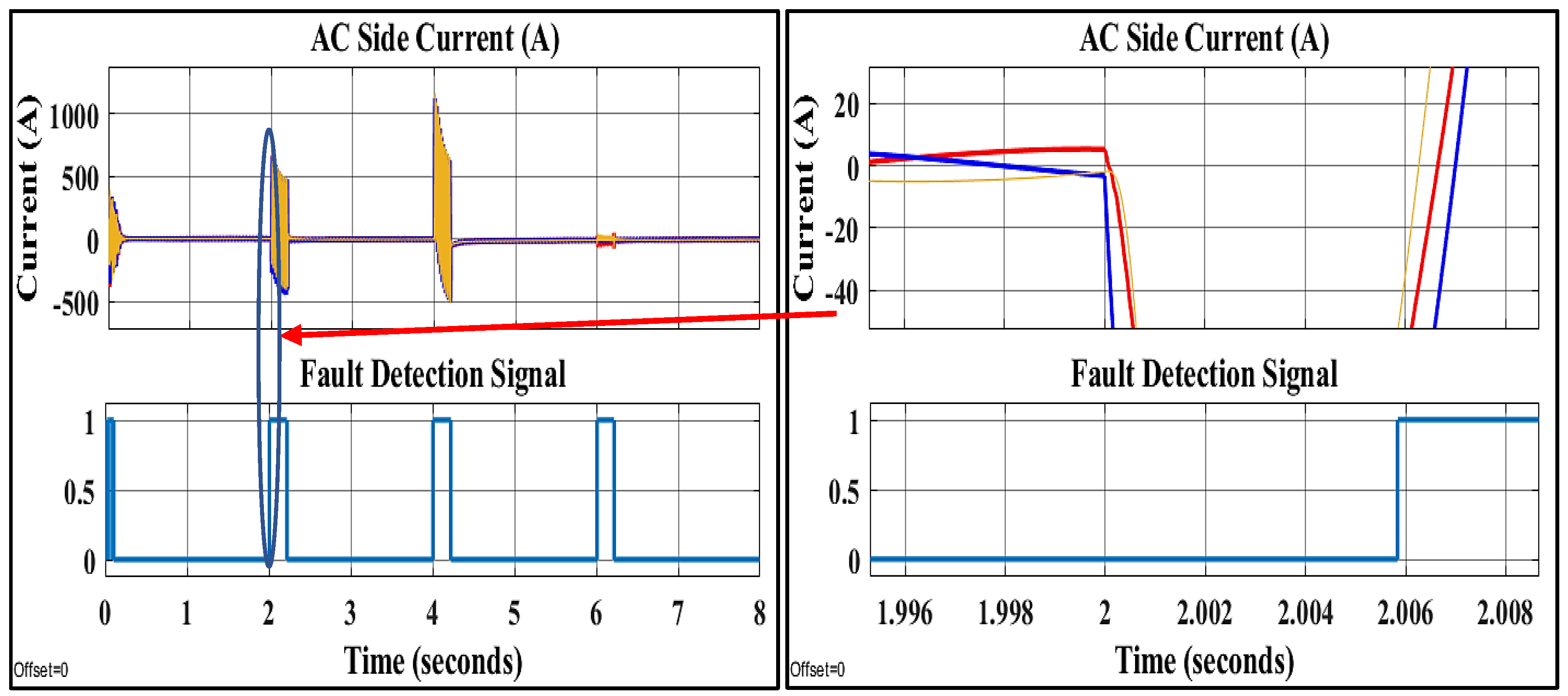
• Fault detection and identification: Once the machine learning algorithm has been adequately trained, it will be able to determine whether or not there is a fault.
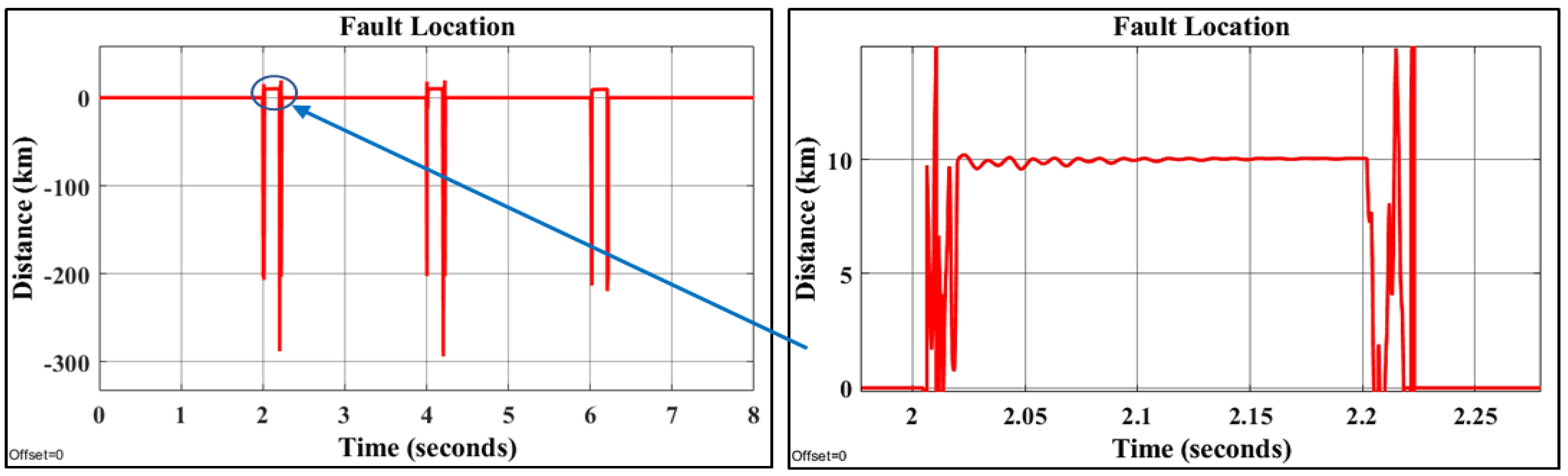
• Fault location: Once a fault has been detected and classified, its location is determined. The location is specified in terms of distance, which is determined by regression-based machine learning, whereas the type of fault is determined by classification-based machine learning.

8. Simulation Results

This study focuses on how the proposed hybrid AC/DC MG is operated properly in grid-connected mode by the proposed control technique and how the electrical power is exchanged between them for energy balance purposes as well as how faults are detected, classified, and localized using ANNs. Three different scenarios have been tested. In the first scenario, the PV generation changed, load demand changed in the second, and faults were applied in the third.

8.1. The First Scenario: Variations in Solar Irradiation

In the first scenario, the power of each renewable energy resource, grid, and the AC and DC loads are illustrated in Figure 9. It is evidenced that the adopted MG power is balanced under the solar irradiance variation according to Equations (26) and (27). It is evident that solar power is changed in accordance with solar irradiation variation. Variations in solar irradiance at intervals of 0, 1, 2, 3, 4, 5, 6, and 7 s are as follows: 1000, 800, 600, 400, 200, 0 (zero), 400, and 800 W/m². When solar irradiation decreases, the solar power decreases, and the battery power increases to meet the load demand while maintaining the system power balance. The reference DC voltage, measured voltage, current, and power of the DC bus are illustrated in Figure 10. Clearly, the measured DC bus voltage settles at 470 V, which is identical to the reference voltage. The DC bus power is 0.1 kW, which is the current multiplied by the voltage signal; it is exactly the same as the DC load power. Moreover, the buck-boost converter’s PI controller’s output signal along with the injected error signal is shown. Figure 11 illustrates the AC bus’s current and voltage. Regardless of the variability in PV generation, it is shown that the voltage and current are perfectly sinusoidal with constant magnitudes. The RMS current and voltage of the AC bus are shown in Figure 12a. It is clear that the voltage is at a nominal value (230 V) and the RMS current up to 4 A. As illustrated in Figure 12b, the AC bus operates at a nominal frequency of 50 Hz.

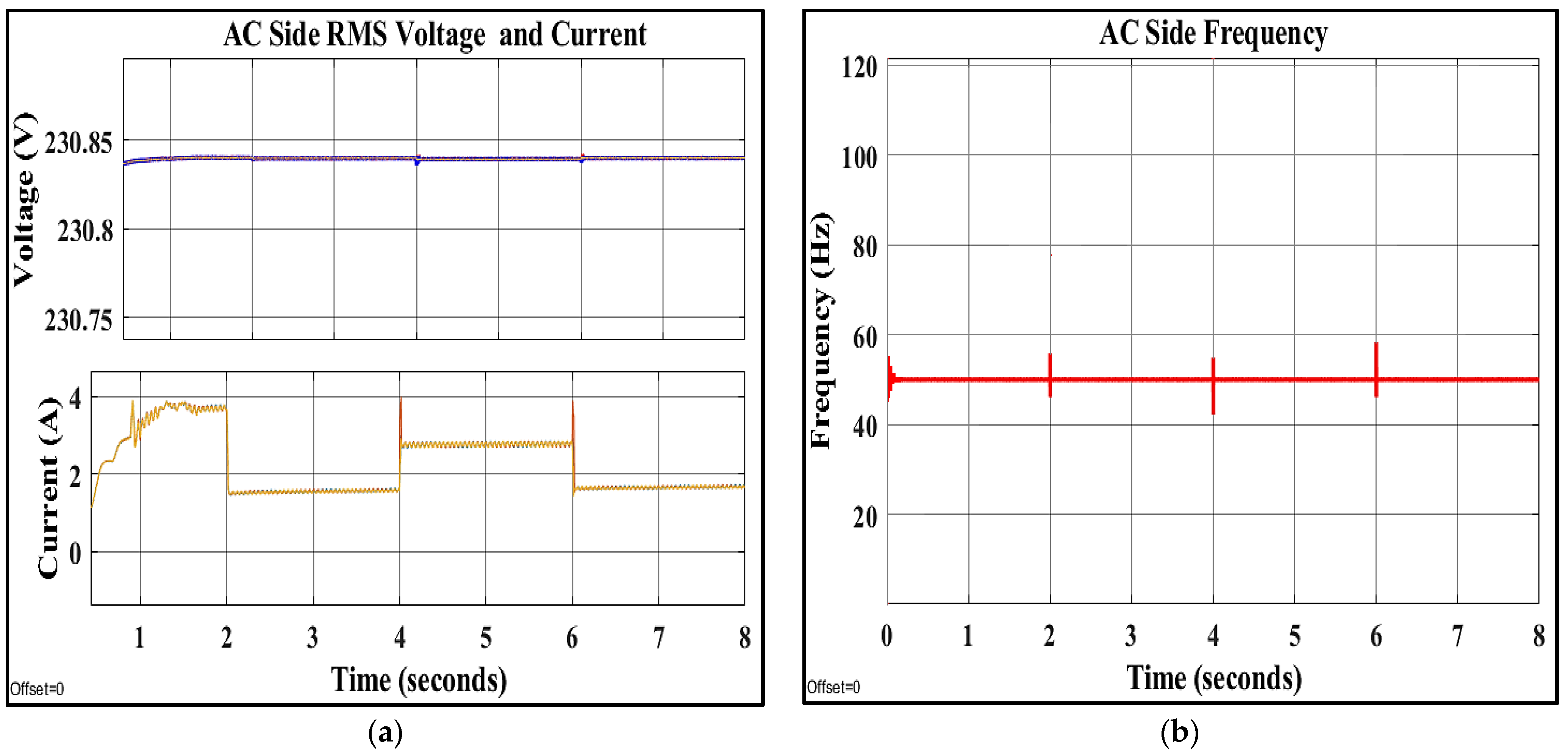
8.2. The Second Scenario: Variations in Load Demand

In the second scenario, the load has been changed as follows: Initially, the total AC loads consisted of two loads, which have respective powers of 0.4 kW and 0.25 kW. Then, the second one was increased to 2.25 kW, and then it was increased into 4.25 kW. Finally, it was returned to 2.25 kW. The power of each energy resource, grid, and the AC and DC loads are illustrated in Figure 13. The grid power was increased with the increasing load and vice versa to meet the load demand when the solar, wind, and battery power had insufficient power, so the utility grid compensated for the deficit. It is clear that the MG power is balanced under the load variation. At any point in time, the sum of solar and wind power minus load and battery power corresponds to excess power sold into the utility grid or required energy purchased from the main grid.

In this scenario, Figure 14 illustrates the current and voltage on the AC bus. As demonstrated in Figure 14, the current and voltage are pure sinusoidal signals with varying current signal magnitudes (when the load is increased, the magnitude decreases and vice versa). The RMS current and voltage are shown in Figure 15a. During load switching, the current is changed, and the RMS voltage is brought to its nominal value (230 V). As illustrated in Figure 15b, the AC bus operates at a nominal frequency of 50 Hz.

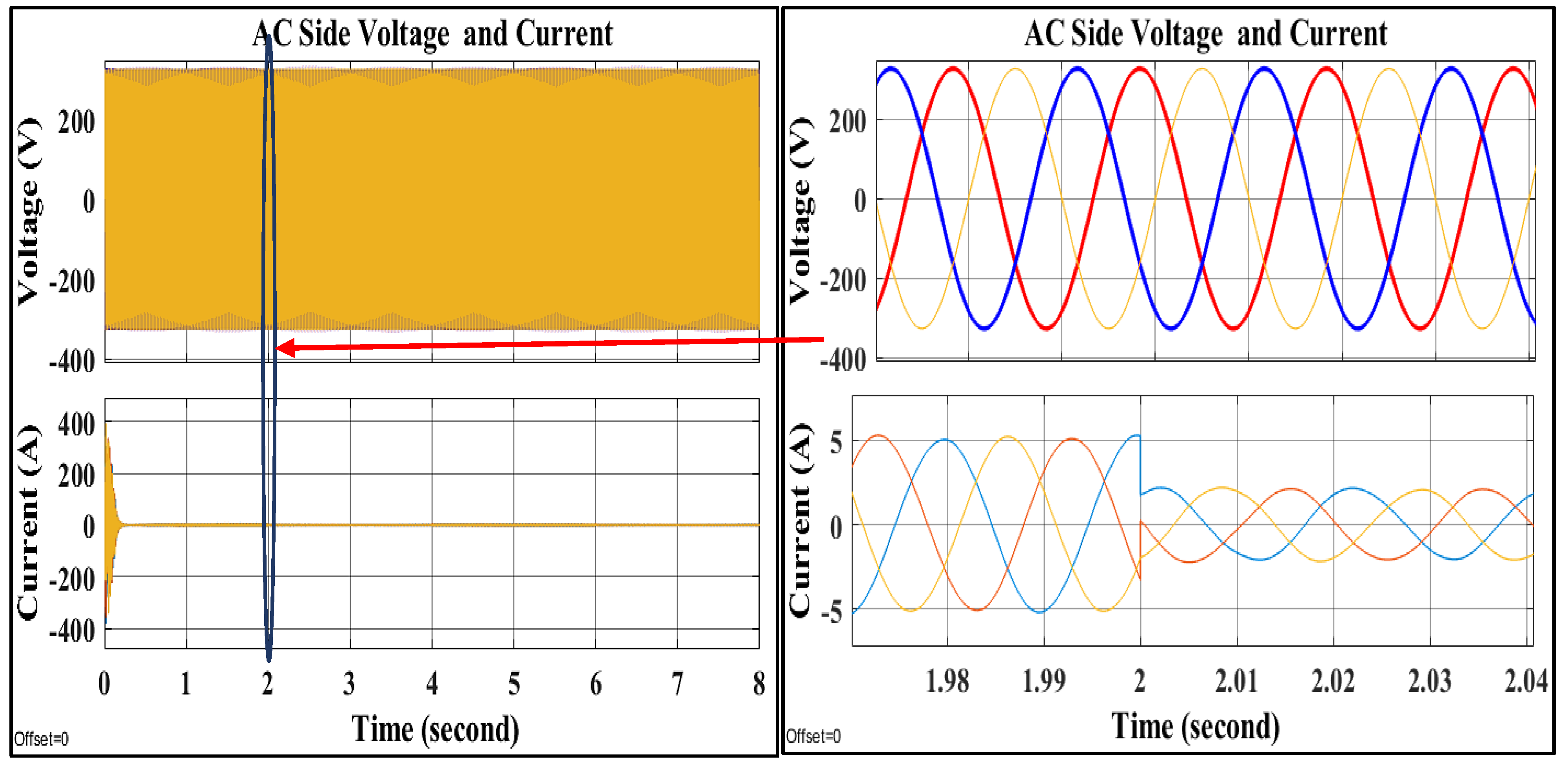
8.3. The Third Scenario: Applying Different Faults

The third scenario was used to test the proposed ANNs for detecting, classifying, and localizing three-phase faults. Suppose the proposed MG has experienced three-phase faults as follows: phase A to phase B to ground (ABG) fault, phase A to ground (AG) fault, and phase A to phase C (AC) fault at intervals [2 2.2] s, [4 4.2] s, and [6 6.2] s, respectively. The distance of the adopted AC line section is 5 km. Figure 16 makes it abundantly clear that the power of each energy source and load is kept at their respective nominal values during the intervals in which faults do not occur. Furthermore, one can observe that the system is balanced in accordance with Equations (26) and (27).

The fault detection and classification are shown in Figure 17. It is evident that the ABG, AG, and AC faults occur at time points of 2 s, 4 s, and 6 s, respectively, where the detector pulses are indicated by “1” for 0.2 s, which is the fault occurring time. Figure 18 illustrates the fault’s location, which occurs at a distance of 5 km. This is exactly because the AC line section length between the MG and the main grid is 5 km. In the second case of the scenario, the faults are located 10 km away, as illustrated in Figure 19. The AC bus current and voltage as well as the AC bus frequency are illustrated in Figure 20 and Figure 21, respectively. It can be seen that the three-phase current and voltage are pure sinusoidal signals with nominal values, and the frequency is also set at a nominal value (50 Hz). Figure 22 shows the fault detection signal and AC bus current. Clearly, the time required to detect the fault by ANN is 0.00058 s. This is a very short and accepted time period for detecting a fault. Moreover, the fault location determined by the ANN is widely accepted with a time period of 0.02 s, as shown in Figure 23.

As shown in Figure 24a,b, the best validation performance for fault classification and detection is 1.2787 at epoch 73 while it is 4.1622 × 10⁻¹⁰ at epoch 664 for fault location. The MSE is the square root of the average difference between outputs and targets. Reduced values are preferable while zero indicates no error [67]. Figure 24 depicts the variation in validation, training, and test errors as a function of the number of training epochs. The graph shows the network’s MSE beginning at a large value and gradually decreasing to a smaller value, indicating that the network learned properly. As the weights improve, the error in the training set decreases. After 73 and 664 epochs, respectively, training was halted when the validation error began to increase. This result is reasonable because the final MSE is small, the error characteristics of the test and validation sets are similar, and no significant overfitting occurred at 73 and 664 epochs, respectively.

Figure 25 depicts a regression analysis with validation, training, and test data for fault detection and classification in (a) and the fault’s location in (b). The dashed line represents the ideal line on which the targets and outputs are equal. Points of data are depicted by the circles while the colored line indicates the best outputs-to-targets fit. The circles congregate across the dashed line, indicating that the outputs are relatively close to the targets. As a result of these findings, it can be concluded that the ANN structure is adequate for fault prediction. Figure 25b shows that the colored line is exactly on the dashed line, indicating that there is no error and that the output is equal to the target data.

9. Conclusions

This paper proposed a hybrid AC/DC grid connected-MG to minimize the number of power electronic conversions. Coordination control has been presented to maximize the power generated by renewable energy resources; coordinate power flow between AC and DC buses; and ensure both the AC and DC buses’ stability under changeable demand/supply conditions. This study proposed a discrete PR controller-based coordination control mechanism for the MG main inverter. The procedure for designing discrete PR controllers is described in detail. The resonant and proportional gains along with the coefficients of the digital resonant IIR filter have been computed using a systematic approach. The main advantages of the proposed method are that it mitigates the increasing instability caused by high penetration rates of renewable energy by maintaining a balance between consumption demand and production levels, it is implemented in a discrete time domain, and it can be easily created due to the systematic nature of its parameter selection procedure. In addition to being accurate, reliable, and fast, this method also adopted an ANN to create a smart online fault detection, diagnostic, and localization information system for hybrid low-voltage AC/DC MGs. This study used an MLP network to learn. The LM method was used to train the MLP network. The LM algorithm is preferred over competing algorithms due to its ability to optimize weights via changes in the learning rate, resulting in lower MSE values. MATLAB/Simulink was adopted to simulate the proposed MG and observe the system performance. The results demonstrated that the system is capable of maintaining a perfect power balance within the system with total generation power being equal to total consumption. The DC bus voltage was measured to have stabilized at 470 V while the AC bus operates at a nominal frequency of 50 Hz and 230 V RMS voltage. Moreover, the proposed method of fault detection and location only needs 0.00058 s for the ANN to detect the fault. It is a standardized, relatively accepted time period for fault detection. The 0.02 s time frame that the ANN uses to pinpoint the source of a malfunction is also widely accepted. However, since the proposed discrete control relies on an IIR digital filter, it requires more computations and significantly more processing time than analog methods. Because of this, a fast processor with a high sampling frequency is required for implementation.

References

1. Jasim, A.M.; Jasim, B.H.; Mohseni, S.; Brent, A.C. Consensus-based dispatch optimization of a microgrid considering meta-heuristic-based demand response scheduling and network packet loss characterization. Energy AI 2023, 11, 100212. [Google Scholar] [CrossRef]
2. Kroposki, B.; Lasseter, R.; Ise, T.; Morozumi, S.; Papathanassiou, S.; Hatziargyriou, N. Making microgrids work. IEEE Power Energy Mag. 2008, 6, 40–53. [Google Scholar] [CrossRef]
3. Behera, C.K.; Thakur, A.K.; Singh, S.P. P-Q Controller of Grid-Connected Microgrid with Smart Inverter Based PV Distributed Energy Resources. In Proceedings of the 2020 International Conference on Electrical and Electronics Engineering (ICE3), Gorakhpur, India, 14–15 February 2020. [Google Scholar]
4. Etemadi, A.H.; Davison, E.J.; Iravani, R. A Generalized Decentralized Robust Control of Islanded Microgrids. IEEE Trans. Power Syst. 2014, 29, 3102–3113. [Google Scholar] [CrossRef]
5. Levron, Y.; Guerrero, J.M.; Beck, Y. Optimal Power Flow in Microgrids with Energy Storage. IEEE Trans. Power Syst. 2013, 28, 3226–3234. [Google Scholar] [CrossRef] [Green Version]
6. Corchero, C.; Cruz-Zambrano, M.; Heredia, F.J. Optimal energy management for a residential microgrid including a vehicleto-grid system. IEEE Trans. Smart Grid 2014, 5, 2163–2172. [Google Scholar]
7. Paudyal, S.; Canizares, C.A.; Bhattacharya, K. Optimal Operation of Industrial Energy Hubs in Smart Grids. IEEE Trans. Smart Grid 2015, 6, 684–694. [Google Scholar] [CrossRef]
8. Pedrasa, M.A.A.; Spooner, T.D.; MacGill, I.F. Coordinated Scheduling of Residential Distributed Energy Resources to Optimize Smart Home Energy Services. IEEE Trans. Smart Grid 2010, 1, 134–143. [Google Scholar] [CrossRef]
9. Kerekes, T.; Teodorescu, R.; Rodriguez, P.; Vazquez, G.; Aldabas, E. A New High-Efficiency Single-Phase Transformerless PV Inverter Topology. IEEE Trans. Ind. Electron. 2011, 58, 184–191. [Google Scholar] [CrossRef] [Green Version]
10. Jasim, A.M.; Jasim, B.H.; Bureš, V. A novel grid-connected microgrid energy management system with optimal sizing using hybrid grey wolf and cuckoo search optimization algorithm. Front. Energy Res. 2022, 10, 960141. [Google Scholar] [CrossRef]
11. Jena, S.; Babu, C.; Mishra, G.; Naik, A. Reactive power compensation in inverter-interfaced distributed generation. In Proceedings of the 2011 International Conference on Energy, Automation, and Signal (ICEAS), Bhubaneswar, India, 28–30 December 2011; pp. 1–6. [Google Scholar]
12. Hornik, T.; Zhong, Q.-C. A Current-Control Strategy for Voltage-Source Inverters in Microgrids Based on H∞ and Repetitive Control. IEEE Trans. Power Electron. 2011, 26, 943–952. [Google Scholar] [CrossRef]
13. Jeong, H.-G.; Kim, G.-S.; Lee, K.-B. Second-Order Harmonic Reduction Technique for Photovoltaic Power Conditioning Systems Using a Proportional-Resonant Controller. Energies 2013, 6, 79–96. [Google Scholar] [CrossRef]
14. Jasim, A.M.; Jasim, B.H.; Neagu, B.-C. A New Decentralized PQ Control for Parallel Inverters in Grid-Tied Microgrids Propelled by SMC-Based Buck–Boost Converters. Electronics 2022, 11, 3917. [Google Scholar] [CrossRef]
15. Zakzouk, N.E.; Abdelsalam, A.K.; Helal, A.A.; Williams, B.W. High Performance Single-Phase Single-Stage Grid-Tied PV Current Source Inverter Using Cascaded Harmonic Compensators. Energies 2020, 13, 380. [Google Scholar] [CrossRef] [Green Version]
16. Xie, B.; Guo, K.; Mao, M.; Zhou, L.; Liu, T.; Zhang, Q.; Hao, G. Analysis and Improved Design of Phase Compensated Proportional Resonant Controllers for Grid-Connected Inverters in Weak Grid. IEEE Trans. Energy Convers. 2020, 35, 1453–1464. [Google Scholar] [CrossRef]
17. James, J.Q.; Hou, Y.; Lam, A.Y.; Li, V.O. Intelligent Fault Detection Scheme for Microgrids with Wavelet-Based Deep Neural Networks. IEEE Trans. Smart Grid 2017, 10, 1694–1703. [Google Scholar]
18. Zhang, F.; Mu, L. A Fault Detection Method of Microgrids with Grid-Connected Inverter Interfaced Distributed Generators Based on the PQ Control Strategy. IEEE Trans. Smart Grid 2018, 10, 4816–4826. [Google Scholar] [CrossRef]
19. Jena, P.; Pradhan, A.K. Directional relaying during single-pole tripping using phase change in negative-sequence current. IEEE Trans. Power Deliv. 2013, 28, 1548–1557. [Google Scholar] [CrossRef]
20. Liu, K.; Li, Y. Study on solutions for active distribution grid protection. Proc. CSEE 2014, 34, 2584–2590. [Google Scholar]
21. Borghetti, A.; Bosetti, M.; Nucci, C.A.; Paolone, M.; Abur, A. Integrated Use of Time-Frequency Wavelet Decompositions for Fault Location in Distribution Networks: Theory and Experimental Validation. IEEE Trans. Power Deliv. 2010, 25, 3139–3146. [Google Scholar] [CrossRef]
22. He, Z.; Zhang, J.; Li, W.-H.; Lin, X. Improved Fault-Location System for Railway Distribution System Using Superimposed Signal. IEEE Trans. Power Deliv. 2010, 25, 1899–1911. [Google Scholar] [CrossRef]
23. Jafarian, P.; Sanaye-Pasand, M. A Traveling-Wave-Based Protection Technique Using Wavelet/PCA Analysis. IEEE Trans. Power Deliv. 2010, 25, 588–599. [Google Scholar] [CrossRef]
24. Lin, Y.-H.; Liu, C.-W.; Yu, C.-S. A new fault locator for threeterminal transmission lines using two-terminal synchronized voltage and current phasors. IEEE Trans. Power Deliv. 2002, 17, 452–459. [Google Scholar]
25. Al Hassan, H.A.; Reiman, A.; Reed, G.F.; Mao, Z.H.; Grainger, B.M. Model based fault detection of inverter based microgrids and a mathematical framework to analyse and avoid nuisance tripping and blinding scenarios. Energies 2018, 11, 2152. [Google Scholar] [CrossRef] [Green Version]
26. Hare, J.; Shi, X.; Gupta, S.; Bazzi, A. Fault diagnostics in smart micro-grids: A survey. Renew. Sustain. Energy Rev. 2016, 60, 1114–1124. [Google Scholar] [CrossRef]
27. Fahim, S.R.; Sarker, Y.; Islam, O.K.; Sarker, S.K.; Ishraque, M.F.; Das, S.K. An Intelligent Approach of Fault Classification and Localization of a Power Transmission Line. In Proceedings of the 2019 IEEE International Conference on Power, Electrical, and Electronics and Industrial Applications (PEEIACON), Dhaka, Bangladesh,, 29 November–1 December 2019; pp. 53–56. [Google Scholar]
28. Fahim, S.R.; Sarker, Y.; Sarker, S.K.; Sheikh, M.R.I.; Das, S.K. Self attention convolutional neural network with time series imaging based feature extraction for transmission line fault detection and classification. Electr. Power Syst. Res. 2020, 187, 106437. [Google Scholar] [CrossRef]
29. Al-Nasseri, H.; Redfern, M.; Li, F. A voltage based protection for micro-grids containing power electronic converters. In Proceedings of the 2006 IEEE Power Engineering Society General Meeting, Montreal, QC, Canada, 18–22 June 2006; p. 7. [Google Scholar]
30. Rengaraj, R.; Venkatakrishnan, G.R.; Shalini, S.; Subitsha, R.; Suganthi, S.; Carolyn, S.S. Identification and classification of faults in underground cables—A review. IOP Conf. Ser. Mater. Sci. Eng. 2021, 1166, 012018. [Google Scholar] [CrossRef]
31. Shi, Q.; Kanoun, O. Wire Fault Diagnosis in the Frequency Domain by Impedance Spectroscopy. IEEE Trans. Instrum. Meas. 2015, 64, 2179–2187. [Google Scholar] [CrossRef]
32. Naval, K.; Prabhat, K. Distribution System Fault Detection and Classification using Wavelet Transform and Artificial Neural Networks. In Proceedings of the 11th IOE Graduate Conference Peer Reviewed 2022, Pokhara, Nepal, 10–11 March 2022; Venue: Paschimanchal Campus, IOE, TU. Volume 11, pp. 10–11. [Google Scholar]
33. Chen, K.; Huang, C.; He, J. Fault detection, classification and location for transmission lines and distribution systems: A review on the methods. High Volt. 2016, 1, 25–33. [Google Scholar] [CrossRef]
34. Bunnoon, P. Fault Detection Approaches to Power System: State-of-the-Art Article Reviews for Searching a New Approach in the Future. Int. J. Electr. Comput. Eng. (IJECE) 2013, 3, 553–560. [Google Scholar] [CrossRef]
35. Musa, M.H.; He, Z.; Fu, L.; Deng, Y. A correlation coefficientbased algorithm for fault detection and classification in a power transmission line. IEEJ Trans. Electr. Electron. Eng. 2018, 13, 1394–1403. [Google Scholar] [CrossRef]
36. Ponukumati, B.K.; Sinha, P.; Maharana, M.K.; Jenab, C.; Kumar, A.P.; Akkenaguntla, K. Pattern Recognition Technique Based Fault Detection in Multi-Microgrid. In Proceedings of the 2nd International Conference on Applied Electromagnetics, Signal Processing, & Communication, Bhubaneswar, India, 26–28 November 2021; pp. 1–6. [Google Scholar] [CrossRef]
37. De La Ree, J.; Centeno, V.; Thorp, J.S.; Phadke, A.G. Synchronized Phasor Measurement Applications in Power Systems. IEEE Trans. Smart Grid 2010, 1, 20–27. [Google Scholar] [CrossRef]
38. Fahim, S.R.; Datta, D.; Sheikh, M.R.I.; Dey, S.; Sarker, Y.; Sarker, S.K.; Badal, F.R.; Das, S.K. A Visual Analytic in Deep Learning Approach to Eye Movement for Human-Machine Interaction Based on Inertia Measurement. IEEE Access 2020, 8, 45924–45937. [Google Scholar] [CrossRef]
39. Sarker, Y.; Fahim, S.R.; Sarker, S.K.; Badal, F.R.; Das, S.K.; Mondal, M.N.I. A Multidimensional Pixel-wise Convolutional Neural Network for Hyperspectral Image Classification. In Proceedings of the 2019 IEEE International Conference on Robotics, Automation, Artificial-intelligence and Internet-of-Things (RAAICON), Dhaka, Bangladesh, 29 November–1 December 2019; pp. 104–107. [Google Scholar]
40. Fahim, S.R.; Sarker, Y.; Rashiduzzaman, M.; Islam, O.K.; Sarker, S.K.; Das, S.K. A Human-Computer Interaction System Utilizing Inertial Measurement Unit and Convolutional Neural Network. In Proceedings of the 2019 5th International Conference on Advances in Electrical Engineering (ICAEE), Dhaka, Bangladesh, 26–28 September 2019; pp. 880–885. [Google Scholar]
41. Casagrande, E.; Woon, W.L.; Zeineldin, H.H.; Svetinovic, D. A Differential Sequence Component Protection Scheme for Microgrids with Inverter-Based Distributed Generators. IEEE Trans. Smart Grid 2014, 5, 29–37. [Google Scholar] [CrossRef]
42. Che, L.; Khodayar, M.E.; Shahidehpour, M. Adaptive Protection System for Microgrids: Protection practices of a functional microgrid system. IEEE Electrif. Mag. 2014, 2, 66–80. [Google Scholar] [CrossRef]
43. Jamalaldin, S.; Hakim, S.; Razak, H. Damage Identification Using Experimental Modal Analysis and Adaptive Neuro-Fuzzy Interface System (ANFIS). In Topics in Modal Analysis, Conference Proceedings of the Society for Experimental Mechanics Series 30; Springer: New York, NY, USA, 2012; Volume 5, pp. 399–405. [Google Scholar]
44. Zhi, D.; Xu, L. Direct power control of DFIG with constant switching frequency and improved transient performance. IEEE Trans. Energy Conv. 2007, 22, 110–118. [Google Scholar] [CrossRef]
45. Tremblay, O.; Dessaint, L.-A.; Dekkiche, A.-I. A Generic Battery Model for the Dynamic Simulation of Hybrid Electric Vehicles. In Proceedings of the IEEE Vehicle Power and Propulsion Conference, Arlington, TX, USA, 9–12 September 2007; pp. 284–289. [Google Scholar]
46. Bo, L.; Shahidehpour, M. Short-term scheduling of battery in a grid-connected PV/battery system. IEEE Trans. Power Syst. 2005, 20, 1053–1061. [Google Scholar]
47. Daniel, S.; AmmasaiGounden, N. A Novel Hybrid Isolated Generating System Based on PV Fed Inverter-Assisted Wind-Driven Induction Generators. IEEE Trans. Energy Convers. 2004, 19, 416–422. [Google Scholar] [CrossRef]
48. Wang, C.; Nehrir, M.H. Power Management of a Stand-Alone Wind/Photovoltaic/Fuel Cell Energy System. IEEE Trans. Energy Convers. 2008, 23, 957–967. [Google Scholar] [CrossRef]
49. Lin, J.L.; Chang, C.H. Small-signal modeling and control of ZVT-PWM boost converters. IEEE Trans. Power Electron. 2003, 18, 2–10. [Google Scholar]
50. Sozer, Y.; Torrey, D.A. Modeling and Control of Utility Interactive Inverters. IEEE Trans. Power Electron. 2009, 24, 2475–2483. [Google Scholar] [CrossRef]
51. Kroutikova, N.; Hernandez-Aramburo, C.; Green, T. State-space model of grid-connected inverters under current control mode. IET Electr. Power Appl. 2007, 1, 329–338. [Google Scholar] [CrossRef] [Green Version]
52. Liu, F.; Duan, S.; Liu, F.; Liu, B.; Kang, Y. A variable step size INC MPPT method for PV systems. IEEE Trans. Ind. Electron. 2008, 55, 2622–2628. [Google Scholar]
53. Anbuky, A.; Pascoe, P. VRLA battery state-of-charge estimation in telecommunication power systems. IEEE Trans. Ind. Electron. 2000, 47, 565–573. [Google Scholar] [CrossRef]
54. Kutluay, K.; Cadirci, Y.; Ozkazanc, Y.S.; Cadirci, I. A new online state-of-charge estimation and monitoring system for sealed lead-acid batteries in telecommunication power supplies. IEEE Trans. Ind. Electron. 2005, 52, 1315–1327. [Google Scholar] [CrossRef]
55. Cha, H.; Vu, T.K.; Kim, J.E. Design and Control of Proportional-Resonant Controller Based Photovoltaic Power Conditioning System. In Proceedings of the 2009 IEEE Energy Conversion Congress and Exposition, IEEE Xplore, San Jose, CA, USA, 20–24 September 2009. [Google Scholar]
56. Shabib, G.; Abd-Elhameed, E.H.; Magdy, G. A New Approach to the Digital Implementation of Analog Controllers for a Power System Control. Int. J. Sci. Eng. Res. 2014, 5, 419–427. [Google Scholar]
57. Busarello TD, C.; Pomilio, J.A.; Simoes, M.G. Design Procedure for a Digital Proportional-Resonant Current Controller in a Grid Connected Inverter. In Proceedings of the 2018 IEEE 4th Southern Power Electronics Conference (SPEC), in IEEE Xplore, Singapore, 10–13 December 2018. [Google Scholar]
58. Jasim, A.; Mahmood, J.; Salim, R. Design and Implementation of a Musical Water Fountain Based on Sound Harmonics Using IIR Filters. Int. J. Comput. Digit. Syst. 2020, 9, 319–333. [Google Scholar]
59. Arnalte, S.; Burgos, J.C.; Rodríguez-Amenedo, J.L. Direct Torque Control of a Doubly-Fed Induction Generator for Variable Speed Wind Turbines. Electr. Power Compon. Syst. 2002, 30, 199–216. [Google Scholar] [CrossRef]
60. Kim, W.S.; Jou, S.T.; Lee, K.B.; Watkins, S. Direct power control of a doubly fed induction generator with a fixed switching frequency. In Proceedings of the 2008 IEEE Industry Applications Society Annual Meeting, Edmonton, AB, Canada, 5–9 October 2008; pp. 1–9. [Google Scholar]
61. Koutroulis, E.; Kalaitzakis, K. Design of a maximum power tracking system for wind-energy-conversion applications. IEEE Trans. Ind. Electron. 2006, 53, 486–494. [Google Scholar] [CrossRef]
62. Mirzaei, M.; Ab Kadir MZ, A.; Moazami, E.; Hizam, H. Review of fault location methods for distribution power system. Aust. J. Basic Appl. Sci. 2009, 3, 2670–2676. [Google Scholar]
63. Jasim, A.M.; Jasim, B.H.; Bureš, V.; Mikulecký, P. A New Decentralized Robust Secondary Control for Smart Is-907 landed Microgrids. Sensors 2022, 22, 8709. [Google Scholar] [CrossRef]
64. Aggarwal, L.; Aggarwal, K.; Urbanic, R.J. Use of artificial neural networks for the development of an inverse kinematic solution and visual identification of singularity zone(s). Procedia CIRP 2014, 17, 812–817. [Google Scholar] [CrossRef]
65. Samarsinghe, S. Neural Networks for Applied Sciences and Engineering; Auerbach Publications: Boca Raton, FL, USA, 2006. [Google Scholar]
66. Souza, C.D. Neural Network Learning by the Levenberg-Marquardt Algorithm with Bayesian Regularization (Part 1). Available online: https://www.codeproject.com/Articles/55691/Neural-Network-Learningby-the-Levenberg-Marquardt (accessed on 6 October 2022).
67. Al-Shayea, Q.K. Artificial neural network in medical diagnosis. Int. J. Comput. Sci. 2011, 8, 150–154. [Google Scholar]
Figure 1. A diagrammatic illustration of the proposed hybrid AC/DC MG.
Electronics 12 00187 g001
Figure 2. The proposed system’s operating strategy.
Electronics 12 00187 g002
Figure 3. The block diagram of circuits and control mechanism of the booster and buck-boost converters.
Electronics 12 00187 g003
Figure 4. The control diagram of the main converter.
Electronics 12 00187 g004
Figure 5. The flowchart of the proposed control strategy.
Electronics 12 00187 g005
Figure 6. The magnitude and phase response of the adopted (a) resonance filter and (b) PR controller.
Electronics 12 00187 g006
Figure 7. ANN-based schematic representation for fault detection, classification, and location.
Electronics 12 00187 g007
Figure 8. Flowchart for fault detection, classification, and location using ANNs.
Electronics 12 00187 g008
Figure 9. The power of generation resources, main grid, and AC and DC loads under the first scenario.
Electronics 12 00187 g009
Figure 10. DC bus readings measured with input and output of the PI controller in (Scenario 1).
Electronics 12 00187 g010
Figure 11. AC bus current and voltage 3ph signals (Scenario 1).
Electronics 12 00187 g011
Figure 12. 3Ph AC bus RMS current and voltage in (a) and frequency in (b) under first Scenario 1.
Electronics 12 00187 g012
Figure 13. The power of generation resources, main grid, and AC and DC loads under load variation.
Electronics 12 00187 g013
Figure 14. Three-phase AC bus current and voltage.
Electronics 12 00187 g014
Figure 15. AC bus RMS current and voltage in (a) and frequency in (b).
Electronics 12 00187 g015
Figure 16. The power of each RER, grid, and AC and DC loads under fault scenario.
Electronics 12 00187 g016
Figure 17. Fault detection and classification.
Electronics 12 00187 g017
Figure 18. Fault location (Scenario 3, Case 1).
Electronics 12 00187 g018
Figure 19. Fault location (Scenario 3, Case 2).
Electronics 12 00187 g019
Figure 20. Three-phase AC bus current and voltage under fault conditions.
Electronics 12 00187 g020
Figure 21. AC bus frequency under faults occur.
Electronics 12 00187 g021
Figure 22. AC bus current and fault detection signal.
Electronics 12 00187 g022
Figure 23. AC bus current and fault location signal.
Electronics 12 00187 g023
Figure 24. The evolution of training, validation, and test errors for (a) fault classification and detection and (b) fault location.
Electronics 12 00187 g024
Figure 25. ANN regression graphs with training and test sets for (a) fault detection and classification, and (b) fault location.
Electronics 12 00187 g025