
A Powered Floor System with Integrated Robot Localization

Department of Engineering and Architecture, University of Trieste, 34127 Trieste, Italy
*
Author to whom correspondence should be addressed.
Electronics 2023, 12(1), 234; https://doi.org/10.3390/electronics12010234
Submission received: 22 November 2022
/
Revised: 23 December 2022
/
Accepted: 26 December 2022
/
Published: 3 January 2023
(This article belongs to the Special Issue Intelligent Control and Application for Robotics)
Abstract
:One of the most pressing issues in the field of mobile robotics is power delivery. In the past, we have proposed a powered floor based solution. In this article, we propose a system which combines a powered floor with a robot pose estimation system. The floor on which the mobile robots stand is composed of an array of interdigitated conductors that provide DC power supply; the stripes of conductors are interwoven similarly to what happens in a carpet, thus creating a sort of checkerboard of positive and negative pads. The robots are powered through sliding contacts. The power supply voltage is modulated with a binary encoding that uniquely identifies each conductor stripe power line; in this way, each robot is able to self-localize, by exploiting the information coming from the contacting pins. We describe the theoretical framework that allows concurrent power delivery and localization (with error boundaries). Then, we present the experimental evaluation that we performed using a prototype realization of the proposed powered floor system.
1. Introduction
Delivering electrical power to mobile robots or, more generally, to mobile systems is a challenge in many operative fields: transportation, automation, and logistics. Power supply systems based on sliding contacts [1] are an effective solution to power a large number of mobile robots, especially in swarm robotics applications, where powering a single robot by manually recharging the battery is time-consuming. They are also simple to implement and inexpensive. Usually the floor is made up of interdigitated stripes; these are positive and negative conductors. Mobile robots are equipped with a series of pins (sliding contacts) in contact with either the floor conductors or the insulator. The condition for the robot to be powered is that at least one pin has to be in contact with a positive voltage stripe and at least another pin has to be in contact with a negative voltage stripe. Multiple pins could be in contact with positive or negative conductors. Also, it may happen that some pins are in contact with the insulating band that is interposed between a positive and a negative conductor. Typically, the conducting stripes are arranged parallel to each other; their size is chosen according to the number of pins and their distance from the center of the robot.
In this work, we propose to exploit the powered floor not only to deliver power but also to communicate with the robot in order to provide localization information; i.e., we employ a one-way communication from the ground transmitter to the robot. Indeed, the powerline communication problem has been solved since the early 70 with the definitions of well-known protocols, such as X10. The main contribution and the innovative aspect of our work is the presence of a large number of communication lines (robot contact points), that can deliver power and signal data at the same time.
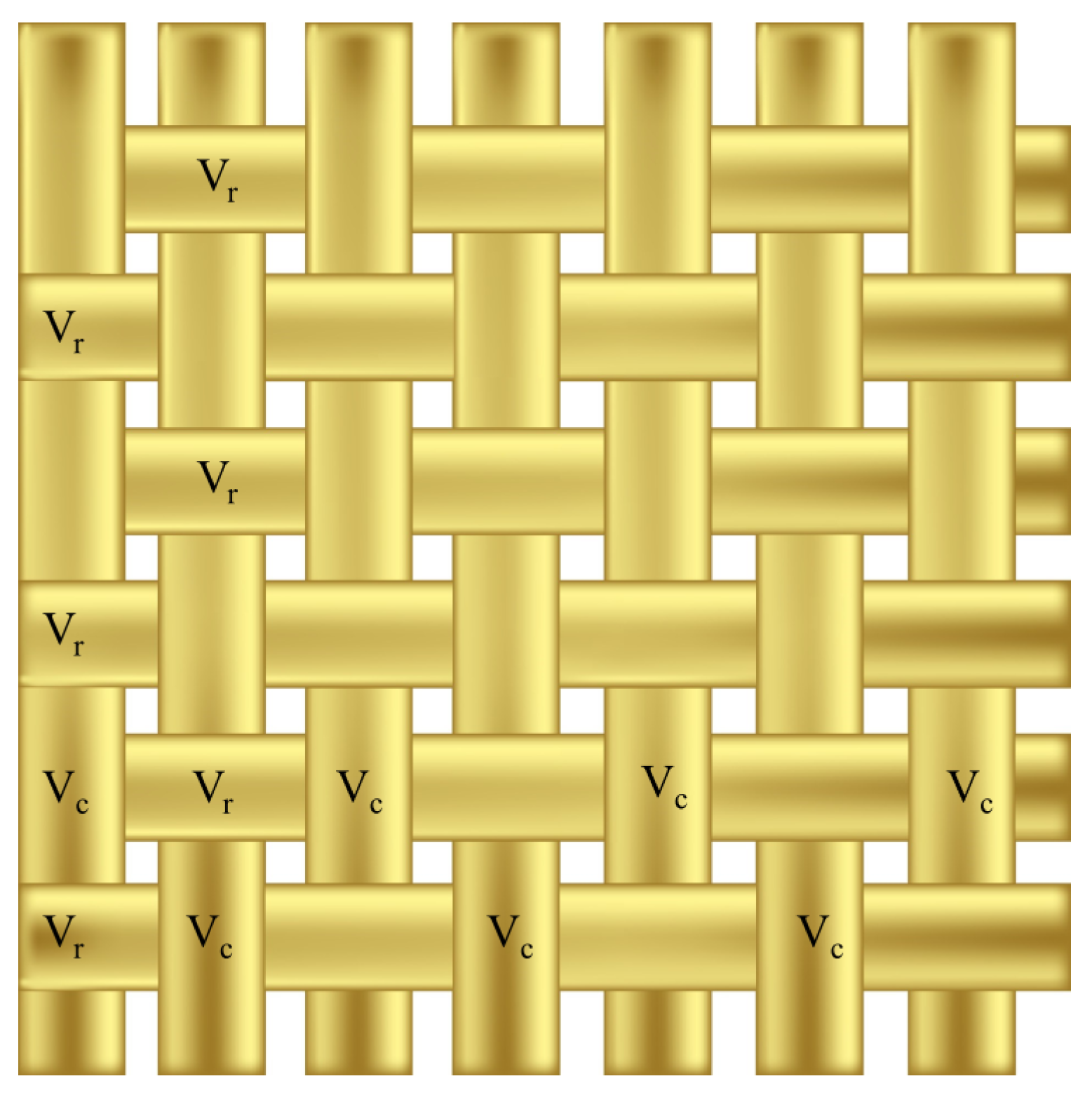
More in detail, power lines are intertwined as shown in Figure 1, so that the exposed areas, which we call pads, are arranged such as in a chessboard. Horizontal stripes (the rows) are powered with the voltage, while vertical stripes (the columns) are powered with the voltage. The power sent on these lines is modulated according to a simple binary Pulse Width Modulation (PWM), which is used to provide position information to each row or column of the chessboard. Indeed, we use several simultaneous transmission lines; each robot uses the modulated signals to compute its own pose by means of a localization algorithm. The higher the number of pins in contact, the more accurate the localization algorithm.
We think that our proposed system may be of particular interest for practitioners who need to experiment with several mobile robots at the same time, possibly by performing long-lasting experiments in which human intervention would be costly. Other ways exist for powering mobile robots and localizing them at the same time, but they often pose constraints on the environment or on the robotic platforms, hence limiting the practical applicability. E.g., vision-based localization system require proper lighting conditions, cable-based power supply systems may limit the mobility of robots, battery-based systems require service stops for charging. An example of use case where our proposed architecture may prove beneficial is experimentation in promiscuous environments, i.e., where robots and humans coexist. In this setting, overhead monitoring may fail due to being partially occluded by individuals, while position determination performed at floor-level would not. This case can be extended to the case where human agents are “simulated” by other robots. Our system explores a different trade-off between applicability, cost, and effectiveness. By tolerating some decrease in localization accuracy (for which we provide, though, an upper bound), the practitioner can easily set up a setting suitable for long, unattended experiments with mobile robots.
Powered Floor State of the Art
Traditionally, electrical mobility of robots relies on batteries. This is the standard for road transportation, logistics (Autonomous Ground Vehicles, AVGs), and general purpose mobile robots [2]. The most common solution that does not involve the use of energy storage comes for railway technologies: electrified railroad systems employ sliding contacts mounted on pantographs. In this way the aerial cable conductors close the electrical circuit with the conducting rails [3,4]. Less common and more complex solutions are conductors embedded in the road, introduced for the Ansaldo-Breda project TramWave [5].
AVGs are becoming increasingly popular in the manufacturing industry for logistics applications or, to a lesser extent, for re-positioning manipulators or other automated systems. These robotic systems entirely rely on batteries for their power supply; thanks to this solution, no external infrastructure is required. Conversely, expensive and time-consuming downtime due to charge time is necessary [6,7]. As a consequence, study projects have been conducted in order to find alternative powering strategies [8]. The most common approach found in mobile robots literature is that of wireless energy delivery through the use of resonant inductive coupling [9,10]. A similar approach has been employed in the field of electrical road transportation [11,12,13,14]. Thanks to the intensive development of research in these areas, comparative studies and surveys have also been carried out [15,16,17]. In particular, Jang et al. discuss on the current state-of-the-art of these systems. They pointed out that the benefits of distribution without the need for energy storage are innumerable; however, the costs associated with the necessary infrastructure are still too expensive for large-scale distribution. In fact, wireless power transfer systems require arrays of coils for the transmitter placed throughout the entire floor and produce very high values of stray magnetic fields [15]. Other approaches rely on the logistics of power delivery, rather than on the technology itself; two main areas of investigation are coordinated charging [18] and energy logistics models [19]. For niche applications, special situations where batteries cannot be used and where movement areas are confined, tethered-based power systems have been studied [20,21].
For applications in which a large number of small mobile robots are used, a common way of delivering energy to mobile robots is by means of sliding contacts [22,23]. For this reason, swarm robotics is a field which shows remarkable affinity with the concept of powered floors [24,25,26]. In general, this type of power delivery system allows for relative motion in a single direction, as is the case with slip-rings. However, some examples have been proposed that allow for bi-dimensional relative motion; in 2002, Watson et al. [27] apply a methodology—originally invented by C. Shannon at the AT&T Bell Laboratories in 1950—for continuous power delivery to small mobile swarm robots: this was based on sliding contacts. Another interesting example is the Droplets platform [28].
Powered floors may be particularly beneficial when robots have to be optimized automatically for performing a given task through a trial-and-error process, as in evolutionary robotics [29] or reinforcement learning [30]. By relying on powered floors, researchers can run long-time experiments involving real robots, without the need to pause or stop the experiment to change them. Using real robots is a key strategy for fighting the reality gap problem [31,32] that makes solutions obtained by optimization in simulation far from being optimal when ported in reality.
Ultimately, the application is key in the correct determination of the more suitable type of powered floor. All other solutions (e.g., batteries, tethers, etc.) mentioned up to this point tend to severely hinder the freedom of movement of the vehicles, and are thus ill-suited either for continuous operation or in cluttered environments.
One key aspect in mobile robotics is almost invariably that of robot localization or position determination, i.e., the set of techniques used to determine the configuration of the robot with respect to an inertial global frame of reference. Several techniques exist and are used in various kinds of operating conditions on mobile robots. For a very broad overview on position determination see the recent work from Alatise et al. [33]. The most general classification is between relative and absolute positioning [34]. Methods pertaining to the former determine position relative to the robot frame, and are usually self-contained on the agent itself; the most common example of these are odometric methods, which integrate wheels rotations or acceleration data to infer the past trajectory of the robot [35]; another relative positioning method is Simultaneous Localization And Mapping (SLAM) [36]. Conversely, absolute positioning, most notably represented by Global Navigation Satellite Systems (GNSSs), determines the pose of the robot relative to a fixed reference frame [37]. For fleets of small robots, a promising approach is that of distributed radiofrequency (RF) range-finding and triangulation [38]. A schematic summary of the main techniques is shown in Table 1.
In a previous paper [1], we focused on a systematic study of the alternating bands sliding-contact based powered floor introduced by C. Shannon in the 1950s [27]; we provided a comprehensive framework for contact patterns for robots, based on regular polygons of n sides. In particular we demonstrated that triangle- and rectangle-shaped patterns cannot always guarantee contact, and that Shannon’s pattern itself has several limitations.
The major disadvantage of the solution we proposed in [1] is that, although each robot is autonomous in terms of power, it is not able to determine its own pose and localization. Therefore, an additional localization system is necessary (optical system, LIDAR, etc.). To solve this problem, we have conceived, designed, and tested a special floor that can simultaneously provide electric power and information for the self-localization of each robot. This solution is particularly advantageous in scenarios where a large number of robots are involved (e.g., swarm robotics), or in cluttered or promiscuous environments.
The paper is organized as follows. In Section 2, we present a comprehensive analysis of the concept of chessboard powered floor, along with the main factors that we will take into consideration in the rest of the article. In particular, we introduce a metric to evaluate the robot’s power supply efficiency, intended as the ratio between the set of all the poses in which the robot is effectively powered and the set of all the possible poses reachable by the robot. In Section 3, we present the detailed design of the prototype. In Section 4, we present an experimental campaign to validate both the power supply mechanism and the localization. Finally, in Section 5 we present our concluding remarks.
2. Theoretical Framework
The geometry of the contact pads and of the polarity stripes deeply influences the performance of the powered floor and of the delivery system in general, i.e., the functionality and robustness of the system.
As mentioned in the introduction, the system provides two services: it delivers power to the robot, and allows the robot to localize itself (i.e., to estimate its position and rotation). Regarding the first function, it is necessary to optimize the contact pin configuration of the robot. In particular, we developed a theoretical framework to solve this problem: what is the optimal combination of the number of contact pins and their distance from the robot center that allows the robot to be powered with the highest efficiency? Hence, in order to provide the means for a quantitative approach to the problem, we propose a general framework for the computation of the performance and we introduce an index of efficiency. As far as the localization is concerned, we present an algorithm that, based on the proposed design for the powered floor, allows the robot to estimate its position within a predefined error range.
2.1. Power Supply Framework
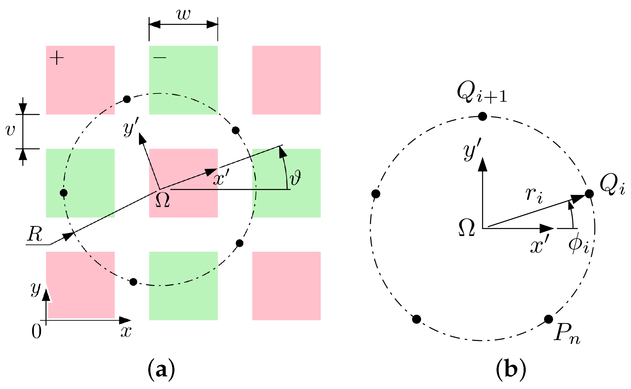
Figure 2 graphically represents the mathematical framework of the contact problem. The squares represent the planar conducting pads arranged in a checkered pattern whose side is w: the same voltage is provided to all the pink squares; moreover, a common voltage is provided to the green ones. and are assigned in such a way that , where is the voltage necessary to power the robot. The squares are separated by non-conducting narrow stripes. is the geometric center of the robot, is the inertial reference frame, is the frame linked to the robot, while is the angular orientation of the robot. We call pose the 2-ple representing the position and rotation of the robot.
The robot is provided with n sliding contacts , named pins in the following, that power the robot circuitry. and are the polar coordinates of the i-th pin with respect to the robot reference frame. The sliding contacts are placed on a circumference, thus all the are equal. What it is relevant to the problem is the position of each pin, namely:
Without loss of generality, let’s assume that the origin of the inertial frame is located at the corner of a pink square, as in figure. Therefore an interval of coordinates that bounds a square area is given by the set:
where l and m are positive integers that sequentially identify the squares. Therefore the whole area with voltage is identified by
At the same time, the area with voltage is identified by
In other words, is the union of the squares for which the sum of l and m is an even number. Conversely, is the union of the squares for which the sum of l and m is an odd number.
In order to define when a pin is in contact with or pad, let’s define the functions:
Therefore, when the i-th pin is powered by a voltage , the Boolean value of is 1 (true), otherwise 0 (false). Likewise, when the i-th pin is powered by a voltage , the Boolean value of is true. Note that for all i. Given the robot geometric parameters , and for a given robot pose , the power supply module is powered when a pin i exists for which and, at the same time, another pin j exists (with ) for which . Mathematically, this is expressed by the function:
where and . A value guarantees power supply for a given pose of the robot on the floor. In order for the robot to reach every point of the working space without losing power supply, it is necessary that on the entire space. We can define the function,
where and represent all the possible robot poses on the floor. In conclusion, a robot with pins position given by is powered for each pose on the floor only if the following equation is verified:
It is rather difficult to achieve the efficiency imposed by Equation (10); in general this requires to have a large number of contact pins, which complicates the electromechanical realization of the robot. It has to be noted, however, that most mobile robots have backup batteries. Therefore, it is not necessary for the robot to be powered in all the points of a trajectory, but only in most of them. Therefore, instead of ensuring a pin configuration that guarantees that the robot will be powered for every pose, it is better to look for a compromise that balances power efficiency with design simplicity. For this reason, we introduce another index which provides an indication of power supply efficiency:
is in the range . If , then, for every pose of the robot, there is always at least one pin in contact with pad and at least one pin in contact with a pad.
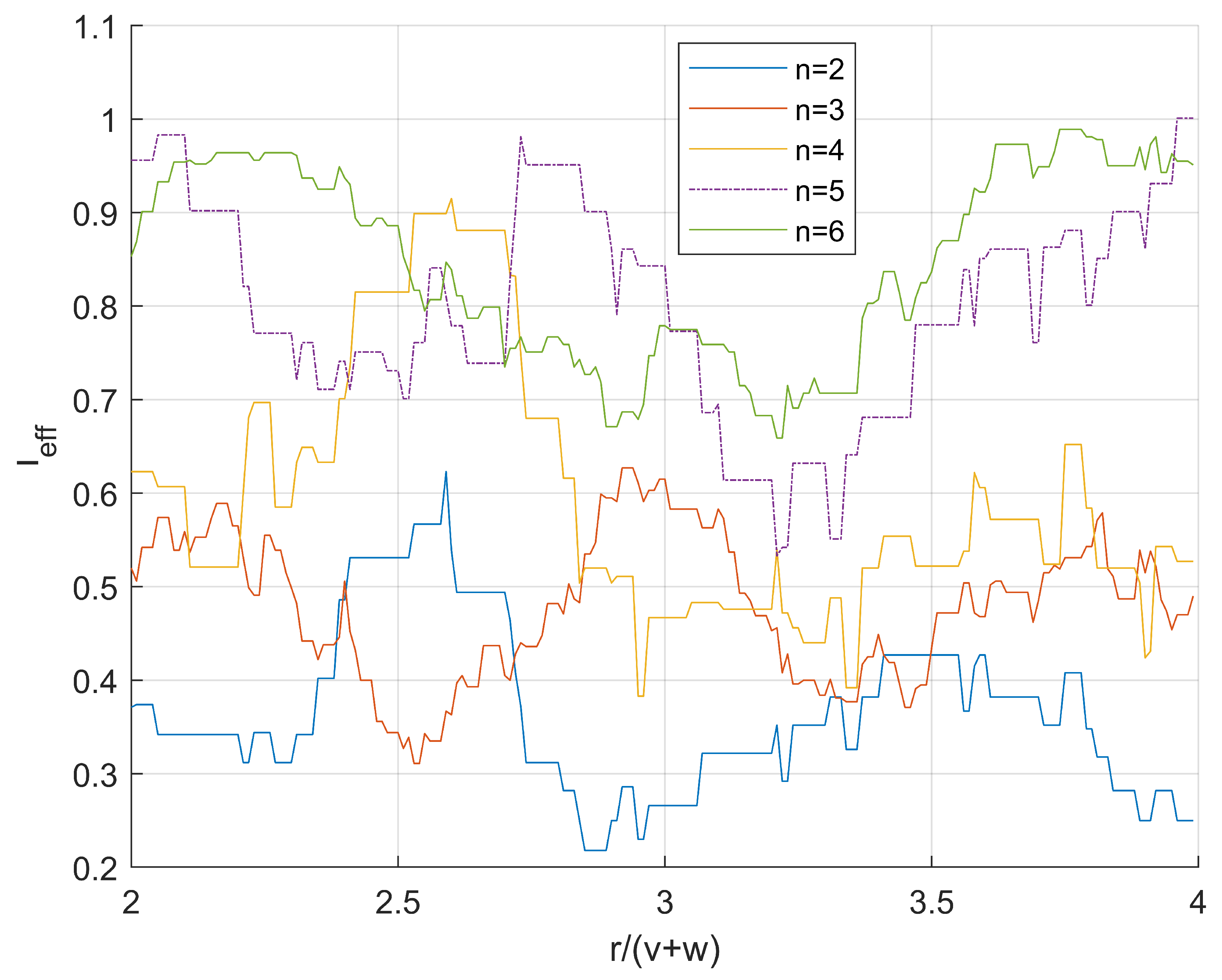
The value of depends – in a non-trivial way – by the design of the powered floor system, i.e., on v, w, r, and the number n of pins in the robot. Figure 3 shows, for different values of n (line color), the values of vs. (the relative radius). As one can notice, a value of is reached with a configuration of at least 5 pins and a relative radius of almost 4.
The robot we are going to use to verify the theory is a differential wheeled robot Thymio-II, model 2AFKS-WLTHYMIO (http://www.thymio.it/, accessed on 28 January 2022). The footprint of the robot is inscribed in a circle of radius . For construction reasons, the pins are arranged on the periphery of a circle with a diameter r which must be larger than . Therefore, looking at the graphs in Figure 3, and considering the practical limitations of implementation, a good efficiency trade-off is obtained with and . In conclusion, the radius of the pins is set to . In this case the efficiency is ; these data have been used to produce the prototype described in Section 3.
2.2. Localization
This section describes the analysis of the capacity of each single robot to determine its pose , with . We assume that each pin in contact with a stripe “knows” if it is positioned over a or stripe and the progressive number of the stripe: this way the robot is able to estimate its pose exploiting the information provided by a module that detects the position of each pin. We give the details about the electrical modules and the communication protocol that allow the stripes to provide information to the robot via the contact pins in Section 3.
As explained in the introduction, the area is powered by voltage and consists of a series of separate parallel stripes that are intertwined with the vertical ones like the weft of a carpet; we refer to them as rows. At the same time, the area is powered by voltage provided on a series of separate parallel stripes, called columns.
For each pin i, the robot detects two values:
- (1)
- if the pin is touching a row stripe or a column stripe;
- (2)
- the (progressive) number of the row (or the column)—rows and columns are numbered sequentially.
The area of the m-th row stripe is given by:
while the area of the l-th column stripe is given by:
If the pin is touching the row m, or the column l, the information it receives by the localization system is the pair , or , respectively, where C and R are binary symbols. More in detail, the i-th pin receives the information , with and and:
and is the number of row (or column). Therefore, two vectors are associated to each robot pose:
These two vectors are used by the robot to estimate its pose on the floor. As explained in the previous section, if the pin number and the radius of the circle encompassing the polygon are chosen appropriately, most of the times there is at least one pin in contact with and there is at least another pin in contact with .
The coordinate of the robot center can be estimated separately by the s coordinate. If the i-th pin records the value , its y coordinate has to satisfy the inequality:
Let’s indicate as the number of pins in contact with rows (where ), the range of acceptable values of and is given by all the values that satisfy the system:
Let’s indicate the set of inequalities with the concise notation:
Similar inequalities are carried out considering the column. Let’s indicate as the number of pins in contact with columns (where ); the range of acceptable values of and is given by all the values that satisfy the system:
or, in concise notation:
Therefore, the set of values of that provides the possible combination of robot poses is:
is inscribed in a hypercube whose vertex values are , and .
In conclusion, we estimate the pose of the robot as:
and the range errors of the estimation is
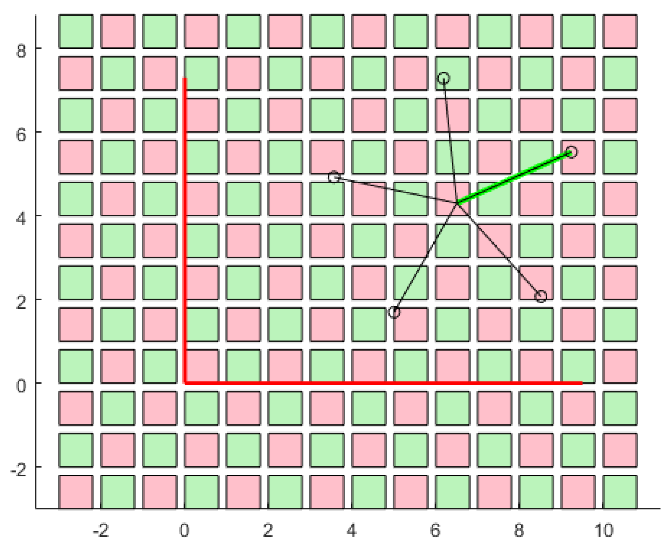
To show how the localization algorithm works we consider a particular case as an example. Assume that the actual pose of the robot is given by . This configuration is sketched in Figure 4.
Pink squares represent pads, green squares represent ones. The green segment provides a reference on the robot to identify the pins; pin 1 is the one located at the end of the green segment. The others are ordered following a counterclockwise convention. From the figure it can be inferred that pins 1, 4, and 5 are in contact with positive pads, while pin 2 is in contact with a negative pad and pin 3 lays on the insulated area; therefore the robot is powered. The estimated pose of the robot provided by the localization algorithm is and the error bounding boxes are .
3. Prototype Implementation
In this section we describe the physical realization of the prototype that we used to validate the design and to perform the measurements.
As already mentioned, power sent to the lines is suitably modulated in order to provide each line with a specific identification code related to its position on the floor. The robot extracts the DC power using a multi-phase diode bridge connected to all its pins. It then computes the row or column position of each pin by analyzing the voltage of the pin with respect to ground.
3.1. Power Modulation
All the rows are powered simultaneously. However a different identification code is used or each row; the same applies to columns. Rows and columns are alternatively powered, the other ones (i.e., columns or rows, respectively) being left connected to ground. The repetition period is 14 .
For implementation reasons (see below), rows are grouped in lanes, the lane number being a part of the line identification code; the same applies to columns.
The identification code is based on a simple PWM scheme: the duty cycle D is set to 33% for 0 s and 66% for 1 s, with a bit period of , and the code is built as follows:
- a long ( ) start pulse is used to ease synchronization at the receiver;
- 3 bits are used to identify the lane; even lane numbers are used for rows, odd lane numbers for columns;
- 4 bits are used to identify the row or column within the lane;
- finally, a stop bit (always 0 in the present implementation) completes the code.
Figure 5 shows an example of the voltages on two rows and two columns.
The selection of the repetition period is a trade-off between temporal resolution and communication reliability, and takes into account the robot mechanical speed. As already mentioned, we choose a value of 14 , which means that the pose of the robot can be updated 70 times per second.
It is apparent that the present code limits the extension of the floor to a square of 64 rows and 64 columns; obviously, larger floors can be used by simply adding bits to the code.
In the case where there is a contact with at least one pad powered with and one pad powered with , it has to be noted that:
- a voltage difference is available both when and when ,
- the average duty cycle of the PWM code, start pulse not included, is 50%,
- the short dead time at the end of the bursts is partially compensated by the long start pulse.
Hence, it follows that power can be extracted from the floor for approximately 50% of the time.
3.2. Powered Floor
For the development of the prototype of the floor we followed a modular approach: indeed, the floor is obtained by juxtaposition of several suitably designed identical Printed Circuit Boards (PCBs), which we call tiles. This allows us to build a rectangular floor of (virtually) any size simply by connecting a suitable number of them. Each tile is a PCB with 10 rows and 10 columns of contact pads; each pad is wide (i.e., ), the distance between the pads being (i.e., ). Each tile is connected to its 4 nearest neighbors via suitable connections located along the four sides, on the back of the circuit.
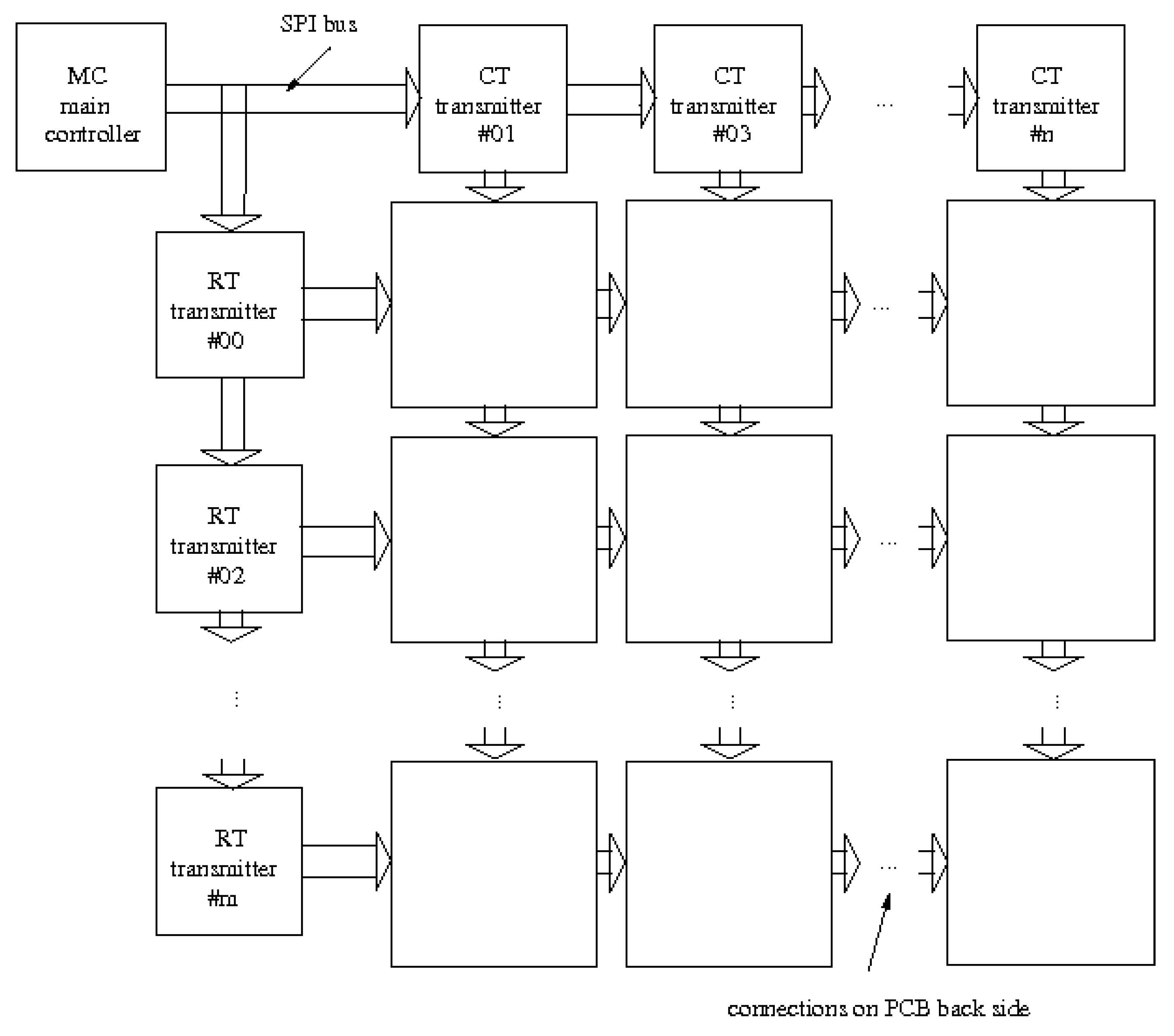
Along the upper and left border of the floor we put a set of another type of modules, called transmitters and shown in Figure 6. Each of these modules provides power and row/column identification to the first tile of a row (in case of RT, row transmitters) or column (CT, column transmitter): each tile in turn propagates power and identification to the next one both to the right and below via the already mentioned connections on the back of the PCB. Each transmitter takes care of one lane of 10 rows or 10 columns, so that we have a lane of 10 rows (or columns) for each row (or columns) of tiles. All the transmitters are controlled by another module, called main controller (MC).
In our prototype we used tiles, so that overall the floor has 20 rows and 20 columns. A picture of the prototype, together with the robot, is shown in Figure 7.
3.2.1. Main Controller
In order to manage the relatively large number of lines, we use a microcontroller (in particular, a low cost dual-core ESP32 SoC) which acts as Serial Peripheral Interface (SPI) master and controls several MCP23S17 16 bit SPI I/O expanders, one for each transmitter.
Once the topology of the floor (i.e., the number and position of tiles) is chosen, the code we define is fixed; consequently, a simple way to generate the identification codes for the power lines is to use a lookup table (LUT). At startup, the MC initializes the LUT with all the codes for the power lines; during operation, it periodically sends these codes to the RTs and CTs, which actually drive the power lines.
3.2.2. Transmitters
Each transmitter is identified by a numerical code, which is set on its PCB via jumpers; this code is even for RTs and odd for CTs and corresponds to the lane number.
As already mentioned, each transmitter is based on an MCP23S17 16 bit SPI I/O expander; it receives the commands from the MC and generates the signals for the power lines. All the transmitters are connected to the same SPI bus; the transmitter identification code is used by each transmitter to know which data it has to read from the SPI buffer.
As the transmitters must provide a relatively large current for the robot power supply, the outputs of each expander (actually, 10 of them, the remaining 6 being left unused) are buffered by three L293 drivers.
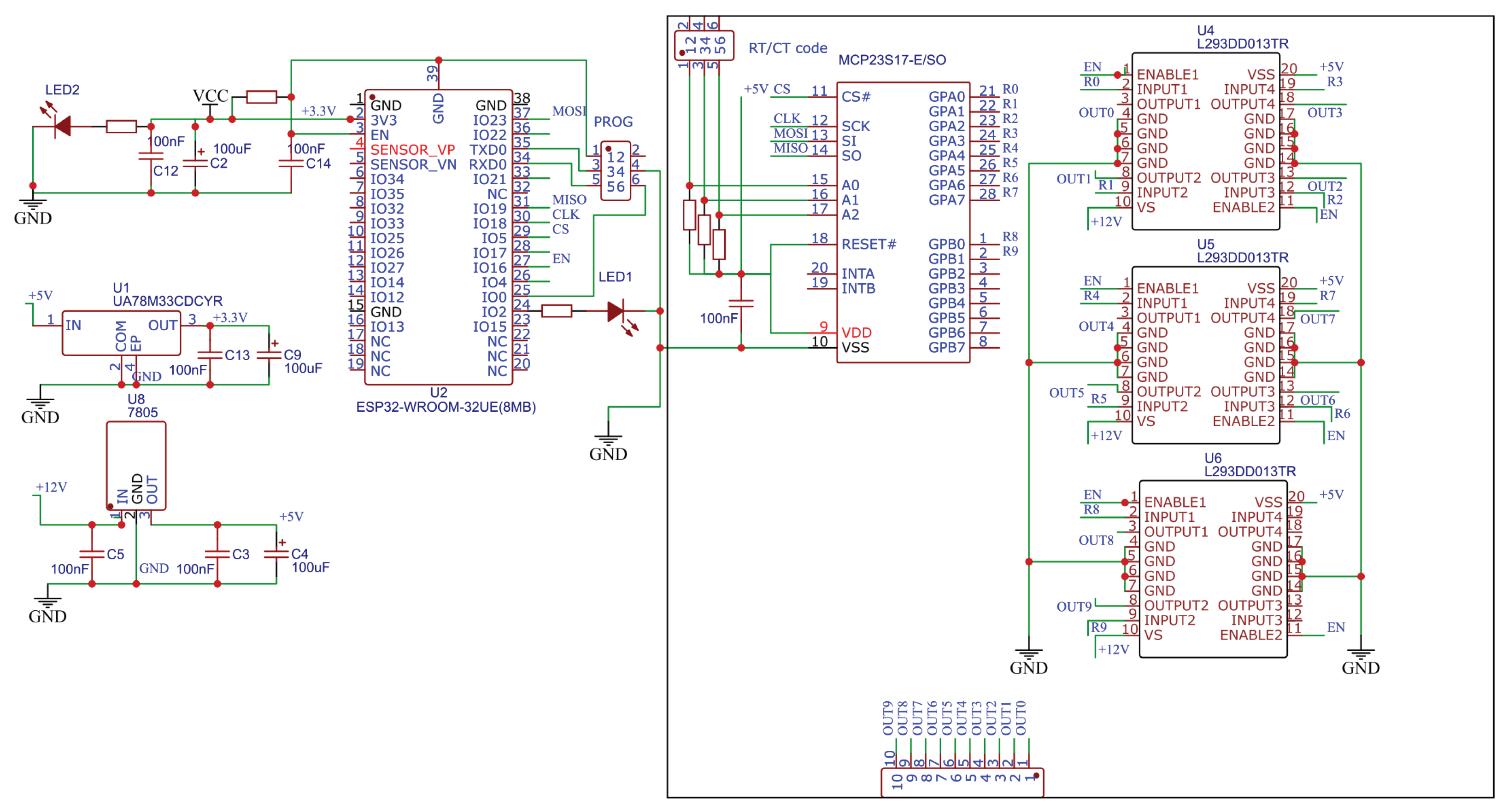
The schematic diagram of the MC and one transmitter is reported in Figure 8.
3.2.3. Tiles
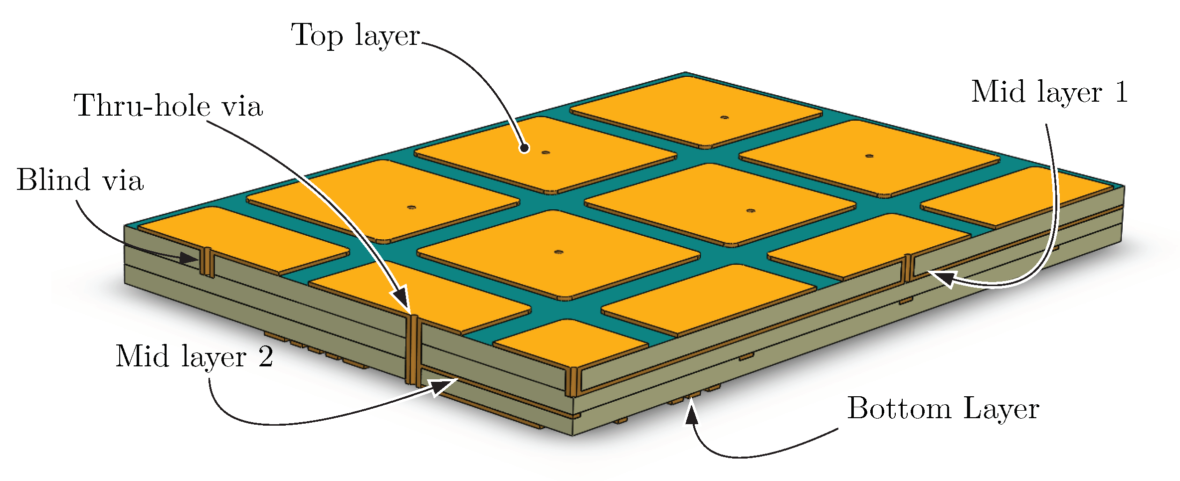
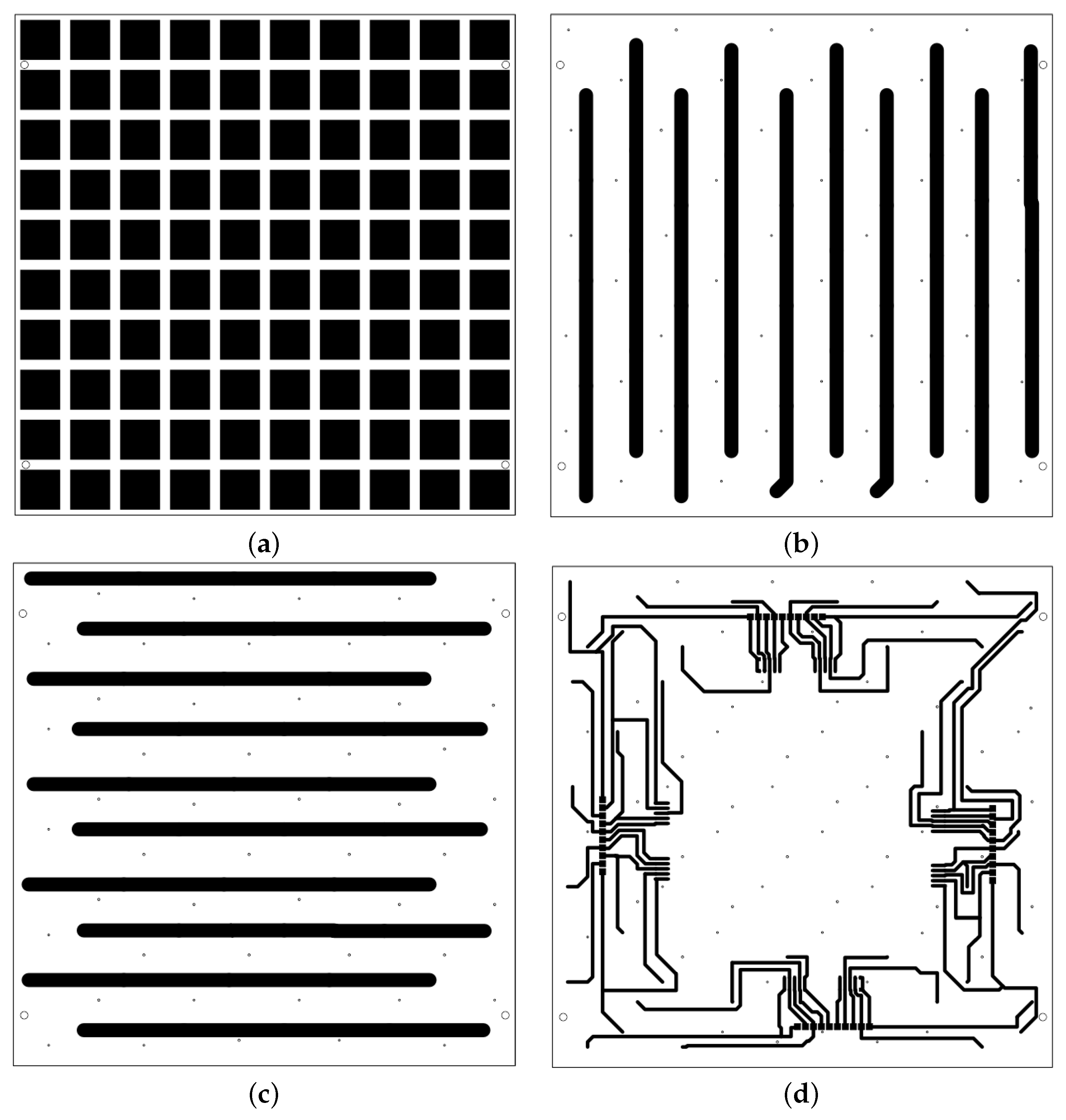
As previously mentioned, each tile is a suitably designed PCB, which takes care of both power and signal routing and exposition of the contact pads for the robot. Due to the presence of the pads, it was necessary to use a 4 layer stack-up (see Figure 9).
More in detail, with reference to Figure 10, the top layer exposes the contact pads, mid layer 1 carries the power/signal column lines, mid layer 2 carries the power/signal row lines, the bottom layer routes the column or row lines to the connectors placed along the sides of the PCB.
3.3. The Robot
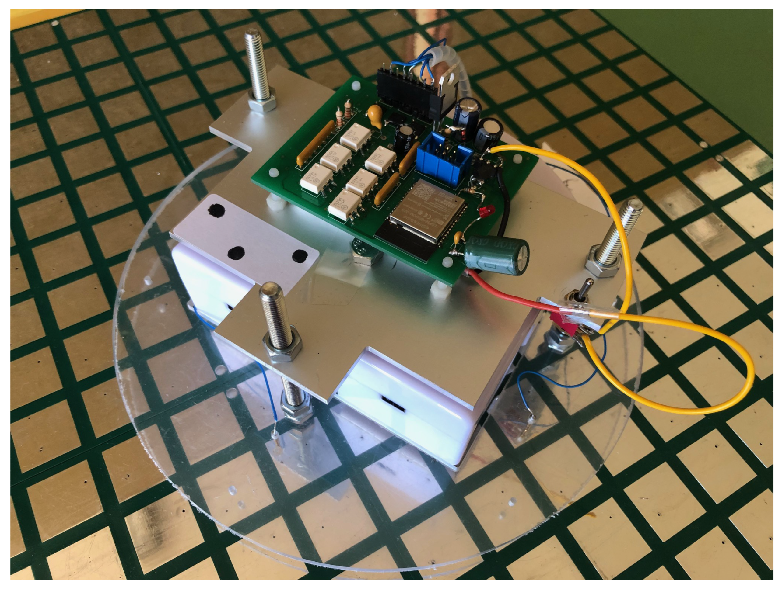
As already mentioned, we used a Thymio-II robot. It is a differential wheel robot, which we modified in order to accommodate the pins and the electronics for the power supply and the pose estimation.
As shown in Figure 7, we added a Plexiglas (PMMA, polymethyl methacrylate) disk at the base of the robot; we arranged the 5 contact pins along its circumference. Finally, we placed a white label on the top on the robot; the three black dots serve as a marker for a computer vision system, whose camera we placed above the floor. We used this setup to validate the results of our pose estimation algorithm with the experimental campaign described below.
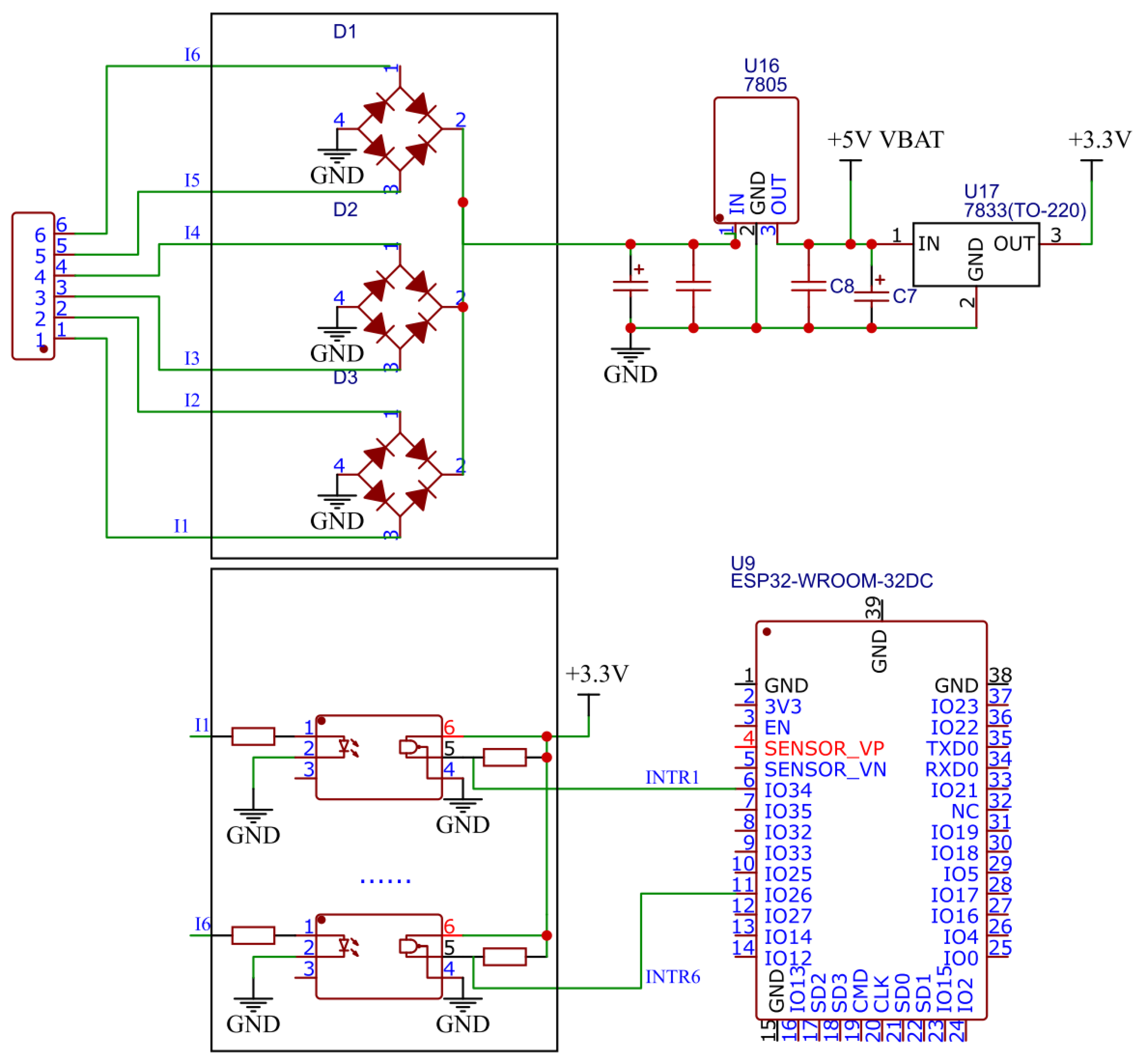
Receiver Electronics
The receiver, also based on an ESP32 SoC, extracts both power and identification signals from the waveforms coming from the input pins. DC power is obtained via a multi-phase diode bridge followed by two linear regulators, one for the battery and the other for the microcontroller.
The signals coming from each pin are photocoupled (we used H11L1 photocouplers) and sent to the microcontroller, which computes the on- and off-times of each input waveform and retrieves the corresponding identification codes using a suitable look-up table. The schematic diagram of the receiver is reported in Figure 11.
As the ESP32 provides both Bluetooth and Wi-Fi connectivity, the robot pose can be easily sent to an external PC in order to either check the system functionality during the test phase, or to analyze the robot behavior.
4. Test Results
We performed an experimental evaluation with a dual goal. On the one hand, we aimed at showing that the robot can be correctly powered; on the other hand, we wanted to validate the pose estimation provided by the localization algorithm.
In order to measure the robot pose precisely, we used a computer vision system as an external pose estimation method. We placed a camera above the powered floor, facing downwards in such a way as to evaluate, moment by moment, the pose of the robot relative to a reference frame overlayed to the edge of the floor. We calibrated the camera to eliminate optical distortions and perspective errors and fed the video stream to a video tracking software (realized in Matlab), able to determine the position of the robot with an accuracy of 2 .
During the experiments, we moved the robot along a set of planned trajectories (using the Thymio-II remote controller), we acquired the electrical signals and recorded the video stream. For each trajectory, we kept note of the position of the robot obtained by the vision system and compared it against the pose estimated by the localization module. An example of comparison of the two values can be seen in Figure 12. The red curve represents the actual trajectory of the robot; the blue line represents the trajectory computed by the localization module; the black line rectangles represent the error range along x and y coordinates as estimated by Equation (23) (i.e., the size of each rectangle is ). As it can be seen, the actual trajectory of the robot falls, for its largest part, within the envelope of all the rectangles; this shows that the localization system works correctly. By observing the relative position of the red (actual trajectory) and blue (computed trajectory) lines in Figure 12, it can be seen that the distance between the two tends to be larger when the robot crosses, while moving, tiles of the powered floor. This is when one or more pins change the stripe they are in contact with and, as a consequence, the estimated x and y change.
It may be noticed that the rectangles have different sizes. This is due to the fact that there are poses of the robot for which not all pins are in contact with the pads; in principle, the fewer the number of pins, the greater the error with which the position is estimated. Also, there are some poses of the robot that do not allow the localization. This is because if the robot is not powered it is obviously not possible to activate the localization procedure.
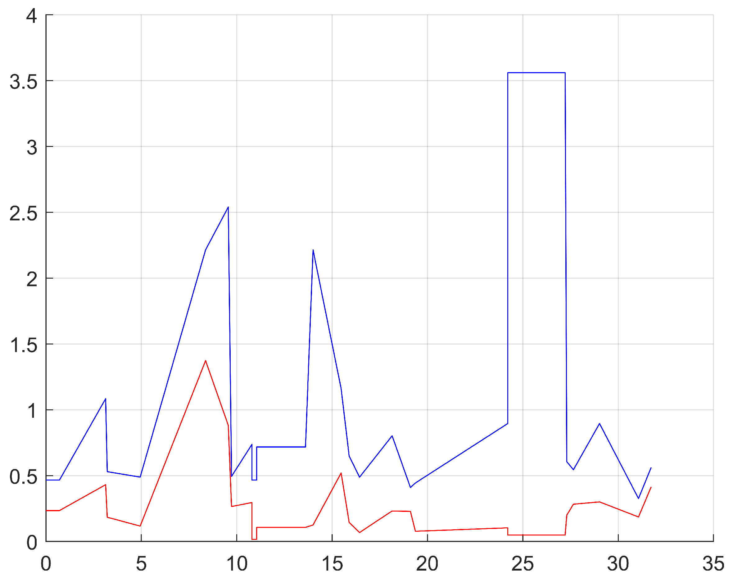
The graph in Figure 13 represents the comparison between actual errors and the estimated errors during robot advancement. Specifically, the distance traveled by the robot is represented in the abscissa; we emphasize that the distance is normalized with respect to the pitch of the square contact (). The red line represents the actual error corresponding to the difference (Euclidean distance) between the estimated position of the robot and its actual position detected by the vision system. The blue line represents a parameter related to the “estimated error window,” precisely . As it can be noticed, the measured errors are smaller than the estimated errors.
5. Conclusions
In this paper, we presented a novel power supply system for mobile robots. One relevant use-case for our system is the execution of long-lasting experiments with mobile robots (as, e.g., in swarm robotics, multi-agent systems, or evolutionary robotics) where localization is needed.
Our system consists of a floor made of conductive pads arranged in a checkerboard pattern. Each pad carries both power and digital signals, so that each robot is able to determine its pose (i.e., position and orientation).
We presented the theoretical framework describing how the geometrical design of the powered floor affects the effectiveness of power delivery and how an estimate of the robot pose can be obtained, with error boundaries. We also described in detail a prototype of the system, including the floor and the robot (obtained by modifying a commercially available robot) that we used for experimentally validating both the power delivery and the localization capabilities of our powered floor.
Author Contributions
Conceptualization, S.S., S.C., P.G.; investigation, S.S., S.C., E.M. and P.G.; methodology, E.M. and P.G.; resources, S.S.; software, A.C.; supervision, P.G.; validation, A.C. and A.Z.; writing—original draft, S.S. and P.G.; writing—review & editing, S.S. and E.M. All authors have read and agreed to the published version of the manuscript.
Funding
The work has been supported by the University of Trieste via the “University funding for scientific Research projects—FRA 2018” and by the PRIN 2017 project “SEDUCE” n. 2017TWRCNB from the Italian Ministry of University and Research.
Data Availability Statement
No new data were created or analyzed in this study; data sharing is not applicable to this article. The code used for the simulation and the experimental test, and the CAD files of the PCBs (transmitter, receiver and tiles) of the prototype are available on request from the corresponding author.
Acknowledgments
The Laboratory for Advanced Mechatronics—LAMA FVG is gratefully acknowledged for technical support. LAMA FVG is an international research center for product and process innovation where the three Universities of Friuli Venezia Giulia Region (Italy) synergically cooperate to promote R&D activities at academic and industrial level.
Conflicts of Interest
The authors declare no conflict of interest. The funders had no role in the design of the study; in the collection, analyses, or interpretation of data; in the writing of the manuscript; or in the decision to publish the results.
References
- Seriani, S.; Medvet, E.; Carrato, S.; Gallina, P. A Complete Framework for the Synthesis of Powered Floor Systems. IEEE/ASME Trans. Mechatron. 2020, 25, 1045–1055. [Google Scholar] [CrossRef] [Green Version]
- Rezvanizaniani, S.; Liu, Z.; Chen, Y.; Lee, J. Review and recent advances in battery health monitoring and prognostics technologies for electric vehicle (EV) safety and mobility. J. Power Sources 2014, 256, 110–124. [Google Scholar] [CrossRef]
- Shing, A.; Wong, P. Wear of pantograph collector strips. Proc. Inst. Mech. Eng. Part J. Rail Rapid Transit 2008, 222, 169–176. [Google Scholar] [CrossRef]
- Ding, T.; Chen, G.; Bu, J.; Zhang, W. Effect of temperature and arc discharge on friction and wear behaviours of carbon strip/copper contact wire in pantograph-catenary systems. Wear 2011, 271, 1629–1636. [Google Scholar] [CrossRef]
- Pastena, L. A Catenary-Free Electrification for Urban Transport: An Overview of the Tramwave System. IEEE Electrif. Mag. 2014, 2, 16–21. [Google Scholar] [CrossRef]
- Mei, Y.; Lu, Y.H.; Hu, Y.; Lee, C. A case study of mobile robot’s energy consumption and conservation techniques. In Proceedings of the 2005 International Conference on Advanced Robotics—ICAR ‘05, Seattle, WA, USA, 18–20 July 2005; Volume 2005, pp. 492–497. [Google Scholar]
- Sadrpour, A.; Jin, J.; Ulsoy, A. Mission energy prediction for unmanned ground vehicles using real-time measurements and prior knowledge. J. Field Robot. 2013, 30, 399–414. [Google Scholar] [CrossRef]
- Rajan, V.; Nagendran, A.; Dehghani-Sanij, A.; Richardson, R. Tether monitoring for entanglement detection, disentanglement and localisation of autonomous robots. Robotica 2016, 34, 527–548. [Google Scholar] [CrossRef] [Green Version]
- Wang, J.; Hu, M.; Cai, C.; Lin, Z.; Li, L.; Fang, Z. Optimization design of wireless charging system for autonomous robots based on magnetic resonance coupling. AIP Adv. 2018, 8, 055004. [Google Scholar] [CrossRef] [Green Version]
- Yang, M.; Yang, G.; Li, E.; Liang, Z.; Lin, H. Modeling and analysis of wireless power transmission system for inspection robot. In Proceedings of the IEEE International Symposium on Industrial Electronics, Taipei, Taiwan, 28–31 May 2013. [Google Scholar]
- Li, S.; Mi, C. Wireless power transfer for electric vehicle applications. IEEE J. Emerg. Sel. Top. Power Electron. 2015, 3, 4–17. [Google Scholar]
- Shin, J.; Shin, S.; Kim, Y.; Ahn, S.; Lee, S.; Jung, G.; Jeon, S.J.; Cho, D.H. Design and implementation of shaped magnetic-resonance-based wireless power transfer system for roadway-powered moving electric vehicles. IEEE Trans. Ind. Electron. 2014, 61, 1179–1192. [Google Scholar] [CrossRef]
- Musavi, F.; Edington, M.; Eberle, W. Wireless power transfer: A survey of EV battery charging technologies. In Proceedings of the 2012 IEEE Energy Conversion Congress and Exposition—ECCE 2012, Raleigh, NC, USA, 15–20 September 2012; pp. 1804–1810. [Google Scholar]
- Huh, J.; Lee, S.; Lee, W.; Cho, G.; Rim, C. Narrow-width inductive power transfer system for online electrical vehicles. IEEE Trans. Power Electron. 2011, 26, 3666–3679. [Google Scholar] [CrossRef]
- Marinescu, A.; Rosu, G.; Mandache, L.; Baltag, O. Achievements and Perspectives in Contactless Power Transmission. In Proceedings of the EPE 2018—2018 10th International Conference and Expositions on Electrical And Power Engineering, Iasi, Romania, 18–19 October 2018; pp. 638–645. [Google Scholar]
- Jang, Y. Survey of the operation and system study on wireless charging electric vehicle systems. Transp. Res. Part Emerg. Technol. 2018, 95, 844–866. [Google Scholar] [CrossRef]
- Hasanzadeh, S.; Vaez-Zadeh, S. A review of contactless electrical power transfer: Applications, challenges and future trends [Pregled slanja u području bezkontaktnog prijenosa električne energije: Primjene, izazovi i trendovi]. Automatika 2015, 56, 367–378. [Google Scholar] [CrossRef] [Green Version]
- Rappaport, M.; Bettstetter, C. Coordinated recharging of mobile robots during exploration. In Proceedings of the IEEE International Conference on Intelligent Robots and Systems, Vancouver, BC, Canada, 24–28 September 2017; Volume 2017, pp. 6809–6816. [Google Scholar]
- Nakamura, S.; Hashimoto, S.; Hashimoto, H. Preliminary development of an Energy Logistics as a new wireless power transmission method. In Proceedings of the IECON 2013—39th Annual Conference of the IEEE Industrial Electronics Society, Vienna, Austria, 10–13 November 2013; pp. 7843–7848. [Google Scholar]
- Seriani, S.; Gallina, P.; Wedler, A. Dynamics of a tethered rover on rough terrain. Mech. Mach. Sci. 2017, 47, 355–361. [Google Scholar]
- Seriani, S.; Gallina, P.; Wedler, A. A modular cable robot for inspection and light manipulation on celestial bodies. Acta Astronaut. 2016, 123, 145–153. [Google Scholar] [CrossRef]
- Poljanec, D.; Kalin, M.; Kumar, L. Influence of contact parameters on the tribological behaviour of various graphite/graphite sliding electrical contacts. Wear 2018, 406-407, 75–83. [Google Scholar] [CrossRef]
- Grandin, M.; Wiklund, U. Wear and electrical performance of a slip-ring system with silver-graphite in continuous sliding against PVD coated wires. Wear 2016, 348–349, 138–147. [Google Scholar] [CrossRef]
- Arvin, F.; Watson, S.; Turgut, A.; Espinosa, J.; Krajník, T.; Lennox, B. Perpetual Robot Swarm: Long-Term Autonomy of Mobile Robots Using On-the-fly Inductive Charging. J. Intell. Robot. Syst. Theory Appl. 2017, 92, 395–412. [Google Scholar] [CrossRef]
- Martel, S.; Sherwood, M.; Helm, C.; de Quevedo, W.G.; Fofonoff, T.; Dyer, R.; Bevilacqua, J.; Kaufman, J.; Roushdy, O.; Hunter, I. Three-legged wireless miniature robots for mass-scale operations at the sub-atomic scale. In Proceedings of the 2001 ICRA—IEEE International Conference on Robotics and Automation (Cat. No.01CH37164), Seoul, Republic of Korea, 21–26 May 2001; Volume 4, pp. 3423–3428. [Google Scholar]
- Seriani, S.; Scalera, L.; Gasparetto, A.; Gallina, P. A new family of magnetic adhesion based wall-climbing robots. Mech. Mach. Sci. 2019, 68, 223–230. [Google Scholar]
- Watson, R.; Ficici, S.; Pollack, J. Embodied Evolution: Distributing an evolutionary algorithm in a population of robots. Robot. Auton. Syst. 2002, 39, 1–18. [Google Scholar] [CrossRef] [Green Version]
- Klingner, J.; Kanakia, A.; Farrow, N.; Reishus, D.; Correll, N. A stick-slip omnidirectional powertrain for low-cost swarm robotics: Mechanism, calibration, and control. In Proceedings of the IEEE International Conference on Intelligent Robots and Systems, Chicago, IL, USA, 14–18 September 2014; pp. 846–851. [Google Scholar]
- Bongard, J.C. Evolutionary robotics. Commun. ACM 2013, 56, 74–83. [Google Scholar] [CrossRef] [Green Version]
- Garaffa, L.C.; Basso, M.; Konzen, A.A.; de Freitas, E.P. Reinforcement Learning for Mobile Robotics Exploration: A Survey. IEEE Trans. Neural Netw. Learn. Syst. 2021. [Google Scholar] [CrossRef] [PubMed]
- Koos, S.; Mouret, J.B.; Doncieux, S. The transferability approach: Crossing the reality gap in evolutionary robotics. IEEE Trans. Evol. Comput. 2013, 17, 122–145. [Google Scholar] [CrossRef]
- Salvato, E.; Fenu, G.; Medvet, E.; Pellegrino, F.A. Crossing the Reality Gap: A Survey on Sim-to-Real Transferability of Robot Controllers in Reinforcement Learning. IEEE Access 2021, 9, 153171–153187. [Google Scholar] [CrossRef]
- Alatise, M.B.; Hancke, G.P. Review on Challenges of Autonomous Mobile Robot and Sensor Fusion Methods. IEEE Access 2020, 8, 39830–39846. [Google Scholar] [CrossRef]
- Borenstein, J.; Everett, H.; Feng, L. Navigating Mobile Robots: Systems and Techniques; A K Peters, Ltd.: Wellesley, MA, USA, 1996. [Google Scholar]
- Magnago, V.; Corbalán, P.; Picco, G.P.; Palopoli, L.; Fontanelli, D. Robot Localization via Odometry-assisted Ultra-wideband Ranging with Stochastic Guarantees. In Proceedings of the 2019 IEEE/RSJ International Conference on Intelligent Robots and Systems (IROS), Macau, China, 4–8 November 2019; pp. 1607–1613. [Google Scholar]
- Ramezani, M.; Wang, Y.; Camurri, M.; Wisth, D.; Mattamala, M.; Fallon, M. The Newer College Dataset: Handheld LiDAR, Inertial and Vision with Ground Truth. In Proceedings of the 2020 IEEE/RSJ International Conference on Intelligent Robots and Systems (IROS), Las Vegas, NV, USA, 24 October 2020–24 January 2021; pp. 4353–4360. [Google Scholar]
- Carballido, J.; Perez-Ruiz, M.; Emmi, L.; Agüera, J. Comparison of positional accuracy between rtk and rtx gnss based on the autonomous agricultural vehicles under field conditions. Appl. Eng. Agric. 2014, 30, 361–366. [Google Scholar]
- Zmuda, M.A.; Elesev, A.; Morton, Y.T. Robot Localization Using RE and Inertial Sensor. In Proceedings of the 2008 IEEE National Aerospace and Electronics Conference, Dayton, OH, USA, 16–18 July 2008; pp. 343–348. [Google Scholar]
- Topley, M.; Richards, J.G. A comparison of currently available optoelectronic motion capture systems. J. Biomech. 2020, 106, 109820. [Google Scholar] [CrossRef] [PubMed]
- Lanzisera, S.; Lin, D.T.; Pister, K.S.J. R RF Time of Flight Ranging for Wireless Sensor Network Localization. In Proceedings of the 2006 International Workshop on Intelligent Solutions in Embedded Systems, Vienna, Austria, 30 June 2006; pp. 1–12. [Google Scholar]
- Bonin-Font, F.; Ortiz, A.; Oliver, G. Visual Navigation for Mobile Robots: A Survey. J. Intell. Robot. Syst. 2008, 53, 263–296. [Google Scholar] [CrossRef]
- Taheri, H.; Xia, Z.C. SLAM; definition and evolution. Eng. Appl. Artif. Intell. 2021, 97, 104032. [Google Scholar] [CrossRef]
Figure 1.
Schematic diagram representing the principle of interlacing the various stripes of conductors. The figure does not represent the operating procedure that was used to actually “intertwine” the conductors but only the final arrangement. The insulator bands are not represented.
Figure 1.
Schematic diagram representing the principle of interlacing the various stripes of conductors. The figure does not represent the operating procedure that was used to actually “intertwine” the conductors but only the final arrangement. The insulator bands are not represented.

Figure 2.
Positions of the 5 robot pins with respect to the conducting pads, in the inertial (a) and in the robot (b) reference frame.
Figure 2.
Positions of the 5 robot pins with respect to the conducting pads, in the inertial (a) and in the robot (b) reference frame.

Figure 3.
vs. the relative radius for different values of the number n of pins. is the sum of the widths of the conductive band and the insulator (the border of each square of the checkerboard).
Figure 3.
vs. the relative radius for different values of the number n of pins. is the sum of the widths of the conductive band and the insulator (the border of each square of the checkerboard).

Figure 4.
Example of robot pose with respect to the powered floor. The red lines are the axes of the inertial reference frame, the green segment indicates the position of the first contact pin.
Figure 4.
Example of robot pose with respect to the powered floor. The red lines are the axes of the inertial reference frame, the green segment indicates the position of the first contact pin.

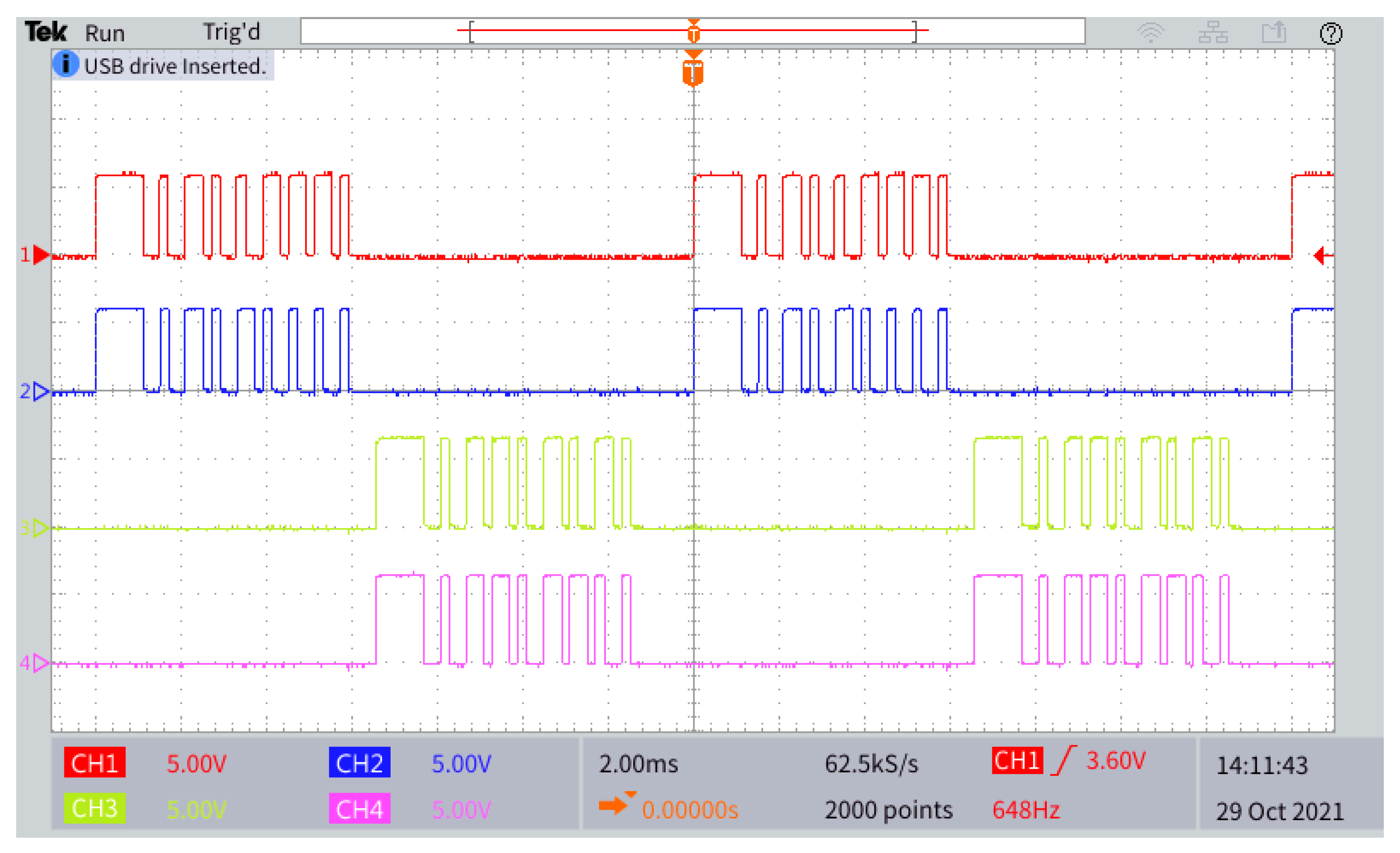
Figure 5.
Example of waveforms of and on two adjacent rows (top) and two adjacent columns (bottom), respectively. Voltages are either 0 or ; thanks to a multi-phase bridge, the robot is able to extract the to power itself. The first long pulse of each burst is the start signal: the last pulse is the stop bit, always 0. The code shown by the red trace is 01001110b: this means lane (even, this means that it is a row), line (row, in this case) , stop bit 0; similarly, for the blue trace the code is 01010000b, i.e., lane , row , stop bit 0. Similarly, the code shown by the green trace is 01101010b: this means lane (odd, this means that it is a column), line (column, in this case) , stop bit 0; similarly, for the pink trace the code is 01101100b, i.e., lane , column , stop bit 0.

Figure 6.
Block diagram of the proposed system. The white squares represent the tiles. The Main controller controls via SPI the RT and CT modules, which generate and buffer the suitable signals for the row and column lines of the tiles. These signals are propagated along the tiles, horizontally and vertically, using suitable connections placed on the back of each tile.

Figure 7.
Picture of the mobile robot positioned on the power floor. At the basis of the robot a Plexiglas disk can be seen; the 5 contact pins are positioned along its circumference. On top of the robot, the power supply and localization electronics can be seen. A white label with three black dots serves as a marker for the robot’s pose measurement system—we employed a computer vision system, placed above the floor, to validate the results of the experimental tests.

Figure 8.
Schematic diagram of the main controller (on the left) and its connection to one of the transmitters (within the rectangle).
Figure 8.
Schematic diagram of the main controller (on the left) and its connection to one of the transmitters (within the rectangle).

Figure 9.
Typical 4 layer stack-up, used for the PCB of the tiles. The bluish part represents the (isolating) protective coating over the PCB substrate (typically, FR4), while the yellow squares are the gold-plated contacts.
Figure 9.
Typical 4 layer stack-up, used for the PCB of the tiles. The bluish part represents the (isolating) protective coating over the PCB substrate (typically, FR4), while the yellow squares are the gold-plated contacts.

Figure 10.
In this figure, the conductive layers of the PCB of a tile are shown: (a) Top layer, with the gold coated square contacts, (b) Mid layer 1, for the distribution of the power supply to the contacts for which the sum of l and m (see Section 2.1) is an even number, (c) Mid layer 2, for the distribution of the power supply to the contacts for which the sum of l and m is an odd number, (d) Bottom layer, with the connections between the PCB back side connectors (see Section 3.2).

Figure 11.
Schematic diagram of the Receiver. The upper part shows the multi-phase bridge followed by two linear regulators, and is used to provide power to the robot; in the lower part, the signals coming from the contact pins (2 out of 6 are shown in the figure) are photocoupled and passed to the receiver microcontroller, which acquires them in order to compute the robot pose.

Figure 12.
Example of test of the position estimation. The red curve represents the actual trajectory of the robot obtained by the vision system. The blue curve represents the trajectory estimated through the robot internal localization system. The black rectangles represent the accuracy along the x and y coordinates for each estimated robot pose. Horizontal and vertical axes units are normalized to the pitch of the square contacts ().

Figure 13.
Comparison between actual errors (red line) and estimated errors (blue line) during robot advancement, for the path shown in Figure 12. Both the distance covered by the robot and the errors are normalized to the pitch of the square contacts ().
Figure 13.
Comparison between actual errors (red line) and estimated errors (blue line) during robot advancement, for the path shown in Figure 12. Both the distance covered by the robot and the errors are normalized to the pitch of the square contacts ().


Table 1.
Summary of the main robot localization techniques.
| Technique | Context | Dimension | Requires External Sensors | Power Delivery |
|---|---|---|---|---|
| GNSS [37] | Absolute | 3D | Yes | - |
| Motion capture [39] | Absolute | 3D | Yes | - |
| RF triangulation [38,40] | Absolute | 2D/3D | - | - |
| SLAM (3D LiDAR-based) [36] | Relative | 3D | - | - |
| SLAM (Visual-based) [41] | Relative | 2D/3D | - | - |
| SLAM (2D LiDAR-based) [42] | Relative | 2D | - | - |
| Odometry [35] | Relative | 2D | - | - |
| Powered floor with localization | Absolute | 2D | Yes | Yes |
Disclaimer/Publisher’s Note: The statements, opinions and data contained in all publications are solely those of the individual author(s) and contributor(s) and not of MDPI and/or the editor(s). MDPI and/or the editor(s) disclaim responsibility for any injury to people or property resulting from any ideas, methods, instructions or products referred to in the content. |
© 2023 by the authors. Licensee MDPI, Basel, Switzerland. This article is an open access article distributed under the terms and conditions of the Creative Commons Attribution (CC BY) license (https://creativecommons.org/licenses/by/4.0/).
Share and Cite
MDPI and ACS Style
Seriani, S.; Carrato, S.; Medvet, E.; Cernigoi, A.; Zibai, A.; Gallina, P. A Powered Floor System with Integrated Robot Localization. Electronics 2023, 12, 234. https://doi.org/10.3390/electronics12010234
AMA Style
Seriani S, Carrato S, Medvet E, Cernigoi A, Zibai A, Gallina P. A Powered Floor System with Integrated Robot Localization. Electronics. 2023; 12(1):234. https://doi.org/10.3390/electronics12010234
Chicago/Turabian StyleSeriani, Stefano, Sergio Carrato, Eric Medvet, Andrea Cernigoi, Adriano Zibai, and Paolo Gallina. 2023. "A Powered Floor System with Integrated Robot Localization" Electronics 12, no. 1: 234. https://doi.org/10.3390/electronics12010234
Note that from the first issue of 2016, this journal uses article numbers instead of page numbers. See further details here.